$B\to X_{u}\,l\,\bar{\nu}_{l}$ decay distributions to order $\alpha_{s}$

Abstract:

An analytic result for the $O(\alpha_{s})$ corrections to the triple differential $B\to X_{u}\,l\,\bar{\nu}_{l}$ decay rate is presented, to leading order in the heavy-quark expansion. This is relevant for computing partially integrated decay distributions with arbitrary cuts on kinematic variables. Several double and single differential distributions are derived, most of which generalize known results. In particular, an analytic result for the $O(\alpha_{s})$ corrections to the hadronic invariant mass spectrum is presented. The effects of Fermi motion, which are important for the description of decay spectra close to infrared sensitive regions, are included. The behaviour of perturbation theory in the region of time-like momenta is also investigated.

1 Introduction

Inclusive semileptonic decays of $B$ mesons are of prime importance to determining the parameters $|V_{cb}|$ and $|V_{ub}|$ of the Cabibbo–Kobayashi–Maskawa matrix [1]. They also serve as probes for physics beyond the Standard Model, such as an extended Higgs sector [2] or right-handed weak couplings of the $b$ quark [3, 4]. The total decay rates for these processes can be calculated in a systematic expansion in inverse powers of $m_{b}$ [5, 6, 7, 8, 9, 10, 11]. The same formalism can also be applied to calculate differential decay distributions, provided a sufficient sampling of hadronic final states is ensured by kinematics. Close to the boundary of phase space, the heavy-quark expansion must be generalized into a twist expansion to account for the effects of the “Fermi motion” of the $b$ quark inside the $B$ meson [12, 13].

The leading contribution in the $1/m_{b}$ expansion is given by the free $b$-quark decay into partons, calculated in perturbation theory as a power series in $\alpha_{s}$. Several authors have computed radiative corrections to various semileptonic decay rates and spectra. In particular, the QCD corrections to the total inclusive $B\to X_{u}\,l\,\bar{\nu}_{l}$ decay rate have recently been computed to $O(\alpha_{s}^{2})$ [14], and the rate for $B\to X_{c}\,l\,\bar{\nu}_{l}$ is known to the same order from an extrapolation of exact results obtained at three different values of the invariant mass of the lepton–neutrino pair [15]. However, to our knowledge no results for the $O(\alpha_{s})$ corrections to the fully differential $B\to X\,l\,\bar{\nu}_{l}$ decay distribution have been published so far. (An early investigation of these corrections was performed in [16], where results are presented in complicated equations involving one-dimensional integrals.) Whereas this distribution by itself is not of direct phenomenological relevance (because it does not contain sufficient averaging over hadronic final states to be realistic), it is a necessary ingredient in the derivation of predictions for inclusive spectra with arbitrary cuts on kinematic variables.

Here we present analytic results for the fully differential decay rate and several double and single differential distributions for $B\to X_{u}\,l\,\bar{\nu}_{l}$ decays. Throughout, we work to leading order in the heavy-quark expansion, omitting corrections of order $(\Lambda/m_{b})^{2}$, which have been discussed by previous authors (see, e.g., [6, 7, 8, 9, 10, 11]). The QCD corrections are calculated including terms that do not contribute in the limit of vanishing lepton mass, so that our results allow treating the case of decays into $\tau$ leptons. Semileptonic decays into final states containing a charm quark will be discussed elsewhere. A technical complication arises from the presence of soft and collinear singularities, which do not cancel in the fully differential decay distribution. These unphysical singularities appear because the calculation of inclusive rates is performed using external states containing free quarks and gluons. By virtue of global quark–hadron duality, the inclusive partonic rates are dual to the corresponding hadronic rates if a sufficient averaging over many final states is performed. We set $m_{u}=0$ and regulate the infrared singularities by introducing a fictitious gluon mass $\lambda$. The limit $\lambda\to 0$ can be taken at the end of the calculation and leads to singular distributions at $p^{2}=0$, where $p$ is the total parton momentum. Inclusive spectra obtained by integration over a range in $p^{2}$ are infrared finite.

2 Hadronic tensor at next-to-leading order in $\alpha_{s}$

All strong-interaction dynamics relevant to inclusive semileptonic decays is encoded in the hadronic tensor

$$W_{\mu\nu}(p,v)=-\frac{1}{\pi}\,\mbox{Im}\,T_{\mu\nu}(p,v)\,,$$ (1)

where

$$T_{\mu\nu}(p,v)=-i\int\mbox{d}^{4}x\,e^{i(p-m_{b}v)\cdot x}\,\frac{\langle B(v)|\,\mbox{T}\{J_{\mu}^{\dagger}(x),J_{\nu}(0)\}\,|B(v)\rangle}{2M_{B}}$$ (2)

is the forward scattering amplitude given by the $B$-meson matrix element of the time-ordered product of two weak currents, with $J_{\mu}=\bar{u}\gamma_{\mu}(1-\gamma_{5})b$. For the calculation of QCD corrections it is convenient to choose the $b$-quark velocity $v$ (which can be taken to coincide with the velocity of the $B$ meson) and the total parton momentum $p$ as the two independent variables characterizing the hadronic tensor. The total momentum carried by the leptons is $q=m_{b}v-p$.

Because $v^{2}=1$, the two independent kinematic invariants are $v\cdot p$ and $p^{2}$. The most general Lorentz-invariant decomposition of the hadronic tensor contains five invariant functions $W_{i}(v\cdot p,p^{2})$, which we define as

$$W_{\mu\nu}(p,v) = W_{1}(v\cdot p,p^{2})\Big{(}p_{\mu}v_{\nu}+p_{\nu}v_{\mu}-g_{\mu\nu}\,v\cdot p-i\epsilon_{\mu\nu\alpha\beta}\,p^{\alpha}v^{\beta}\Big{)}-$$ (3)

$${}-W_{2}(v\cdot p,p^{2})\,g_{\mu\nu}+W_{3}(v\cdot p,p^{2})\,v_{\mu}v_{\nu}+$$

$${}+W_{4}(v\cdot p,p^{2})\,(p_{\mu}v_{\nu}+p_{\nu}v_{\mu})+W_{5}(v\cdot p,p^{2})\,p_{\mu}\,p_{\nu}\,.$$

At tree level $W_{1}=2\delta(p^{2})$ and $W_{i\neq 1}=0$. The five invariant functions $W_{i}$ suffice to calculate arbitrary semileptonic decay distributions, including the case where the mass of the charged lepton is not neglected. In general, these distributions can be written in terms of three independent kinematic variables. One common choice of such variables is the charged-lepton energy $E_{l}$, the total lepton energy $v\cdot q$ (both defined in the $B$-meson rest frame), and the invariant mass $q^{2}$ of the lepton pair. Here we choose a different set of variables, because the hadronic tensor is most conveniently calculated in terms of $v\cdot p$ and $p^{2}$. Besides, experimentally the neutrino cannot be detected, whereas the total invariant mass and energy of the hadronic final state can be reconstructed directly. In terms of the parton variables, these quantities are given by

$$s_{H}=p^{2}+2\bar{\Lambda}\,v\cdot p+\bar{\Lambda}^{2}\,,\qquad E_{H}=v\cdot p+\bar{\Lambda}\,,$$ (4)

where $\bar{\Lambda}=M_{B}-m_{b}$. Experimental cuts on the region of low hadronic invariant mass or energy have been suggested as efficient ways to discriminate the small $B\to X_{u}\,l\,\bar{\nu}_{l}$ signal against the much larger background from $B\to X_{c}\,l\,\bar{\nu}_{l}$ decays [17, 18, 19, 20, 21]. Such a discrimination is important for a reliable determination of the Cabibbo–Kobayashi–Maskawa matrix element $|V_{ub}|$.

Although our results allow to treat the more general case, for the purpose of our phenomenological discussion we will set $m_{l}=0$. We introduce the scaling variables

$$x=\frac{2E_{l}}{m_{b}}\,,\qquad\hat{p}^{2}=\frac{p^{2}}{m_{b}^{2}}\,,\qquad z=\frac{2v\cdot p}{m_{b}}\,,$$ (5)

in terms of which the triple differential decay rate is

$$\frac{\mbox{d}^{3}\Gamma}{\mbox{d}x\,\mbox{d}z\,\mbox{d}\hat{p}^{2}} = 12\Gamma_{0}\,\bigg{\{}(1+\bar{x}-z)(z-\bar{x}-\hat{p}^{2})\,\frac{m_{b}^{2}}{2}\,W_{1}+(1-z+\hat{p}^{2})\,\frac{m_{b}}{2}\,W_{2}+$$ (6)

$$\hskip 31.2982pt\mbox{}+[\bar{x}(z-\bar{x})-\hat{p}^{2}]\,\frac{m_{b}}{4}(W_{3}+2m_{b}W_{4}+m_{b}^{2}W_{5})\bigg{\}}\,,$$

where $\bar{x}=1-x$, and

$$\Gamma_{0}=\frac{G_{F}^{2}|V_{ub}|^{2}m_{b}^{5}}{192\pi^{3}}\,.$$ (7)

The phase space for these variables is

$$0\leq x\leq 1\,,\qquad\bar{x}\leq z\leq 1+\bar{x}\,,\qquad\hbox{max}(0,z-1)\leq\hat{p}^{2}\leq\bar{x}(z-\bar{x})\,.$$ (8)

For fixed values of $z$ and $\hat{p}^{2}$ the lepton energy can vary in the range $\frac{1}{2}(z-\sqrt{z^{2}-4\hat{p}^{2}})\leq\bar{x}\leq\frac{1}{2}(z+\sqrt{z^{2}-4\hat{p}^{2}})$, and since the hadronic tensor is independent of $x$ it is possible to integrate over this variable to obtain the double differential spectrum

$$\frac{1}{\Gamma_{0}}\,\frac{\mbox{d}^{2}\Gamma}{\mbox{d}z\,\mbox{d}\hat{p}^{2}} = 2\sqrt{z^{2}-4\hat{p}^{2}}\,\bigg{\{}[z(3-2z)-\hat{p}^{2}(4-3z)]\,\frac{m_{b}^{2}}{2}\,W_{1}+$$ (9)

$$\hskip 65.44142pt\mbox{}+6(1-z+\hat{p}^{2})\,\frac{m_{b}}{2}\,W_{2}+$$

$$\hskip 65.44142pt\mbox{}+(z^{2}-4\hat{p}^{2})\,\frac{m_{b}}{4}(W_{3}+2m_{b}W_{4}+m_{b}^{2}W_{5})\bigg{\}}\,,$$

where

$$0\leq z\leq 2\,,\qquad\hbox{max}(0,z-1)\leq\hat{p}^{2}\leq\frac{z^{2}}{4}\,.$$ (10)

Figure 1: One-loop diagrams contributing to the forward amplitude $T_{\mu\nu}(p,v)$.

It is worth stressing at this point that any perturbative description of inclusive decay rates must necessarily be formulated in terms of scheme-dependent parameters such as the $b$-quark mass $m_{b}$ and the related parameter $\bar{\Lambda}$. These parameters are well-defined to a given order in perturbation theory. In the context of our perturbative analysis, $m_{b}$ is to be identified with the one-loop pole mass of the $b$ quark. The concept of a pole mass becomes ambiguous, however, if one goes beyond perturbation theory, and in that sense neither $m_{b}$ nor $\bar{\Lambda}$ are physical quantities. We will see in section 6 that, for normalized inclusive decay spectra, all reference to these parameters disappears once the leading nonperturbative corrections are included in the heavy-quark expansion.

The $O(\alpha_{s})$ corrections to the hadronic tensor are obtained by evaluating the contributions of all physical cuts of the diagrams shown in figure 1, supplemented by wave-function renormalization graphs for the external $b$ quarks. The sum of all contributions is gauge independent and free of ultraviolet divergences. There are, however, infrared divergences for $p^{2}\to 0$ from soft and collinear gluons, which we regularize with a fictitious gluon mass $\lambda\equiv m_{b}\hat{\lambda}$. The limit $\hat{\lambda}\to 0$ is taken whenever possible. We expand the invariant functions in a perturbation series as (with $C_{F}=4/3$)

$$W_{i}(z,\hat{p}^{2})=W_{i}^{(0)}(z,\hat{p}^{2})+\frac{C_{F}\alpha_{s}}{4\pi}\,W_{i}^{(1)}(z,\hat{p}^{2})+O(\alpha_{s}^{2})\,,$$ (11)

where $\frac{m_{b}^{2}}{2}\,W_{1}^{(0)}=\delta(\hat{p}^{2})$, and all other functions vanish at leading order. Our results for the next-to-leading coefficients can be presented as follows:

$$\frac{m_{b}^{2}}{2}\,W_{1}^{(1)} = -\delta(\hat{p}^{2})\left[4\ln^{2}\!z-6\ln z+\frac{2\ln z}{1-z}+4L_{2}(1-z)+\pi^{2}+\frac{15}{2}\right]-$$

$${}-f_{\rm IR}(\hat{\lambda}^{2},z,\hat{p}^{2})+\frac{4}{\hat{p}^{2}}\left[\frac{1}{t}\ln\frac{1+t}{1-t}+\ln\frac{\hat{p}^{2}}{z^{2}}\right]+$$

$${}+1-\frac{(8-z)(2-z)}{z^{2}t^{2}}+\left[\frac{2-z}{2z}+\frac{(8-z)(2-z)}{2z^{2}t^{2}}\right]\frac{1}{t}\ln\frac{1+t}{1-t}\,,$$

$$\frac{m_{b}}{2}\,W_{2}^{(1)} = \frac{8-z}{4}+\frac{32-8z+z^{2}}{4zt^{2}}-\left[\frac{zt^{2}}{8}+\frac{4-z}{4}+\frac{32-8z+z^{2}}{8zt^{2}}\right]\frac{1}{t}\ln\frac{1+t}{1-t}\,,$$

$$\frac{m_{b}}{4}\,W_{3}^{(1)} = -\frac{8-3z}{8}+\frac{32+22z-3z^{2}}{4zt^{2}}-\frac{3(12-z)}{8t^{4}}+$$

$${}+\left[\frac{zt^{2}}{16}+\frac{5(4-z)}{16}-\frac{64+56z-7z^{2}}{16zt^{2}}+\frac{3(12-z)}{16t^{4}}\right]\frac{1}{t}\ln\frac{1+t}{1-t}\,,$$

$$\frac{m_{b}^{2}}{2}\,W_{4}^{(1)} = \frac{2}{1-z}\left[\frac{z\ln z}{1-z}+1\right]\delta(\hat{p}^{2})-1-\frac{32-5z}{2zt^{2}}+\frac{3(12-z)}{2zt^{4}}-$$

$${}-\left[\frac{8-3z}{4z}-\frac{22-3z}{2zt^{2}}+\frac{3(12-z)}{4zt^{4}}\right]\frac{1}{t}\ln\frac{1+t}{1-t}\,,$$

$$\frac{m_{b}^{3}}{4}\,W_{5}^{(1)} = \frac{2}{1-z}\left[\frac{1-2z}{1-z}\ln z-1\right]\delta(\hat{p}^{2})-\frac{8+z}{2z^{2}t^{2}}-\frac{3(12-z)}{2z^{2}t^{4}}+$$ (12)

$${}+\left[\frac{1}{4z}-\frac{2-z}{2z^{2}t^{2}}+\frac{3(12-z)}{4z^{2}t^{4}}\right]\frac{1}{t}\ln\frac{1+t}{1-t}\,.$$

Here $t=\sqrt{1-4\hat{p}^{2}/z^{2}}$, $L_{2}(x)$ is the dilogarithm, and we have omitted the step function $\theta(\hat{p}^{2})$ multiplying all regular terms. The expressions given above are regular for $t\to 0$, corresponding to the kinematic limit where $\hat{p}^{2}\to{z^{2}}/{4}$, i.e. $|\vec{p}\,|=0$.

The function $f_{\rm IR}(\hat{\lambda}^{2},z,\hat{p}^{2})$ entering the expression for $W_{1}^{(1)}$ contains all reference to the infrared regulator. It is given by

$$f_{\rm IR}(\hat{\lambda}^{2},z,\hat{p}^{2}) = \delta(\hat{p}^{2})\left[\ln^{2}\!\hat{\lambda}^{2}+(5-4\ln z)\ln\hat{\lambda}^{2}\right]+\theta(\hat{p}^{2}-\hat{\lambda}^{2})\,\frac{4(\hat{p}^{2}-\hat{\lambda}^{2})}{(\hat{p}^{2}-\hat{\lambda}^{2})^{2}+z^{2}\hat{\lambda}^{2}}+$$ (13)

$${}+\frac{\theta(\hat{p}^{2}-\hat{\lambda}^{2})}{\hat{p}^{2}}\left[\left(1-\frac{\hat{\lambda}^{2}}{\hat{p}^{2}}\right)\left(3+\frac{\hat{\lambda}^{2}}{\hat{p}^{2}}\right)+4\ln\left(\frac{\hat{\lambda}^{2}}{\hat{p}^{2}}+\frac{\hat{p}^{2}}{z^{2}}\right)\right]\,.$$

In deriving this expression we have kept the regulator in all terms that diverge stronger than a logarithm in the limit where $\hat{p}^{2}\to 0$. The terms proportional to $\delta(\hat{p}^{2})$ come from virtual corrections to the leading-order diagram, whereas the remaining terms arise from cut diagrams with the emission of a real gluon. The limit $\hat{\lambda}\to 0$ can be taken either if $\hat{p}^{2}>0$ by virtue of some experimental cut, or if the decay distribution is integrated over some range in $\hat{p}^{2}$. Studying the integrals of the function $f_{\rm IR}$ with arbitrary regular test functions $F(\hat{p}^{2})$, we find that in the sense of distributions one can replace $f_{\rm IR}(\hat{\lambda}^{2},z,\hat{p}^{2})$ by

$$f_{\rm IR}(0,z,\hat{p}^{2})=\delta(\hat{p}^{2})\left(4\ln^{2}\!z-4\ln z+\frac{\pi^{2}}{3}-\frac{5}{2}\right)+4\left(\frac{\ln\hat{p}^{2}}{\hat{p}^{2}}\right)_{\!*}-(8\ln z-7)\left(\frac{1}{\hat{p}^{2}}\right)_{\!*}\,,\qquad$$ (14)

where the $*$ distributions are defined as

$$\left(\frac{1}{\hat{p}^{2}}\right)_{\!*} = \lim_{\epsilon\to 0}\left[\frac{\theta(\hat{p}^{2}-\epsilon)}{\hat{p}^{2}}+\delta(\hat{p}^{2})\ln\epsilon\right]\,,$$

$$\left(\frac{\ln\hat{p}^{2}}{\hat{p}^{2}}\right)_{\!*} = \lim_{\epsilon\to 0}\left[\frac{\theta(\hat{p}^{2}-\epsilon)}{\hat{p}^{2}}\ln\hat{p}^{2}+\frac{1}{2}\,\delta(\hat{p}^{2})\ln^{2}\!\epsilon\right]\,.$$ (15)

This definition is such that

$$\int_{0}^{\hat{m}^{2}}\!\mbox{d}\hat{p}^{2}\,F(\hat{p}^{2})\left(\frac{1}{\hat{p}^{2}}\right)_{\!*}=F(0)\ln\hat{m}^{2}+\int_{0}^{\hat{m}^{2}}\!\mbox{d}\hat{p}^{2}\,\frac{F(\hat{p}^{2})-F(0)}{\hat{p}^{2}}\,,$$ (16)

and similarly for the second distribution, so that the $*$ can be omitted if the distributions are multiplied by a test function of $O(\hat{p}^{2})$.

Using the result (14), the $O(\alpha_{s})$ corrections to $W_{1}$ can be rewritten as

$$\frac{m_{b}^{2}}{2}\,W_{1}^{(1)} = -\delta(\hat{p}^{2})\left[8\ln^{2}\!z-10\ln z+\frac{2\ln z}{1-z}+4L_{2}(1-z)+\frac{4\pi^{2}}{3}+5\right]-$$ (17)

$$\mbox{}-4\left(\frac{\ln\hat{p}^{2}}{\hat{p}^{2}}\right)_{\!*}+(8\ln z-7)\left(\frac{1}{\hat{p}^{2}}\right)_{\!*}+\frac{4}{\hat{p}^{2}}\left[\frac{1}{t}\ln\frac{1+t}{1-t}+\ln\frac{\hat{p}^{2}}{z^{2}}\right]+$$

$$\mbox{}+1-\frac{(8-z)(2-z)}{z^{2}t^{2}}+\left[\frac{2-z}{2z}+\frac{(8-z)(2-z)}{2z^{2}t^{2}}\right]\frac{1}{t}\ln\frac{1+t}{1-t}\,.\qquad$$

The expressions (2) and (17) are the basis for all results presented in this paper.

3 Double differential distributions

The exact results for the invariant functions $W_{i}$ given above allow the calculation of arbitrary $B\to X_{u}\,l\,\bar{\nu}_{l}$ decay distributions to next-to-leading order in $\alpha_{s}$. In particular, experimental cuts on the variables $E_{l}$, $E_{H}$ and $s_{H}$ can be implemented in a straightforward way if the distributions are obtained from a numerical integration of (6). In this section, we derive analytic results for the double differential distributions in the variables $(z,\hat{p}^{2})$ and $(z,x)$ obtained after one integration of the fully differential decay distribution. These results are the basis for, e.g., the study of the hadronic energy spectrum with a cut on the charged-lepton energy (or vice versa), or the hadronic invariant mass distribution. The latter will be discussed in section 5.

3.1 Distribution in the variables $(z,\hat{p}^{2})$

Inserting the results for the invariant functions $W_{i}$ into the general relation (9), we obtain a remarkably simple expression for the double differential decay rate. Defining

$$\frac{1}{\Gamma_{0}}\,\frac{\mbox{d}^{2}\Gamma}{\mbox{d}z\,\mbox{d}\hat{p}^{2}}=2z^{2}(3-2z)\left[\delta(\hat{p}^{2})+\frac{C_{F}\alpha_{s}}{4\pi}\,E_{1}(z,\hat{p}^{2})\right]+\frac{C_{F}\alpha_{s}}{4\pi}\,E_{2}(z,\hat{p}^{2})\,,$$ (18)

where here and below we omit writing $O(\alpha_{s}^{2})$ for the neglected higher-order contributions, we find

$$E_{1}(z,\hat{p}^{2}) = -\delta(\hat{p}^{2})\left[8\ln^{2}\!z-10\ln z+\frac{2\ln z}{1-z}+4L_{2}(1-z)+5+\frac{4\pi^{2}}{3}\right]-$$

$${}-4\left(\frac{\ln\hat{p}^{2}}{\hat{p}^{2}}\right)_{\!*}+(8\ln z-7)\left(\frac{1}{\hat{p}^{2}}\right)_{\!*}+\frac{1}{\hat{p}^{2}}\left[8\ln\frac{1+t}{2}+7(1-t)\right]\,,$$

$$E_{2}(z,\hat{p}^{2}) = \frac{4z^{3}\ln z}{1-z}\,\delta(\hat{p}^{2})-4\left[2z(3-4z)-3(1-2z)\hat{p}^{2}-2\hat{p}^{4}\right]\ln\frac{1+t}{1-t}+$$ (19)

$${}+4zt\,(10-15z+8\hat{p}^{2})\,.$$

The kinematic range for the variables $z$ and $\hat{p}^{2}$ is given in (10).

3.2 Distribution in the variables $(x,z)$

Another useful distribution is obtained by integrating the triple differential decay rate over the variable $\hat{p}^{2}$ in the range specified in (8). This leaves $x$ and $z$ as kinematic variables, which allows us to compute arbitrary distributions in the charged-lepton, neutrino or hadronic energies. The result for this distribution takes a different form for the two cases $z<1$ and $z>1$. For the first case, we find

$$\left.\frac{1}{\Gamma_{0}}\,\frac{\mbox{d}^{2}\Gamma}{\mbox{d}x\,\mbox{d}z}\right|_{z<1}=12(2-x-z)(x+z-1)\left[1+\frac{C_{F}\alpha_{s}}{4\pi}\,\frac{F_{<}(x,z)}{2-x-z}\right]\,,$$ (20)

where $1-z\leq x\leq 1$, and

$$F_{<}(x,z) = -2(2-x-z)\left[\ln^{2}\!\left(\frac{x+z-1}{1-x}\right)+2L_{2}(1-z)+\frac{2\pi^{2}}{3}\right]-$$ (21)

$${}-2(5-2x-2z)\ln(1-x)-\frac{f_{1}}{15}\ln\frac{x+z-1}{1-x}+$$

$${}+\frac{zf_{2}}{15(x+z-1)}\ln\frac{z}{1-x}-\frac{f_{3}}{30}\,.$$

For the case $z>1$, we have instead

$$\left.\frac{1}{\Gamma_{0}}\,\frac{\mbox{d}^{2}\Gamma}{\mbox{d}x\,\mbox{d}z}\right|_{z>1}=\frac{C_{F}\alpha_{s}}{4\pi}\,F_{>}(x,z)\,,$$ (22)

where $0\leq x\leq 2-z$ and

$$F_{>}(x,z) = -24(2-x-z)(x+z-1)\left[\ln^{2}\!\left(\frac{x+z-1}{1-x}\right)-\ln^{2}(z-1)\right]-$$ (23)

$${}-\frac{4f_{1}}{5}\,(x+z-1)\ln(x+z-1)-\frac{4f_{4}}{5}\ln\frac{z-1}{1-x}+$$

$${}+\frac{4f_{5}}{5}\,(2-x-z)^{3}\ln(1-x)+\frac{2xf_{6}}{5}\,(2-x-z)\,.$$

In (21) and (23), the coefficients $f_{i}$ are polynomials in $x$ and $z$ given by

$$f_{1} = \left(71-44x+26x^{2}-9x^{3}+x^{4}\right)-\left(44-52x+27x^{2}-4x^{3}\right)z+$$

$${}+\left(26-27x+6x^{2}\right)z^{2}-\left(9-4x\right)z^{3}+z^{4}\,,$$

$$f_{2} = 60x-15\left(2-3x+5x^{2}\right)z+5\left(7-8x+2x^{2}\right)z^{2}-5\left(2-x\right)z^{3}+z^{4}\,,$$

$$f_{3} = 15\left(2+13x-7x^{2}+3x^{3}-x^{4}\right)+\left(37-126x-29x^{2}-32x^{3}\right)z-$$

$${}-(1-x)(17-7x)z^{2}+2(1-x)z^{3}\,,$$

$$f_{4} = \left(71-115x+40x^{2}\right)-5\left(23-4x\right)z+5\left(14-9x+15x^{2}\right)z^{2}-$$

$${}-5\left(7-8x+2x^{2}\right)z^{3}+5\left(2-x\right)z^{4}-z^{5}\,,$$

$$f_{5} = \left(1+4x-x^{2}\right)+2\left(2-x\right)z-z^{2}\,,$$

$$f_{6} = 15\left(10-6x+2x^{2}-x^{3}\right)-2\left(32+23x+16x^{2}\right)z+7\left(2-x\right)z^{2}-2z^{3}\,.\$$ (24)

In the limit $x\to 1$, we obtain the simple expression

$$\left.\frac{1}{\Gamma_{0}}\,\frac{\mbox{d}^{2}\Gamma}{\mbox{d}x\,\mbox{d}z}\right|_{x\to 1}=12z(1-z)\left[1-\frac{C_{F}\alpha_{s}}{2\pi}\,F_{1}(z,x)\right]\,,$$ (25)

where

$$F_{1}(x,z) = \ln^{2}(1-x)-2\ln z\ln(1-x)+\frac{7}{2}\ln(1-x)+$$ (26)

$${}+\ln^{2}\!z-\frac{3}{2}\ln z+\frac{\ln z}{1-z}+2L_{2}(1-z)+\frac{2\pi^{2}}{3}+\frac{5}{2}+O(1-x)\,.$$

This result, which was previously derived by Akhoury and Rothstein [22], is needed for the next-to-leading order resummation of Sudakov logarithms to all orders of perturbation theory [23, 24].

4 Single differential spectra

While the results presented in the previous section are new, there already exist several calculations of the $O(\alpha_{s})$ corrections to single differential spectra in $B\to X_{u}\,l\,\bar{\nu}_{l}$ decays. Here we derive the distributions in the variables $x$, $z$ and $\hat{p}^{2}$. This allows comparison of our results with existing calculations.

4.1 Charged-lepton energy spectrum

Integrating the double differential decay rate derived in section 3.2 over $z$ yields the spectrum in the variable $x$, which measures the energy of the charged lepton in the $B$-meson rest frame. We obtain

$$\frac{1}{\Gamma_{0}}\,\frac{\mbox{d}\Gamma}{\mbox{d}x}=2x^{2}(3-2x)\left[1-\frac{C_{F}\alpha_{s}}{2\pi}\,G(x)\right]\,,$$ (27)

where $0\leq x\leq 1$, and

$$G(x) = \ln^{2}(1-x)+2L_{2}(x)+\frac{2\pi^{2}}{3}+\frac{82-153x+86x^{2}}{12x(3-2x)}+$$ (28)

$${}+\frac{41-36x+42x^{2}-16x^{3}}{6x^{2}(3-2x)}\ln(1-x)\,.$$

This agrees with the well-known result obtained first by Jeżabek and Kühn [25].

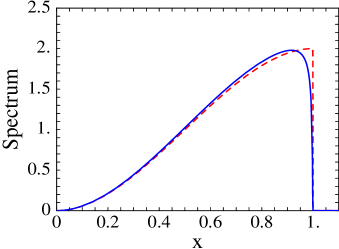
Figure 2: Lepton energy spectrum $\mbox{d}\Gamma/\mbox{d}x$ in units of $\Gamma$, at tree level (dashed) and including $O(\alpha_{s})$ corrections (solid).

The function $G(x)$ is regular for $x\!\to\!0$. On the other hand for $x\!\to\!1$, i.e. close to the boundary of phase space, there are Sudakov logarithms reflecting the incomplete cancellation of infrared divergences due to the limited phase space available for real gluon emission:

$$G(x) = \ln^{2}(1-x)+\frac{31}{6}\,\ln(1-x)+$$ (29)

$${}+\pi^{2}+\frac{5}{4}+O(1-x)\,.$$

These endpoint singularities are integrable, and the total decay rate is given by

$$\Gamma=\Gamma_{0}\left[1-\frac{C_{F}\alpha_{s}}{2\pi}\left(\pi^{2}-\frac{25}{4}\right)\right]\,.$$ (30)

In figure 2, we show the result for the charged-lepton energy spectrum obtained at leading and next-to-leading order in perturbation theory, using $\alpha_{s}=0.22$. Here and below we normalize the distributions to the total decay rate $\Gamma$, so that the spectra shown have unit area. At tree level we use $\Gamma=\Gamma_{0}$, whereas at next-to-leading order we take the result given in (30). It is evident from the figure that the perturbative corrections affect the spectral shape close to the endpoint only.

4.2 Hadronic energy spectrum

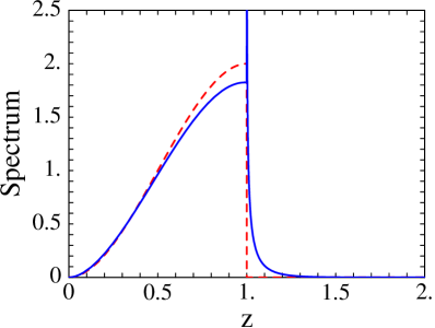
Figure 3: Hadronic energy spectrum $\mbox{d}\Gamma/\mbox{d}z$ in units of $\Gamma$, at tree level (dashed) and including $O(\alpha_{s})$ corrections (solid).

Because of the relation

$$v\cdot p = E_{H}-\bar{\Lambda}$$ (31)

$$= M_{B}-(E_{l}+E_{\bar{\nu}_{l}})-\bar{\Lambda}\,,~{}~{}$$

both the hadronic energy spectrum and the distribution of the total energy of the lepton pair can be derived from the distribution for the scaling variable $z$, which is obtained by integrating the double differential distribution in (18) over $\hat{p}^{2}$. Because of the phase-space constraintshown in (10), the resulting expressions are different for the two cases $z<1$ and $z>1$. In the second case $\hat{p}^{2}=0$ is not allowed by kinematics, and thus only diagrams with real gluon emission contribute. We find

$$\frac{1}{\Gamma_{0}}\,\frac{\mbox{d}\Gamma}{\mbox{d}z} = 2z^{2}(3-2z)\left[1-\frac{C_{F}\alpha_{s}}{2\pi}\,H_{<}(z)\right]\,,\qquad 0\leq z\leq 1\,,$$

$$\frac{1}{\Gamma_{0}}\,\frac{\mbox{d}\Gamma}{\mbox{d}z} = \frac{C_{F}\alpha_{s}}{2\pi}\,H_{>}(z)\,,\hskip 116.65646pt1\leq z\leq 2\,,$$ (32)

with

$$H_{<}(z) = 2L_{2}(1-z)+\pi^{2}+\frac{9-4z}{3-2z}\ln z-\frac{4860-3720z+585z^{2}-42z^{3}+4z^{4}}{360(3-2z)}\,,$$

$$H_{>}(z) = 2z^{2}(3-2z)\bigg{[}\ln^{2}(z-1)-2\ln^{2}\!z-4L_{2}\!\left(\frac{1}{z}\right)+\frac{\pi^{2}}{3}\bigg{]}+$$ (33)

$${}+\frac{(2-z)(1248+3798z-2946z^{2}+517z^{3}-34z^{4}+4z^{5})}{180}+$$

$${}+\frac{5+12z+12z^{2}-8z^{3}}{3}\ln(z-1)\,.$$

Our results for the functions $H_{<}(z)$ and $H_{>}(z)$ agree with the findings of Czarnecki, Jeżabek and Kühn [26]. Whereas the function $H_{<}(z)$ is regular for $z\to 1$, $H_{>}(z)$ exhibits a logarithmic divergence at this point, because the singularities from soft gluon emission are not compensated by virtual gluon corrections. We find

$$H_{>}(z)=2\ln^{2}(z-1)+7\ln(z-1)-\frac{2\pi^{2}}{3}+\frac{2587}{180}+O(z-1)\,.$$ (34)

The result for the hadronic energy spectrum at leading and next-to-leading order in perturbation theory is shown in figure 3. The double-logarithmic singularity at the point $z=1$ located inside the allowed kinematic region provides an example of a “Sudakov shoulder” [27].

4.3 Parton mass spectrum

Because the parton invariant mass $\sqrt{p^{2}}$ is not an observable quantity, the spectrum in this variable is not of direct phenomenological relevance. However, in the region $p^{2}=O(m_{b}^{2})$ it follows from (4) that $p^{2}\approx s_{H}$ up to corrections of order $\bar{\Lambda}/M_{B}$, and thus the spectrum $\mbox{d}\Gamma/\mbox{d}p^{2}$ is a reasonable approximation to the hadronic invariant mass distribution. Also, this spectrum can be used to compute moments of the hadronic mass distribution, since for instance $\langle s_{H}\rangle=m_{b}^{2}\,\langle\hat{p}^{2}\rangle+\bar{\Lambda}m_{b}\langle z\rangle+\bar{\Lambda}^{2}$. Finally, as we will discuss in section 7, the parton mass spectrum allows us to perform a quantitative study of the behaviour of perturbative QCD in the region of time-like momenta.

Integrating the double differential decay rate in (9) over $z$ in the range $2\sqrt{\hat{p}^{2}}\leq z\leq 1+\hat{p}^{2}$, we obtain

$$\frac{1}{\Gamma_{0}}\,\frac{\mbox{d}\Gamma}{\mbox{d}\hat{p}^{2}}=\delta(\hat{p}^{2})\left[1-\frac{C_{F}\alpha_{s}}{2\pi}\left(\pi^{2}+\frac{187}{72}\right)\right]+\frac{C_{F}\alpha_{s}}{2\pi}\,I(\hat{p}^{2})\,,$$ (35)

where $0\leq\hat{p}^{2}\leq 1$, and

$$I(\hat{p}^{2}) = -2\left(\frac{\ln\hat{p}^{2}}{\hat{p}^{2}}\right)_{\!*}-\frac{31}{6}\left(\frac{1}{\hat{p}^{2}}\right)_{\!*}-\left(\frac{10}{3}-6\hat{p}^{2}+\frac{4}{3}\,\hat{p}^{6}\right)\ln\hat{p}^{2}+$$ (36)

$${}+\frac{67}{9}+3\hat{p}^{2}-\frac{25}{3}\,\hat{p}^{4}+\frac{55}{18}\,\hat{p}^{6}\,.$$

The regular terms in this result, i.e. the terms that remain for $\hat{p}^{2}>0$, have been computed previously by Falk, Luke and Savage [28], and we agree with their result.

5 Hadronic invariant mass distribution

Imposing a kinematic cut $s_{H}<M_{D}^{2}$ on the inclusive semileptonic decay rate of $B$ mesons is an efficient way to separate the Cabibbo-suppressed signal from $b\to u$ transitions from the background of $b\to c$ decays [17]. Using the relation between the parton variables $p^{2}$ and $v\cdot p$ and the hadronic invariant mass displayed in (4), and denoting $\hat{s}_{H}=s_{H}/m_{b}^{2}$ and $\varepsilon=\bar{\Lambda}/m_{b}$, we find that

$$\frac{\mbox{d}\Gamma}{\mbox{d}\hat{s}_{H}}=\int_{z_{0}}^{z_{1}}\!\mbox{d}z\,\left.\frac{\mbox{d}^{2}\Gamma}{\mbox{d}z\,\mbox{d}\hat{p}^{2}}\right|_{\displaystyle\hat{p}^{2}=\hat{s}_{H}-\varepsilon z-\varepsilon^{2}}\,,\qquad\varepsilon^{2}\leq\hat{s}_{H}\leq(1+\varepsilon)^{2}\,,$$ (37)

where

$$z_{0}=2(\sqrt{\hat{s}_{H}}-\varepsilon)\,,\qquad z_{1}=\hbox{min}\!\left(\frac{\hat{s}_{H}-\varepsilon^{2}}{\varepsilon},\,1-\varepsilon+\frac{\hat{s}_{H}}{1+\varepsilon}\right)\,.$$ (38)

Because of the form of $z_{1}$, one must distinguish the cases where $\hat{s}_{H}$ is smaller or larger than $\varepsilon(1+\varepsilon)$. In the second case, only diagrams with real gluon emission contribute to the spectrum. We define

$$\frac{1}{\Gamma_{0}}\,\frac{\mbox{d}\Gamma}{\mbox{d}\hat{s}_{H}} = T(\hat{s}_{H},\varepsilon)-\frac{C_{F}\alpha_{s}}{2\pi}\,J_{<}(\hat{s}_{H},\varepsilon)\,,\qquad\varepsilon^{2}\leq\hat{s}_{H}\leq\varepsilon(1+\varepsilon)\,,$$

$$\frac{1}{\Gamma_{0}}\,\frac{\mbox{d}\Gamma}{\mbox{d}\hat{s}_{H}} = \frac{C_{F}\alpha_{s}}{2\pi}\,J_{>}(\hat{s}_{H},\varepsilon)\,,\hskip 50.07669pt\varepsilon(1+\varepsilon)\leq\hat{s}_{H}\leq(1+\varepsilon)^{2}\,.$$ (39)

The exact results for the functions entering this expression read

$$\varepsilon\,T(\hat{s}_{H},\varepsilon) = 2x^{2}(3-2x)\,,$$

$$\varepsilon\,J_{<}(\hat{s}_{H},\varepsilon) = 2x^{2}(3-2x)\left[\pi^{2}+2L_{2}(1-x)-2L_{2}\!\left(-\frac{x}{\varepsilon}\right)\right]+$$

$${}+\frac{1}{3}\,(\varepsilon d_{1}-xd_{2}-2x^{2}d_{3})(x+\varepsilon)\ln\!\left(1+\frac{x}{\varepsilon}\right)+$$

$${}+2x^{2}(9-4x)\ln x-\frac{x}{3}\bigg{(}\varepsilon d_{1}+\frac{x}{2}\,d_{4}-\frac{x^{2}}{3}\,d_{5}\bigg{)}\,,$$

$$\varepsilon\,J_{>}(\hat{s}_{H},\varepsilon) = 2x^{2}(3-2x)\times$$ (40)

$${}\times\left[\frac{\pi^{2}}{3}+\ln^{2}\!y-2\ln^{2}\!x+4L_{2}\!\left(-\frac{1}{\varepsilon}\right)-4L_{2}\!\left(\frac{1}{x}\right)-2L_{2}\!\left(-\frac{x}{\varepsilon}\right)\!\right]+$$

$${}+\frac{1}{3}\,(\varepsilon d_{1}-xd_{2}-2x^{2}d_{3})(x+\varepsilon)\ln\!\left(\frac{y+\varepsilon}{1+\varepsilon}\right)+$$

$${}+\bigg{(}7+4y-\frac{y^{2}}{\varepsilon^{2}}\,d_{6}+\frac{2y^{3}}{3\varepsilon^{3}}\,d_{7}\bigg{)}\ln y+$$

$${}+\frac{1-y}{18(1+\varepsilon)}(d_{8}+xd_{9}-2x^{2}d_{10})\,,$$

where

$$x=\frac{\hat{s}_{H}-\varepsilon^{2}}{\varepsilon}\,,\qquad y=\frac{\hat{s}_{H}-\varepsilon(1+\varepsilon)}{1+\varepsilon}\,,$$ (41)

and $d_{i}$ are polynomials in $\varepsilon$ given in equation (A) of the appendix.

Of key importance to the determination of $|V_{ub}|$ is the question which fraction of all $B\to X_{u}\,l\,\bar{\nu}_{l}$ events have hadronic invariant mass below the charm threshold. To address this issue, we compute the integral of the spectrum up to a cutoff $\hat{m}^{2}=s_{H}^{\rm max}/m_{b}^{2}$ defined as

$$\Gamma(\hat{m}^{2},\varepsilon)\equiv\int_{\varepsilon^{2}}^{\hat{m}^{2}}\!\mbox{d}\hat{s}_{H}\,\frac{\mbox{d}\Gamma}{\mbox{d}\hat{s}_{H}}\,,\qquad\varepsilon^{2}\leq\hat{m}^{2}\leq(1+\varepsilon)^{2}\,,$$ (42)

and write the result in the form

$$\Gamma(\hat{m}^{2},\varepsilon) = \Gamma_{0}\left[t(\hat{m}^{2},\varepsilon)-\frac{C_{F}\alpha_{s}}{2\pi}\,j_{<}(\hat{m}^{2},\varepsilon)\right]\,,\qquad\varepsilon^{2}\leq\hat{m}^{2}\leq\varepsilon(1+\varepsilon)\,,$$

$$\Gamma(\hat{m}^{2},\varepsilon) = \Gamma_{0}\left[1-\frac{C_{F}\alpha_{s}}{2\pi}\,j_{>}(\hat{m}^{2},\varepsilon)\right]\,,\hskip 27.03003pt\varepsilon(1+\varepsilon)\leq\hat{m}^{2}\leq(1+\varepsilon)^{2}\,.$$ (43)

Introducing the variables

$$\mu=\frac{\hat{m}^{2}-\varepsilon^{2}}{\varepsilon}\,,\qquad\varrho=\frac{\hat{m}^{2}-\varepsilon(1+\varepsilon)}{1+\varepsilon}\,,$$ (44)

we obtain

$$t(\hat{m}^{2},\varepsilon) = \mu^{3}(2-\mu)\,,$$

$$j_{<}(\hat{m}^{2},\varepsilon) = \mu^{3}(2-\mu)\left[\pi^{2}+2L_{2}(1-\mu)-2L_{2}\!\left(-\frac{\mu}{\varepsilon}\right)\right]+$$

$${}+\frac{\pi^{2}}{3}-2L_{2}(1-\mu)+\left(2\mu+\mu^{2}+\frac{20}{3}\,\mu^{3}-\frac{5}{2}\,\mu^{4}\right)\ln\mu+$$

$${}+\frac{1}{6}\left(\varepsilon^{2}e_{1}+\mu\,\varepsilon e_{2}-\mu^{2}e_{3}+\mu^{3}e_{4}\right)(\mu+\varepsilon)\ln\!\left(1+\frac{\mu}{\varepsilon}\right)-$$

$${}-\frac{\mu}{6}\,e_{5}-\frac{\mu^{2}}{12}\,e_{6}-\frac{\mu^{3}}{18}\,e_{7}+\frac{\mu^{4}}{72}\,e_{8}\,,$$

$$j_{>}(\hat{m}^{2},\varepsilon) = -\mu^{3}(2-\mu)\!\left[\frac{\pi^{2}}{3}+\ln^{2}\!\varrho-2\ln^{2}\!\mu+4L_{2}\!\left(-\frac{1}{\varepsilon}\right)-4L_{2}\!\bigg{(}\frac{1}{\mu}\bigg{)}-2L_{2}\!\left(-\frac{\mu}{\varepsilon}\right)\!\right]+$$ (45)

$${}+\pi^{2}+\ln^{2}\!\varrho-\frac{1}{6\varepsilon(1+\varepsilon)}\left(e_{9}+\mu e_{10}+\mu^{2}\varepsilon e_{11}-\mu^{3}e_{12}\right)\varrho\ln\varrho-$$

$${}-\frac{1}{6}\left(\varepsilon^{2}e_{1}+\mu\,\varepsilon e_{2}-\mu^{2}e_{3}+\mu^{3}e_{4}\right)(\mu+\varepsilon)\ln\frac{\varrho+\varepsilon}{1+\varepsilon}+$$

$${}+\frac{1}{(1+\varepsilon)^{2}}\left(\frac{1}{72}\,e_{13}-\frac{\mu}{18}\,e_{14}-\frac{\mu^{2}}{12}\,e_{15}+\frac{\mu^{3}}{18}\,e_{16}-\frac{\mu^{4}\varepsilon}{72}\,e_{17}\right)\,,$$

with coefficients $e_{i}$ given in equation (A) of the appendix.

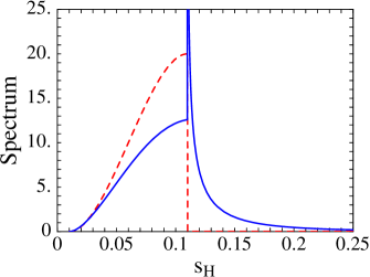
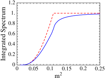
Figure 4: Left: Invariant hadronic mass spectrum $\mbox{d}\Gamma/\mbox{d}\hat{s}_{H}$ in units of $\Gamma$, at tree level (dashed) and including $O(\alpha_{s})$ corrections (solid). Right: Partially integrated spectrum $\Gamma(\hat{m}^{2},\varepsilon)$ in units of $\Gamma$.

In figure 4, we show the results for the hadronic invariant mass spectrum (left-hand plot) and for the integral of this spectrum up to a cutoff $\hat{m}^{2}$ (right-hand plot) for $\varepsilon=0.1$, corresponding to $m_{b}\approx 4.8$ GeV. Only the lower portion of the kinematic range for the variables $\hat{s}_{H}$ and $\hat{m}^{2}$ is displayed. In contrast with the energy spectra considered in the previous section, radiative corrections have an important impact on the shape of the hadronic invariant mass spectrum and lead to a significant redistribution from lower to higher masses. Nevertheless, it is apparent from the right-hand plot that imposing a cut $s_{H}<M_{D}^{2}$, corresponding to $\hat{m}^{2}\approx 0.15$, would leave most of the $B\to X_{u}\,l\,\bar{\nu}_{l}$ events unaffected but at the same time remove all $B\to X_{c}\,l\,\bar{\nu}_{l}$ events [17, 20, 21]. Because such a cut falls close to the sharp edge of the perturbative hadronic mass spectrum, however, a careful treatment of nonperturbative corrections is necessary before any conclusions can be drawn. This will be discussed in the following section.

6 Implementation of Fermi motion

The perturbative results presented above are only one ingredient to a consistent theoretical description of inclusive decay spectra. In kinematic regions close to phase-space boundaries these spectra are infrared sensitive and receive large nonperturbative corrections. Because the corresponding effects can be associated with the motion of the $b$ quark inside the $B$ meson, they are commonly referred to as “Fermi motion”. These effects are always important when the perturbative prediction for an inclusive decay distribution exhibits a rapid variation on a scale that is parametrically smaller than $m_{b}$. Usually, in such a case one encounters large perturbative corrections from Sudakov logarithms. For the single differential spectra considered in this paper, this happens in the endpoint region $1-x=O(\Lambda/m_{b})$ of the charged-lepton energy spectrum shown in figure 2, the central region $1-z=O(\Lambda/m_{b})$ of the hadronic energy spectrum shown in figure 3, and the low-mass region $\hat{s}_{H}=O(\Lambda/m_{b})$ of the hadronic invariant mass spectrum shown in figure 4. Note that in the first two cases these are small fractions of the kinematic regions; however, in the case of the hadronic mass distribution essentially all of the spectrum is concentrated in the region $\hat{s}_{H}=O(\Lambda/m_{b})$, where nonperturbative effects are important.

Fermi motion effects are included in the heavy-quark expansion by resumming an infinite set of leading-twist corrections into a shape function $F(k_{+})$, which governs the light-cone momentum distribution of the heavy quark inside the $B$ meson [12, 13]. The physical decay distributions are obtained from a convolution of parton model spectra with this function. In the process, phase-space boundaries defined by parton kinematics are transformed into the proper physical boundaries determined by hadron kinematics. The shape function is a universal characteristic of the $B$ meson governing inclusive decay spectra in processes with massless partons in the final state, such as $B\to X_{u}\,l\,\bar{\nu}_{l}$ and $B\to X_{s}\gamma$. The convolution of parton spectra with this function is such that in the perturbative formulae for the decay distributions the $b$-quark mass $m_{b}$ is replaced by the momentum dependent mass $m_{b}+k_{+}$, and similarly the parameter $\bar{\Lambda}=M_{B}-m_{b}$ is replaced by $\bar{\Lambda}-k_{+}$ [12]. Here $k_{+}$ can take values between $-m_{b}$ and $\bar{\Lambda}$, with a distribution centered around $k_{+}=0$ and with a characteristic width of $O(\Lambda)$. Introducing the new variable $q_{+}=\bar{\Lambda}-k_{+}$, it follows that, e.g., the scaling variables $x$ and $z$ are replaced by the new variables

$$x_{q}=\frac{2E_{l}}{M_{B}-q_{+}}\,,\qquad z_{q}=\frac{2(E_{H}-q_{+})}{M_{B}-q_{+}}\,,$$ (46)

and the physical spectra for the charged-lepton energy and for the total hadronic energy are, respectively, given by

$$\frac{\mbox{d}\Gamma}{\mbox{d}E_{l}}=2\!\int_{0}^{M_{B}-2E_{l}}\!\!\mbox{d}q_{+}\,\frac{F(\bar{\Lambda}-q_{+})}{M_{B}-q_{+}}\,\frac{\mbox{d}\Gamma}{\mbox{d}x}(x_{q})\,,\qquad 0\leq E_{l}\leq\frac{M_{B}}{2}\,,$$ (47)

and

$$\frac{\mbox{d}\Gamma}{\mbox{d}E_{H}}=2\int_{0}^{E_{H}}\!\mbox{d}q_{+}\,\frac{F(\bar{\Lambda}-q_{+})}{M_{B}-q_{+}}\,\frac{\mbox{d}\Gamma}{\mbox{d}z}(z_{q})\,,\qquad 0\leq E_{H}\leq M_{B}\,.$$ (48)

The perturbative spectra $\mbox{d}\Gamma/\mbox{d}x$ and $\mbox{d}\Gamma/\mbox{d}z$ have been given in (27) and (4.2). The upper limits of the $q_{+}$ integration follow from the allowed kinematic ranges for the variables $x_{q}$ and $z_{q}$. Similarly, for the hadronic invariant mass spectrum we define

$$\hat{s}_{H,q}^{2}=\frac{s_{H}}{(M_{B}-q_{+})^{2}}\,,\qquad\varepsilon_{q}=\frac{q_{+}}{M_{B}-q_{+}}\,,$$ (49)

and obtain

$$\frac{\mbox{d}\Gamma}{\mbox{d}s_{H}}=\int_{0}^{\sqrt{s_{H}}}\!\mbox{d}q_{+}\,\frac{F(\bar{\Lambda}-q_{+})}{(M_{B}-q_{+})^{2}}\,\frac{\mbox{d}\Gamma}{\mbox{d}\hat{s}_{H}}(\hat{s}_{H,q}^{2},\varepsilon_{q})\,,\qquad 0\leq s_{H}\leq M_{B}^{2}\,,$$ (50)

with $\mbox{d}\Gamma/\mbox{d}\hat{s}_{H}$ as given in (5). Here the upper limit of the $q_{+}$ integration is enforced by the requirement that $\hat{s}_{H,q}^{2}\geq\varepsilon_{q}^{2}$. From (50), it follows that the integral over the hadronic invariant mass spectrum from 0 to some cutoff $s_{H}^{\rm max}$ takes the form

$$\Gamma(s_{H}^{\rm max})\equiv\int_{0}^{s_{H}^{\rm max}}\!\mbox{d}s_{H}\,\frac{\mbox{d}\Gamma}{\mbox{d}s_{H}}=\int_{0}^{\sqrt{s_{H}^{\rm max}}}\!\mbox{d}q_{+}\,F(\bar{\Lambda}-q_{+})\,\Gamma(\hat{m}_{q}^{2},\varepsilon_{q})\,,$$ (51)

where $\hat{m}_{q}^{2}=s_{H}^{\rm max}/(M_{B}-q_{+})^{2}$, and the quantity $\Gamma(\hat{m}^{2},\varepsilon)$ has been defined in (42).

After the implementation of Fermi motion the kinematic variables take values in the entire phase space determined by hadron kinematics, rather than the parton phase space appropriate for perturbative calculations. For instance, the maximum lepton energy attainable is $E_{l}^{\rm max}=M_{B}/2$ rather than $m_{b}/2$. In the above formulae the only reference to the nonperturbative parameter $\bar{\Lambda}$ resides in the shape function. All other mass parameters refer to physical hadron masses or energies. We stress that for the numerical evaluation of the convolution integrals it is necessary to have explicit analytic results for the perturbative spectra. For the important case of the hadronic invariant mass distribution, such results have not been presented so far in the literature.

Several functional forms for the shape function have been suggested in the literature. They are subject to constraints on the moments of this function, $A_{n}=\langle k_{+}^{n}\rangle$, which are related to the forward matrix elements of local operators on the light cone [12]. The first three moments satisfy $A_{0}=1$, $A_{1}=0$ and $A_{2}=\frac{1}{3}\mu_{\pi}^{2}$, where $\mu_{\pi}^{2}$ is the average momentum squared of the $b$ quark inside the $B$ meson [29]. For our purposes, it is sufficient to adopt the simple form [30]

$$F(k_{+})=N\,(1-x)^{a}e^{(1+a)x}\,;\qquad x=\frac{k_{+}}{\bar{\Lambda}}\leq 1\,,$$ (52)

which is such that $A_{1}=0$ by construction (neglecting exponentially small terms in $m_{b}/\Lambda$), whereas the condition $A_{0}=1$ fixes the normalization $N$. The parameter $a$ can be related to the second moment, yielding $A_{2}=\frac{1}{3}\mu_{\pi}^{2}=\bar{\Lambda}^{2}/(1+a)$. Thus, the $b$-quark mass (or $\bar{\Lambda}$) and the quantity $a$ (or $\mu_{\pi}^{2}$) are the two parameters of the function. A typical choice of values is $m_{b}=4.8$ GeV and $a=1.29$, corresponding to $\bar{\Lambda}\approx 0.48$ GeV and $\mu_{\pi}^{2}\approx 0.3$ GeV². Below, we keep $a$ fixed and consider the three choices $m_{b}=4.65$, 4.8 and 4.95 GeV. The spread of the results provides a realistic estimate of the theoretical uncertainty associated with the treatment of Fermi motion. This uncertainty could be removed if the shape function were extracted, e.g., from a precise measurement of the photon energy spectrum in $B\to X_{s}\gamma$ decays [30].

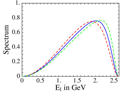
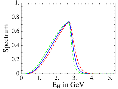
Figure 5: Left: Charged-lepton energy spectrum $\mbox{d}\Gamma/\mbox{d}E_{l}$ (in units of $\Gamma\times\mbox{GeV}^{-1}$) versus $E_{l}$ for $m_{b}=4.8$ GeV (solid), 4.65 GeV (red dashed), and 4.95 GeV (green dashed). Right: Same for the hadronic energy spectrum $\mbox{d}\Gamma/\mbox{d}E_{H}$.

Figure 5 shows the results for the charged-lepton energy spectrum and for the hadronic energy spectrum, including Fermi motion effects. The three curves in each plot correspond to different values of the $b$-quark mass. Comparing the shape of the spectra with the perturbative results shown in figures 2 and 3 indicates that for the charged-lepton energy spectrum nonperturbative effects are important in the region $E_{l}>1.8$ GeV, whereas they affect the hadronic energy spectrum in the range $2.6\,\mbox{GeV}<E_{H}<3.6$ GeV. Generally, Fermi motion effects smooth out any sharp structures in the perturbative spectra. From the results for the hadronic energy spectrum it follows that the fraction of events with $E_{H}<M_{D}$ is about $(30\pm 5)\%$, with a moderate uncertainty from the dependence on $m_{b}$. Thus, imposing a cut on the energy of the hadronic final state in $B\to X\,l\,\bar{\nu}_{l}$ decays provides a reasonably efficient way of separating the rare $b\to u$ transitions from the much larger background of $B$ decays into charmed particles [18, 19].

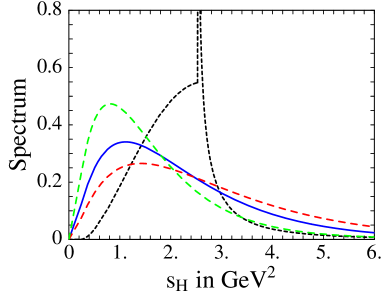
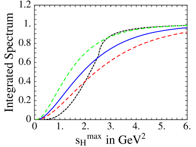
Figure 6: Left: Hadronic invariant mass spectrum $\mbox{d}\Gamma/\mbox{d}s_{H}$ (in units of $\Gamma\times\mbox{GeV}^{-2}$) versus $s_{H}$. The meaning of the curves is the same as in figure 5. In addition, the short-dashed line shows the spectrum for $m_{b}=4.8$ GeV without Fermi motion effects included. Right: Fraction of $B\to X_{u}\,l\,\bar{\nu}_{l}$ events with hadronic invariant mass below a cutoff $s_{H}^{\rm max}$.

In Figure 6, we show the results for the hadronic invariant mass spectrum and for the fraction of $B\to X_{u}\,l\,\bar{\nu}_{l}$ events with hadronic mass below a cutoff $s_{H}^{\rm max}$. In each plot, the short-dashed line shows for comparison the perturbative spectrum obtained with $m_{b}=4.8$ GeV and ignoring the effects of Fermi motion. The difference between this curve and the solid one is only due to nonperturbative effects. Clearly, these effects have a very important impact on the shape of the spectrum in the entire low-mass region relevant to experiment, and even in the region close to or above the charm threshold. Another important observation is that Fermi motion effects remove completely the sharp structure at $s_{H}\sim\bar{\Lambda}\,M_{B}$ (corresponding to $\hat{s}_{H}\sim\varepsilon(1+\varepsilon)$) in the perturbative hadronic mass spectrum and replace it by a broad bump at a significantly lower value of $s_{H}$. In other words, the value of the unphysical quantity $\bar{\Lambda}$ is of no direct relevance to the hadronic invariant mass spectrum.

From the right-hand plot in figure 6, we deduce that the fraction of events with hadronic invariant mass below the charm threshold ($s_{H}\leq 3.49$ GeV²) is about $(80\pm 10)\%$. Therefore, applying a cut $s_{H}<M_{D}^{2}$ would be a most efficient discriminator between semileptonc $b\to u$ and $b\to c$ transitions, which would allow for a largely model-independent determination of $|V_{ub}|$. If for experimental reasons the cutoff on the hadronic mass is lowered to $(1.5\,\mbox{GeV})^{2}$, the fraction of contained events drops to about $(60\pm 15)\%$, which is still significant. Even in this more pessimistic scenario, $|V_{ub}|$ could be extracted with a theoretical uncertainty of about 15%.

7 Perturbative QCD in the time-like region

As a last application, we use our results for the perturbative corrections to the inclusive $B\to X_{u}\,l\,\bar{\nu}_{l}$ decay distributions to investigate the behaviour of perturbative QCD in the region of time-like momenta. The heavy-quark expansion used in the calculation of inclusive decay rates relies on an application of the operator product expansion (OPE) in the Minkowskian region. In this region there are physical singularities from on-shell intermediate hadron states, which are not reproduced by perturbation theory. The hypothesis of quark–hadron duality is the assumption that the OPE can still be applied provided there is sufficient averaging over hadronic final states, so that the properties of individual hadron resonances become unimportant.

There is at present no known way of quantifying from first principles how well this assumption holds in the case of inclusive heavy-quark decays. In this section, we investigate the question whether perturbation theory itself signals the problem by exhibiting singularities when the resonance region is approached. To this end, we express the differential decay rate in $(z,\hat{p}^{2})$ as the imaginary part of a correlator $T(z,\hat{p}^{2})$,

$$\frac{1}{\Gamma_{0}}\,\frac{\mbox{d}^{2}\Gamma}{\mbox{d}z\,\mbox{d}\hat{p}^{2}}=\frac{1}{\pi}\,\mbox{Im}\,T(z,\hat{p}^{2}+i\epsilon)\,,$$ (53)

where $z$ is taken to be real and inside the interval $0\leq z\leq 2$. Up to irrelevant numerical factors, this correlator is the contraction of the tensor $T_{\mu\nu}(v,p)$ defined in (2) with the lepton tensor, integrated over $x$. The imaginary part is nonzero if $\hat{p}^{2}$ is in the interval given in (10). It follows that the correlator satisfies the dispersion relation

$$T(z,\hat{p}^{2})=\frac{1}{\pi}\int_{z_{0}}^{z^{2}/4}\!\mbox{d}\hat{s}\,\frac{\mbox{Im}\,T(z,\hat{s}+i\epsilon)}{\hat{s}-\hat{p}^{2}}\,,$$ (54)

where $z_{0}=\mbox{max}(0,z-1)$. In a similar way, we can express the differential spectrum in $\hat{p}^{2}$ as the imaginary part of a correlator $T(\hat{p}^{2})$,

$$\frac{1}{\Gamma_{0}}\,\frac{\mbox{d}\Gamma}{\mbox{d}\hat{p}^{2}}=\frac{1}{\pi}\,\mbox{Im}\,T(\hat{p}^{2}+i\epsilon)\,,\qquad T(\hat{p}^{2})=\frac{1}{\pi}\int_{0}^{1}\!\mbox{d}\hat{s}\,\frac{\mbox{Im}\,T(\hat{s}+i\epsilon)}{\hat{s}-\hat{p}^{2}}\,,$$ (55)

where the imaginary part is nonzero if $0\leq\hat{p}^{2}\leq 1$. With this definition, it follows that

$$T(\hat{p}^{2})=\int_{0}^{2}\!\mbox{d}z\,T(z,\hat{p}^{2})\,.$$ (56)

The correlators $T(z,\hat{p}^{2})$ and $T(\hat{p}^{2})$ as functions of complex $\hat{p}^{2}$ contain information about the behaviour of perturbation theory close to the region of physical singularities. For the purpose of illustration, we will discuss the structure of $T(\hat{p}^{2})$ in detail. An analoguous discussion could be made for the correlator $T(z,\hat{p}^{2})$ at any fixed value of $z$.

Performing the dispersion integral in (55) using the results for the $O(\alpha_{s})$ corrections given in (35) and (36), we obtain

$$T(\hat{p}^{2})=-\frac{1}{\hat{p}^{2}}\left[1-\frac{C_{F}\alpha_{s}}{2\pi}\,K(\hat{p}^{2})\right]\,,$$ (57)

where

$$K(\hat{p}^{2}) = -\left(2+\frac{10}{3}\,\hat{p}^{2}-6\hat{p}^{4}+\frac{4}{3}\,\hat{p}^{8}\right)L_{2}\bigg{(}\frac{1}{\hat{p}^{2}}\bigg{)}+$$ (58)

$${}+\left(\frac{31}{6}-\frac{41}{18}\,\hat{p}^{2}-\frac{95}{18}\,\hat{p}^{4}+\frac{55}{18}\,\hat{p}^{6}\right)(1-\hat{p}^{2})\ln\!\left(\frac{-\hat{p}^{2}}{1-\hat{p}^{2}}\right)+$$

$${}+\pi^{2}+\frac{187}{72}-6\hat{p}^{2}-\frac{233}{36}\,\hat{p}^{4}+\frac{79}{18}\,\hat{p}^{6}\,.$$

The function $K(\hat{p}^{2})$ is analytic in the cut $\hat{p}^{2}$ plane with a discontinuity along the interval $0\leq\hat{p}^{2}\leq 1$, as required by the analyticity properties of the correlator following from (55). Note that in perturbation theory the only singular point is $\hat{p}^{2}=0$, where the function has a logarithmic singularity. To get a reliable answer for a physical quantity, the region close to this singularity must be avoided.

Consider, as an example, the inclusive $B\to X_{u}\,l\,\bar{\nu}_{l}$ decay rate integrated over an interval in $\hat{p}^{2}$ including the origin:

$$\Gamma(\hat{m}^{2})\equiv\int_{0}^{\hat{m}^{2}}\!\mbox{d}\hat{p}^{2}\,\frac{\mbox{d}\Gamma}{\mbox{d}\hat{p}^{2}}=\frac{\Gamma_{0}}{2\pi i}\int_{0}^{\hat{m}^{2}}\!\mbox{d}\hat{p}^{2}\,\Big{[}T(\hat{p}^{2}+i\epsilon)-T(\hat{p}^{2}-i\epsilon)\Big{]}\,.$$ (59)

Using Cauchy’s relation, the integration contour can be deformed into a circle in the complex momentum plane touching the real axis at the point $\hat{p}^{2}=\hat{m}^{2}$. We obtain

$$\Gamma(\hat{m}^{2})=\Gamma_{0}\left[1-\frac{C_{F}\alpha_{s}}{2\pi}\int_{0}^{2\pi}\frac{\mbox{d}\varphi}{2\pi}\,K(\hat{m}^{2}e^{i\varphi})\right]\,.$$ (60)

The situation is illustrated in figure 8. Note that for $\hat{m}^{2}\geq 1$ the result of the integration is independent of $\hat{m}^{2}$, and it is thus possible to take the radius of the circle arbitrarily large, so that the contour is far away from the singularities. Therefore, is it generally accepted that the total inclusive semileptonic decay rate can be calculated reliably in perturbation theory.

Figure 7: Deformation of the integration contour in the evaluation of the quantity $\Gamma(\hat{m}^{2})$.

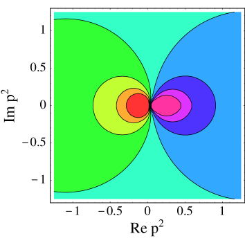
Figure 8: Contours of $\mbox{Re}\,K(\hat{p}^{2})$ in the complex $\hat{p}^{2}$ plane. The contour lines refer to values between 2.5 (innermost right contour) and 4.5 (innermost left contour) in units of 0.25.

If $\hat{m}^{2}<1$, on the other hand, the contour probes the region of physical resonances at the point where it touches the cut. It is natural to ask whether perturbation theory exhibits singularities in the vicinity of the cut, which could signal a breakdown of quark–hadron duality in the calculation of partially integrated decay rates such as $\Gamma(\hat{m}^{2})$. Remarkably, we find that this is not the case. As long as $\hat{m}^{2}$ is not too close to the origin, the perturbative corrections to the correlator $T(\hat{p}^{2})$ are well behaved everywhere in the complex momentum plane, even close to the cut. This is evident from figure 8, which shows contours of the real part of $K(\hat{p}^{2})$ in the complex $\hat{p}^{2}$ plane. We take this as an indication that partially integrated decay rates can be calculated using the heavy-quark expansion as long as they are not restricted to a range in $\hat{p}^{2}$ too close to the origin.

8 Conclusions

We have presented analytic results for the next-to-leading order perturbative corrections to the triple differential $B\to X_{u}\,l\,\bar{\nu}_{l}$ decay rate. They provide the basis for the computation of arbitrary inclusive decay distributions to $O(\alpha_{s})$, including experimental cuts on various kinematic variables. Our results are sufficiently general to allow treating the case where the mass of the charged lepton cannot be neglected. As an application, we have presented explicit results for several double and single differential distributions, most of which had not been derived previously. In particular, we have discussed in detail the $O(\alpha_{s})$ corrections to the hadronic invariant mass distribution, which are an important ingredient in a theoretically clean determination of the element $|V_{ub}|$ of the quark mixing matrix.

We have shown how the leading nonperturbative corrections affecting inclusive decay spectra can be incorporated in a QCD-based framework by convoluting the perturbative spectra with a $b$-quark momentum distribution function. This is important for addressing the question of how experimentally one may separate the $B\to X_{u}\,l\,\bar{\nu}_{l}$ signal from the large background of semileptonic decays into charmed particles. We find that $(30\pm 5)\%$ of all $B\to X_{u}\,l\,\bar{\nu}_{l}$ events have hadronic energy below the charm threshold, while $(80\pm 10)\%$ have hadronic invariant mass below $M_{D}^{2}$. If the cutoff on the hadronic mass is lowered to $(1.5\,\mbox{GeV})^{2}$, this fraction drops to $(60\pm 15)\%$, which would still allow for a largely model-independent determination of $|V_{ub}|$.

Finally, we have studied the behaviour of perturbative QCD in the complex momentum plane, finding that there is no evidence for large corrections except for the region close to $p^{2}=0$. This observation can be taken as circumstantial evidence in support of global quark–hadron duality, which underlies the heavy-quark expansion for inclusive decay rates.

Appendix A Coefficients entering the hadronic mass spectrum

Here we list the coefficients $d_{i}$ and $e_{i}$ entering the exact theoretical expressions for the hadronic invariant mass spectrum in (5), and for the integrated spectrum in (5). These coefficients are polynomials in $\varepsilon=\bar{\Lambda}/m_{b}$ given by

$$d_{1} = 9+10\varepsilon-7\varepsilon^{2}-24\varepsilon^{3}-40\varepsilon^{4}\,,$$

$$d_{2} = 9-20\varepsilon-7\varepsilon^{2}-6\varepsilon^{3}+32\varepsilon^{4}\,,$$

$$d_{3} = 1+8\varepsilon-3\varepsilon^{2}+2\varepsilon^{3}\,,$$

$$d_{4} = 153+50\varepsilon+7\varepsilon^{2}-12\varepsilon^{3}-104\varepsilon^{4}\,,$$

$$d_{5} = 167+34\varepsilon-39\varepsilon^{2}+40\varepsilon^{3}\,,$$

$$d_{6} = 3+8\varepsilon+4\varepsilon^{2}\,,$$

$$d_{7} = 1-\varepsilon-6\varepsilon^{2}-4\varepsilon^{3}\,,$$

$$d_{8} = 143+172\varepsilon+113\varepsilon^{2}+42\varepsilon^{3}-146\varepsilon^{4}-384\varepsilon^{5}-240\varepsilon^{6}\,,$$

$$d_{9} = 348+497\varepsilon+174\varepsilon^{2}-7\varepsilon^{3}-388\varepsilon^{4}-312\varepsilon^{5}\,,$$

$$d_{10} = 138+159\varepsilon-4\varepsilon^{2}+17\varepsilon^{3}+40\varepsilon^{4}\,,$$ (61)

and

$$e_{1} = 4-12\varepsilon^{2}-25\varepsilon^{3}-30\varepsilon^{4}\,,$$

$$e_{2} = 14+20\varepsilon-2\varepsilon^{2}-23\varepsilon^{3}-50\varepsilon^{4}\,,$$

$$e_{3} = 14-10\varepsilon-2\varepsilon^{2}-5\varepsilon^{3}+22\varepsilon^{4}\,,$$

$$e_{4} = 2-8\varepsilon+3\varepsilon^{2}-2\varepsilon^{3}\,,$$

$$e_{5} = 12+4\varepsilon^{2}-12\varepsilon^{4}-25\varepsilon^{5}-30\varepsilon^{6}\,,$$

$$e_{6} = 6+32\varepsilon+40\varepsilon^{2}-16\varepsilon^{3}-71\varepsilon^{4}-130\varepsilon^{5}\,,$$

$$e_{7} = 179+60\varepsilon+9\varepsilon^{2}-7\varepsilon^{3}-126\varepsilon^{4}\,,$$

$$e_{8} = 373+92\varepsilon-87\varepsilon^{2}+86\varepsilon^{3}\,,$$

$$e_{9} = 26+40\varepsilon+17\varepsilon^{2}\,,$$

$$e_{10} = 18+44\varepsilon+19\varepsilon^{2}\,,$$

$$e_{11} = 8+13\varepsilon\,,$$

$$e_{12} = 2+8\varepsilon+7\varepsilon^{2}\,,$$

$$e_{13} = 13+446\varepsilon+340\varepsilon^{2}-160\varepsilon^{3}-26\varepsilon^{4}+572\varepsilon^{5}+1428\varepsilon^{6}+1680\varepsilon^{7}+720\varepsilon^{8}\,,$$

$$e_{14} = 65+338\varepsilon+394\varepsilon^{2}+244\varepsilon^{3}-38\varepsilon^{4}-529\varepsilon^{5}-732\varepsilon^{6}-225\varepsilon^{7}+90\varepsilon^{8}\,,$$

$$e_{15} = 98+292\varepsilon+265\varepsilon^{2}+24\varepsilon^{3}-141\varepsilon^{4}-216\varepsilon^{5}+43\varepsilon^{6}+130\varepsilon^{7}\,,$$

$$e_{16} = 78+396\varepsilon+396\varepsilon^{2}+83\varepsilon^{3}+37\varepsilon^{4}-115\varepsilon^{5}-126\varepsilon^{6}\,,$$

$$e_{17} = 312+372\varepsilon+4\varepsilon^{2}+37\varepsilon^{3}+86\varepsilon^{4}\,.$$ (62)