Pion-Kaon Scattering near the Threshold in Chiral SU(2) Perturbation Theory

Abstract

In the context of chiral $SU(2)$ perturbation theory, pion-kaon scattering is analysed near the threshold to fourth chiral order. The scattering amplitude is calculated both in the relativistic framework and by using an approach similar to heavy baryon chiral perturbation theory. Both methods lead to equivalent results. We obtain relations between threshold parameters, valid to fourth chiral order, where all those combinations of low-energy constants which are not associated with chiral-symmetry breaking terms drop out. The remaining low-energy constants can be estimated using chiral $SU(3)$ symmetry. Unfortunately, the experimental information is not precise enough to test our low-energy theorems.

1 Introduction

By the end of the fifties it was clear that meson-meson scattering plays an important part in the understanding of the forces between baryons. For energies below the two-kaon threshold it is sufficient to take into account the interactions between pions. At higher energies, heavier degrees of freedom (kaon, eta, rho…) become relevant. Pion-kaon scattering – with a threshold at about $650$ MeV – constitutes the simplest mesonic system with unequal mass kinematics and carrying strangeness. For reviews of theoretical and experimental knowledge in the meson sector up to the late seventies see [1], [2], [3].

In the late seventies and early eighties, it was discovered that the low-energy structure of Green’s functions of QCD can be determined systematically [4, 5, 6]. The method – called chiral perturbation theory ($\chi{\rm PT}$) – is based on a simultaneous expansion of Green’s functions in powers of external momenta and light quark masses, the latter taking into account the breaking of the $SU(N)_{{\mbox{\tiny$R$}}}\times SU(N)_{{\mbox{\tiny$L$}}}$ (N flavour) symmetry of the strong interactions. In the context of $\chi SU(3)$ the expansion parameters $M_{\pi}^{2}/(4\pi F_{\pi})^{2}$ and $M_{{\mbox{\tiny$K$}}}^{2}/(4\pi F_{\pi})^{2}$ are of the same chiral order despite the fact that the pion mass $M_{\pi}$ is about three times smaller than the kaon mass $M_{{\mbox{\tiny$K$}}}$. Chiral $SU(3)$ perturbation theory was applied to pion-kaon scattering in [7, 8]. In these references the results for scattering lengths and other threshold parameters are given only numerically.

In 1987 $\chi{\rm PT}$ was extended to include nucleons, particles whose masses are non-zero in the chiral limit (of vanishing quark masses) [9]. Interactions of these heavy degrees of freedom with pseudo-Goldstone bosons are not constrained by the full chiral group $G=SU(2)_{{\mbox{\tiny$R$}}}\times SU(2)_{{\mbox{\tiny$L$}}}$ but only by the diagonal subgroup $H=SU(2)_{V}$. There are therefore more unknown low-energy constants than there would be in the case of ‘Goldstones’ only.

In recent years, several attempts have been made to extend the range of application of the $\chi SU(3)$ scattering amplitude to higher energies. In [10], [11] and [12] this is achieved by using unitarisation methods and dispersion relations. Another possibility of partially including higher-order corrections is to take resonances into account explicitly [13].

An S-matrix parametrisation that conforms with unitarity [14] was applied to the data of two experiments on kaon-nucleon scattering [15, 16] performed at SLAC in the seventies and eighties respectively. The authors find evidence for the existence of an $s$-wave resonance $\kappa(900)$, which constitutes an improvement in the understanding of $\pi$–$K$ partial waves. The light scalar mesons and their possible classifications are of much current interest (see for example [17]).

The purpose of the present article is to calculate the pion-kaon scattering amplitude in the context of $\chi SU(2)$ perturbation theory, where the strange quark mass is fixed by definition, to fouth chiral order and to find relations between threshold parameters where as much low-energy constants as possible cancel. An advantage of this approach is that the biggest expansion parameter (near the threshold) is now $M_{\pi}^{2}/M_{K}^{2}<M_{{\mbox{\tiny$K$}}}^{2}/(4\pi F_{\pi})^{2}$ so that the chiral expansion is expected to converge more rapidly than in the $\chi SU(3)$ theory. However, analogously to baryon $\chi{\rm PT}$, the number of low-energy constants increases.

In section 2 the chiral symmetry of the strong interactions is briefly reviewed. The role of closed kaon loops is discribed in section 3. The transformation laws of the meson fields are given in section 4 and the general effective Lagrangian is constructed in section 5. Section 6 is devoted to the chiral expansion of observables which can be extracted from the two point functions (pion and kaon masses, pion decay constant). In sections 7 and 8, we construct the isospin $3/2$ amplitude to fourth chiral order as a function of the low-energy constants. Section 9 concerns the matching of the $\chi SU(2)$ with the $\chi SU(3)$ amplitude and provides an expansion of the $\chi SU(2)$ coupling constants in powers of the strange quark mass. Low-energy theorems are given in section 10 and section 11 contains the conclusions.

2 Chiral symmetry of the strong interactions

In the limit of vanishing light-quark masses ($m_{u}=m_{d}=0$) the Lagrangian of QCD,

$${\cal L}^{\rm QCD} = -{1\over 2g^{2}}tr_{c}G_{\mu\nu}G^{\mu\nu}+{\rm i}\bar{q}_{{\mbox{\tiny$R$}}}\gamma^{\mu}(\partial_{\mu}-{\rm i}G_{\mu})q_{{\mbox{\tiny$R$}}}+{\rm i}\bar{q}_{{\mbox{\tiny$L$}}}\gamma^{\mu}(\partial_{\mu}-{\rm i}G_{\mu})q_{{\mbox{\tiny$L$}}}$$ (1)

$$\qquad-\bar{q}_{{\mbox{\tiny$R$}}}{\cal M}q_{{\mbox{\tiny$L$}}}-\bar{q}_{{\mbox{\tiny$L$}}}{\cal M}q_{{\mbox{\tiny$R$}}},$$

is invariant under global chiral transformations $(v_{{\mbox{\tiny$R$}}},v_{{\mbox{\tiny$L$}}})\in G=SU(2)_{{\mbox{\tiny$R$}}}\times SU(2)_{{\mbox{\tiny$L$}}}$. The $3\times 3$ colour matrix $G_{\mu}$ denotes the gluon field with associated field strength $G_{\mu\nu}$, and ${\cal M}={\rm diag}(m_{u},m_{d}\dots)$ is the quark-mass matrix in flavour space. The action on the chiral up- and down-quarks,

$$q_{{\mbox{\tiny$R$}}}={1\over 2}(1+\gamma_{5})q,\qquad q_{{\mbox{\tiny$L$}}}={1\over 2}(1-\gamma_{5})q,$$

is defined by

$$q_{{\mbox{\tiny$R$}}}\rightarrow v_{{\mbox{\tiny$R$}}}q_{{\mbox{\tiny$R$}}},\qquad q_{{\mbox{\tiny$L$}}}\rightarrow v_{{\mbox{\tiny$L$}}}q_{{\mbox{\tiny$L$}}}.$$

The gluon field and the heavy quarks $q_{s}$, $q_{c}$, $q_{b}$ and $q_{t}$ are not transformed under the chiral group. Therefore, these degrees of freedom are suppressed in the following. The vacuum of QCD is only assumed to be invariant under the isospin subgroup $H=SU(2)_{V}$ of $G$. According to Goldstone’s theorem [18] this implies the ocurrence of an internal $(N_{G}-N_{H})$-dimensional subspace degenerate with the vacuum, the Goldstone bosons. Here $N_{G}$ and $N_{H}$ denote the number of parameters in the Lie groups $G$ and $H$ respectively (in our case $N_{G}=6$ and $N_{H}=3$). The Green’s functions of the conserved currents as well as the scalar and pseudoscalar densities are generated by the vacuum-to-vacuum amplitude

$${\rm e}^{{\rm i}Z(r,l,s,p)}=_{\rm out}\langle\,0|0\,\rangle_{\rm in}$$

based on the Lagrangian

$${\cal L}={\cal L}^{\rm QCD}_{{\cal M}=0}+\bar{q}_{{\mbox{\tiny$R$}}}r_{\mu}\gamma^{\mu}q_{{\mbox{\tiny$R$}}}+\bar{q}_{{\mbox{\tiny$L$}}}l_{\mu}\gamma^{\mu}q_{{\mbox{\tiny$L$}}}-\bar{q}_{{\mbox{\tiny$R$}}}(s-{\rm i}p\gamma_{5})q_{{\mbox{\tiny$L$}}}-\bar{q}_{{\mbox{\tiny$L$}}}(s-{\rm i}p\gamma_{5})q_{{\mbox{\tiny$R$}}}.$$ (2)

The external fields $r_{\mu}$, $l_{\mu}$, $s$ and $p$ are hermitian colour-neutral matrices in flavour space, $r_{\mu}$ and $l_{\mu}$ being traceless. The Lagrangian (2) is now invariant under local chiral transformations provided the sources transform as

$$r_{\mu} \rightarrow v_{{\mbox{\tiny$R$}}}r_{\mu}v_{{\mbox{\tiny$R$}}}+{\rm i}v_{{\mbox{\tiny$R$}}}\partial_{\mu}v_{{\mbox{\tiny$R$}}}^{+},$$

$$l_{\mu} \rightarrow v_{{\mbox{\tiny$L$}}}l_{\mu}v_{{\mbox{\tiny$L$}}}+{\rm i}v_{{\mbox{\tiny$L$}}}\partial_{\mu}v_{{\mbox{\tiny$L$}}}^{+},$$

$$s+{\rm i}p \rightarrow v_{{\mbox{\tiny$R$}}}(s+{\rm i}p)v_{{\mbox{\tiny$L$}}}.$$

Matrix elements of vector and axial vector currents

$$V^{\mu}=\bar{q}\gamma^{\mu}\sigma^{i}q,\hskip 56.9055pt\qquad A^{\mu}=\bar{q}\gamma^{\mu}\gamma^{5}\sigma^{i}q$$

can be obtained by deriving the generating functional $Z$ with respect to

$$\begin{array}[]{cc}v_{\mu}^{i}={1\over 2}(r_{\mu}^{i}+l_{\mu}^{i})&\mbox{and }a_{\mu}^{i}={1\over 2}(r_{\mu}^{i}-l_{\mu}^{i})\end{array}$$

where $r_{\mu}^{i}$ and $l_{\mu}^{i}$ are defined by $r_{\mu}=r_{\mu}^{i}\sigma^{i}$ and $l_{\mu}=l_{\mu}^{i}\sigma^{i}$.

3 The role of closed kaon loops

The role of closed nucleon loops is analysed in the context of baryon $\chi{\rm PT}$ in [9]. The situation is analogue in the case of kaons instead of nucleons. The general effective Lagrangian describing the process $\pi K\rightarrow\pi K$ is given by a chirally symmetric string of terms

$${\cal L} = {\cal L}_{\pi\pi}+{\cal L}_{\pi K}$$

$${\cal L}_{\pi K} = {\cal L}_{KK}+{\cal L}_{KKKK}+\dots$$

The term ${\cal L}_{\pi\pi}$ does not contain the kaon field $K$ whereas ${\cal L}_{KK}$, ${\cal L}_{KKKK}$ …stand for local Lagrangians which are bilinear, quadrilinear, …in the kaon field. The bilinear term can be written in the form

$${\cal L}_{KK}=K^{+}DK$$

where $D$ denotes a $2\times 2$ matrix-differential operator which contains only the pion fields $U$ and the external sources $a_{\mu}$, $v_{\mu}$, $s$ and $p$. The explicit form of $D$ is given in section 5.1. For brevity the fields $s$, $p$ and $v_{\mu}$ are dropped in the following. With an additional source $\rho$ for the kaon field,

$$S(U,K,a,\rho)=\int{\rm d}^{4}x\left({\cal L}_{\pi\pi}+{\cal L}_{\pi K}+\rho^{+}K+K^{+}\rho\right)$$

and the vacuum transition amplitude is given by

$${}_{\rm out}\langle\,0|0\,\rangle_{\rm in} = {\rm e}^{{\rm i}Z(a,\rho,\rho^{+})}$$ (3)

$$= \int{\cal D}U{\cal D}K^{+}{\cal D}K{\rm e}^{{\rm i}S(U,K,a,\rho)}.$$

In the effective theory with pions only n-loop contributions are suppressed by a factor of $O(q^{2n})$ [4]. In the presence of heavy particles the situation is more complicated. First, there are closed kaon loops which are not suppressed. These loop contributions are real below the two-kaon threshold and, in a regularisation scheme which respects chiral symmetry, can be taken into account by a redefinition of fields and low-energy constants. This is always possible because – by construction – the general chiral Lagrangian ${\cal L}$ contains all chirally invariant structures. In particular, as we are only interested in processes with one incoming and one outgoing kaon, vertices with more than two kaon legs can be dropped. In other words, we only consider Feynman diagrams with a single uninterrupted kaon line going through the diagram. The integration over the kaon fields can therefore be performed symbolically,

$${\rm e}^{{\rm i}Z(a,\rho,\rho^{+})} = \int{\cal D}U{\cal D}K^{+}{\cal D}K{\rm e}^{{\rm i}\int{{\rm d}^{4}x\left({\cal L}_{\pi\pi}\hskip 1.42262pt+\hskip 1.42262ptK^{+}DK\hskip 1.42262pt+\hskip 1.42262pt\rho^{+}K+K^{+}\rho\right)}}$$

$$= {1\over{\rm det}(D)}\int{\cal D}U{\rm e}^{{\rm i}\int{{\rm d}^{4}x({\cal L}_{\pi\pi}\hskip 1.42262pt-\hskip 1.42262pt\rho^{+}S_{{\mbox{\tiny$K$}}}(U,a)\rho})},$$

if the low-energy constants are adjusted accordingly. Here $S_{{\mbox{\tiny$K$}}}$ denotes the kaon propagator in the presence of pion and external fields,

$$DS_{{\mbox{\tiny$K$}}}(x,y)=\delta^{4}(x-y).$$

The above argument can be used again to justify the replacement of the determinant by $1$. It’s only after this step that the low-energy constants contained in ${\cal L}_{\pi\pi}$ are rigorously the same as the ones in the original article by Gasser and Leutwyler [5].

Secondly, there are still unsuppressed loop contributions, arising from an internal kaon line, if the loop integrals are evaluated in the standard relativistic way. In the pion-nucleon case there are at least three different methods for evaluating such loop integrals in order to obtain the scattering amplitude to third chiral order. These methods, whose relationship has only been clarified recently [19, 20], will be described in section 7.

4 Effective fields and transformation laws

To model the dynamics of the pion-kaon system by an effective field theory, the action of the chiral group $G$ has to be chosen in such a way as to represent correctly the low-energy structure of QCD. The fact that the isospin subgroup leaves the vacuum invariant (in the chiral limit) means that $H$ must be the stability group (isotropy group) of each orbit of the carrier space $X$ containing the pions. This fact already implies that each orbit of $X$ must be homeomorphic to the coset space $G/H$ which is itself isomorphic to $S^{3}$ (the three-dimensional sphere) and also to $SU(2)$. It is convenient to select one representative element out of each equivalence class of $G/H$ defined by $(u_{{\mbox{\tiny$R$}}}=u,u_{{\mbox{\tiny$L$}}}=u^{+})$. This choice is unambiguous near the neutral element of $SU(2)$. The action of $(v_{{\mbox{\tiny$R$}}},v_{{\mbox{\tiny$L$}}})\in G$ on $(u_{{\mbox{\tiny$R$}}},u_{{\mbox{\tiny$L$}}})\in X$ is then:

$$(u_{{\mbox{\tiny$R$}}},u_{{\mbox{\tiny$L$}}})\rightarrow(v_{{\mbox{\tiny$R$}}}u_{{\mbox{\tiny$R$}}}h^{+},v_{{\mbox{\tiny$L$}}}u_{{\mbox{\tiny$L$}}}h^{+})$$

where the compensatory field $h\in SU(2)$ has to be chosen in such a way that $(v_{{\mbox{\tiny$R$}}}u_{{\mbox{\tiny$R$}}}h^{+},v_{{\mbox{\tiny$L$}}}u_{{\mbox{\tiny$L$}}}h^{+})$ is the representative element of the class containing $(v_{{\mbox{\tiny$R$}}}u_{{\mbox{\tiny$R$}}},v_{{\mbox{\tiny$L$}}}u_{{\mbox{\tiny$L$}}})$, i.e. so that $v_{{\mbox{\tiny$R$}}}uh^{+}=(v_{{\mbox{\tiny$L$}}}u^{+}h^{+})^{+}$. Because kaons have isospin ${1\over 2}$, this compensator can also be used to define the action of $G$ on the kaon fields $K(x)\in{\mathchoice{\hbox{\hbox to0.0pt{\kern 2.88884pt\vrule height=6.14993pt\hss}\hbox{$\displaystyle\sf C$}}}{\hbox{\hbox to0.0pt{\kern 2.88884pt\vrule height=6.14993pt\hss}\hbox{$\textstyle\sf C$}}}{\hbox{\hbox to0.0pt{\kern 2.02219pt\vrule height=4.30496pt\hss}\hbox{$\scriptstyle\sf C$}}}{\hbox{\hbox to0.0pt{\kern 1.44441pt\vrule height=3.07497pt\hss}\hbox{$\scriptscriptstyle\sf C$}}}}^{2}$:

$$\left[(u_{{\mbox{\tiny$R$}}},u_{{\mbox{\tiny$L$}}});K\right]\rightarrow\left[(v_{{\mbox{\tiny$R$}}}u_{{\mbox{\tiny$R$}}}h^{+},v_{{\mbox{\tiny$L$}}}u_{{\mbox{\tiny$L$}}}h^{+});hK\right],$$ (4)

so that in our case

$$\left(u,K\right)\rightarrow\left(v_{{\mbox{\tiny$R$}}}uh^{+},hK\right).$$ (5)

The compensator $h$ does not depend on $u$ if the action is restricted to $H$ i.e. if $v_{{\mbox{\tiny$R$}}}=v_{{\mbox{\tiny$L$}}}$. It was shown in a more general context by Coleman et al. [21] that any action on the pair $(u,K)$ respecting the chiral symmetries given above is equivalent to (5). In this work $u$ and $K$ are parameterised in terms of the physical particle fields as

$$\begin{array}[]{ll}u(x)={\rm e}^{{\rm i}{\Phi\over 2F}},&\Phi(x)=\left(\begin{array}[]{cc}\pi^{0}(x)&-\sqrt{2}\pi^{+}(x)\\ \sqrt{2}\pi^{-}(x)&-\pi^{0}(x)\end{array}\right),\\ K(x)=\left(\begin{array}[]{c}K^{+}(x)\\ K^{0}(x)\end{array}\right),&K^{+}(x)=\left({\bar{K}}^{0}(x),K^{-}(x)\right).\end{array}$$ (6)

4.1 Basic building blocks

The fields $U=u^{2}$ and $\chi=2B(s+{\rm i}p)$ of standard chiral perturbation theory transform as $U\rightarrow v_{{\mbox{\tiny$R$}}}Uv_{{\mbox{\tiny$L$}}}^{-1}$ under independent right and left chiral rotations $(v_{{\mbox{\tiny$R$}}},v_{{\mbox{\tiny$L$}}})\in SU(2)\times SU(2)$. In order to construct systematically all independent terms respecting the symmetries of the underlying theory, it is convenient to introduce fields $A$ which all transform in the same way under the chiral group. For the present application we choose

$$A\rightarrow hAh^{+}$$ (7)

where $h$ is the compensator defined in section 4. In this case the pions are contained in the matrix field $\Delta_{\mu}$ defined in table 1, which collects a set of basic building blocks sufficient for the construction of the fourth-order Lagrangian.

Table 1: Definition and transformation of the basic building blocks under parity and charge conjugation. The space-time dependence of the fields is not shown. It is understood that the space arguments of parity-transformed fields undergo a change of sign. All the fields transform under chiral rotations as indicated in (7).

building block	definition	parity	charge conj.
$\Delta_{\mu}$	${1\over 2}u^{+}D_{\mu}Uu^{+}$	$-\Delta^{\mu}$	$(\Delta_{\mu})^{T}$
$\Delta_{\mu\nu}$	${1\over 2}(D_{\mu}\Delta_{\nu}+D_{\nu}\Delta_{\mu})$	$-\Delta^{\mu\nu}$	$(\Delta_{\mu\nu})^{T}$
$KK^{+}$		$KK^{+}$	$(KK^{+})^{T}$
$K_{\pm}^{\mu}$	$D^{\mu}KK^{+}\pm KD^{\mu}K^{+}$	$K_{\mu\pm}$	$\pm(K_{\pm}^{\mu})^{T}$
$K_{\pm}^{\mu\nu}$	$D^{\mu}KD^{\nu}K^{+}\pm D^{\nu}KD^{\mu}K^{+}$	$K_{\mu\nu\pm}$	$\pm(K_{\pm}^{\mu\nu})^{T}$
$K^{*\mu\nu}_{\pm}$	$D^{\mu\nu}KK^{+}\pm KD^{\mu\nu}K^{+}$	$K^{*}_{\mu\nu\pm}$	$\pm(K^{*\mu\nu}_{\pm})^{T}$
$K_{\pm}^{\mu\nu\rho}$	$D^{\mu\nu}KD^{\rho}K^{+}\pm D^{\rho}KD^{\mu\nu}K^{+}$	$K_{\mu\nu\rho\pm}$	$\pm(K_{\pm}^{\mu\nu\rho})^{T}$
$K^{\mu\nu\rho\sigma}_{\pm}$	$D^{\mu\nu}KD^{\rho\sigma}K^{+}\pm D^{\rho\sigma}KD^{\mu\nu}K^{+}$	$K_{\mu\nu\rho\sigma\pm}$	$\pm(K^{\mu\nu\rho\sigma}_{\pm})^{T}$
$\chi_{\pm}$	$u^{+}\chi u^{+}\pm u\chi^{+}u$	$\pm\chi_{\pm}$	$\chi_{\pm}^{T}$
$\chi^{\mu}_{\pm}$	$u^{+}D^{\mu}\chi u^{+}\pm uD^{\mu}\chi^{+}u$	$\pm\chi_{\mu\pm}$	$(\chi^{\mu}_{\pm})^{T}$
$F^{\mu\nu}_{\pm}$	$u^{+}r^{\mu\nu}u\pm ul^{\mu\nu}u^{+}$	$\pm F_{\mu\nu\pm}$	$\mp(F^{\mu\nu}_{\pm})^{T}$
$F^{\mu\nu\rho}_{\pm}$	$u^{+}D^{\mu}r^{\nu\rho}u\pm uD^{\mu}l^{\nu\rho}u^{+}$	$\pm F_{\mu\nu\rho\pm}$	$\mp(F^{\mu\nu\rho}_{\pm})^{T}$

The symbol $D^{\mu\nu}$ is defined by $D^{\mu\nu}=D^{\mu}D^{\nu}+D^{\nu}D^{\mu}$ where $D_{\mu}$ is the covariant derivative, transforming like the field on which it acts. For example

$$D_{\mu}U = \partial_{\mu}U-{\rm i}r_{\mu}U+{\rm i}Ul_{\mu}$$

$$D_{\mu}K = \partial_{\mu}K+\Gamma_{\mu}K,$$

$$\Gamma_{\mu} = {1\over 2}\left(u^{+}(\partial_{\mu}-{\rm i}r_{\mu})u+u(\partial_{\mu}-{\rm i}l_{\mu})u^{+}\right).$$ (8)

Kaon matrices like $KK^{+}$, which are defined by

$$(KK^{+})_{ij}=K_{i}K_{j}^{+},$$

are introduced in order to have the same transformation laws for all fields under the chiral group and so that trace relations can be used to eliminate redundant terms. In fact, for any set $A_{1},A_{2},A_{3},A_{4}$ of complex $2\times 2$ matrices,

$$\sum_{2p}\langle\,A_{1}A_{2}A_{3}\,\rangle = \sum_{3p}\langle\,A_{1}A_{2}\,\rangle\langle\,A_{3}\,\rangle-\langle\,A_{1}\,\rangle\langle\,A_{2}\,\rangle\langle\,A_{3}\,\rangle,$$

$$\sum_{6p}\langle\,A_{1}A_{2}A_{3}A_{4}\,\rangle = \sum_{3p}\langle\,A_{1}A_{2}\,\rangle\langle\,A_{3}A_{4}\,\rangle+\sum_{6p}\langle\,A_{1}A_{2}\,\rangle\langle\,A_{3}\,\rangle\langle\,A_{4}\,\rangle-3\langle\,A_{1}\,\rangle\langle\,A_{2}\,\rangle\langle\,A_{3}\,\rangle\langle\,A_{4}\,\rangle.$$

The sum $\displaystyle\sum_{np}$ is taken over all $n$ permutations giving different expressions. For example

$$\sum_{3p}\langle\,A_{1}A_{2}\,\rangle\langle\,A_{3}\,\rangle=\langle\,A_{1}A_{2}\,\rangle\langle\,A_{3}\,\rangle+\langle\,A_{2}A_{3}\,\rangle\langle\,A_{1}\,\rangle+\langle\,A_{3}A_{1}\,\rangle\langle\,A_{2}\,\rangle.$$

The differences $D_{\mu}D_{\nu}-D_{\nu}D_{\mu}$ and $D_{\mu}\Delta_{\nu}-D_{\nu}\Delta_{\mu}$ do not appear in the list of basic building blocks: due to the relations

$$(D^{\mu}D^{\nu}-D^{\nu}D^{\mu})A = (-[\Delta^{\mu},\Delta^{\nu}]-{{\rm i}\over{2}}F^{\mu\nu}_{+})A,$$

$$D^{\mu}\Delta^{\nu}-D^{\nu}\Delta^{\mu} = -{{\rm i}\over 2}F_{-}^{\mu\nu},$$

such terms are contained in the set involving the fields $\Delta^{\mu}$ and $F^{\mu\nu}_{\pm}$.

Terms with three or more covariant derivatives on the field $K$ can be transformed by the total derivative argument described for example in [22] to give terms with two covariant derivatives only. Table 1 also shows the transformation properties under parity and charge conjugation.

5 Construction of the effective Lagrangian to fourth chiral order

Our aim is to construct an effective field theory describing pion-kaon scattering in the energy region where spatial momenta of the mesons in the $CM$ frame are small compared to the heavy mass $M_{{\mbox{\tiny$K$}}}$:

$$q<M_{\pi}\sim 140\hskip 2.84526pt{\rm MeV}<M_{{\mbox{\tiny$K$}}}\sim 490\hskip 2.84526pt{\rm MeV}.$$

The theory should be invariant under the Lorentz group, parity and charge conjugation and should represent correctly the chiral-symmetry breaking structure. We consider the spatial momenta and the pion mass to be of $O(p^{1}$) whereas the kaon mass is considered to be of $O(p^{0})$. Chiral-power counting is non-trivial in chiral perturbation theory if there are particles whose masses do not vanish in the chiral limit [9]. Loops of these heavy particles have unsuppressed contributions if they are evaluated using the standard relativistic regularisation [6]. If the heavy particle is a kaon, the kinetic term giving rise to the propagator $(M^{2}-p^{2})^{-1}$ is

$$S_{\rm kin}=\int{\rm d}^{4}x(\partial_{\mu}K^{+}\partial^{\mu}K-M^{2}K^{+}K).$$ (9)

In ${\rm HB}\chi{\rm PT}$ a consistent chiral-power counting procedure is obtained by a field redefinition [23], which in the kaon case takes the form

$$K(x)={\rm e}^{{\rm i}Mvx}k(x),$$ (10)

where $v$ is an arbitrary light-like four-component vector with $v^{2}=1$. In this way the mass term in equation (9) is eliminated,

$$S_{\rm kin}=\int{\rm d}^{4}x(-2{\rm i}Mv^{\mu}k^{+}\partial_{\mu}k+\partial_{\mu}k^{+}\partial^{\mu}k),$$

and the propagator becomes $(-2Mvp)^{-1}$. The heavy-particle mass appears only as a global factor and can be taken in front of the loop integral, whereas the term $\partial_{\mu}k^{+}\partial^{\mu}k$ must be treated as a vertex of second order.

Equivalently, the heavy-particle expansion can be discussed on the level of Feynman diagrams. In this language, the relativistic propagator $(M^{2}-p^{2})^{-1}$ is developed in powers of the light momentum $l_{\mu}$ defined by $p_{\mu}=Mv_{\mu}+l_{\mu}$ :

$${1\over M^{2}-(Mv+l)^{2}}=-{1\over 2Mvl}+{l^{2}\over 4M^{2}(vl)^{2}}+O(l^{1}).$$

The heavy mass again factorises out and integrals with a single uninterupted kaon line are powers – given by dimensional considerations – of the light scales only. It is shown explicitly in appendix E that the development of the kaon propagator under the integral sign does not lead to inconsistencies in the application to elastic $\pi$–$K$ scattering.

The above discussion illustrates that chiral-power counting at the Lagrange level is easier in the ‘non-relativistic’ formalism: terms with one $\partial_{\mu}$ just count as $O(p^{1})$ and $\chi_{\pm}$ as $O(p^{2})$. To obtain the Lagrange density to fourth chiral order, we therefore write down in a first step all invariant non-relativistic structures. These terms are given in appendix A. In a second step, we determine a set of relativistic terms, which generate – via the relation (10) – those non-relativistic ones.

5.1 Lagrange density to fourth order

The effective $\chi SU(2)$ Lagrangian contributing to the pion-kaon scattering amplitude up to fourth chiral order is given by

$${\cal L} = {\cal L}^{(2)}_{\pi\pi}+{\cal L}_{\pi\pi}^{(4)}+{\cal L}_{\pi K}^{(1)}+{\cal L}_{\pi K}^{(2)}+{\cal L}_{\pi K}^{(3)}+{\cal L}_{\pi K}^{(4)},$$

$${\cal L}_{\pi\pi}^{(2)} = F^{2}\left(-\langle\,\Delta_{\mu}\Delta^{\mu}\,\rangle+{1\over 4}\langle\,\chi_{+}\,\rangle\right),$$

$${\cal L}_{\pi\pi}^{(4)} = 4l_{1}\langle\,\Delta_{\mu}\Delta^{\mu}\,\rangle^{2}+4l_{2}\langle\,\Delta_{\mu}\Delta_{\nu}\,\rangle\langle\,\Delta^{\mu}\Delta^{\nu}\,\rangle$$

$$+{1\over 16}(l_{3}+l_{4})\langle\,\chi_{+}\,\rangle^{2}-{1\over 2}l_{4}\langle\,\Delta_{\mu}\Delta^{\mu}\,\rangle\langle\,\bar{\chi}_{+}\,\rangle,$$

$${\cal L}_{\pi K}^{(1)} = D_{\mu}K^{+}D^{\mu}K-M^{2}K^{+}K,$$

$${\cal L}_{\pi K}^{(2)} = A_{1}\;\langle\,\Delta_{\mu}\Delta^{\mu}\,\rangle K^{+}K$$

$$+A_{2}\;\langle\,\Delta^{\mu}\Delta^{\nu}\,\rangle D_{\mu}K^{+}D_{\nu}K$$

$$+A_{3}\;K^{+}\chi_{+}K$$

$$+A_{4}\;\langle\,\chi_{+}\,\rangle K^{+}K,$$

$${\cal L}_{\pi K}^{(3)} = B_{1}\left(K^{+}\left[\Delta^{\nu\mu},\Delta_{\nu}\right]D_{\mu}K-D_{\mu}K^{+}\left[\Delta^{\nu\mu},\Delta_{\nu}\right]K\right)$$ (11)

$$+B_{2}\;\langle\,\Delta^{\mu\nu}\Delta^{\rho}\,\rangle\left(D_{\mu\nu}K^{+}D_{\rho}K+D_{\rho}K^{+}D_{\mu\nu}K\right)$$

$$+B_{3}\;\left(K^{+}\left[\Delta_{\mu},\chi_{-}\right]D^{\mu}K-D_{\mu}K^{+}\left[\Delta^{\mu},\chi_{-}\right]K\right),$$

$${\cal L}_{\pi K}^{(4)} = C_{1}\;\langle\,\Delta_{\nu}\Delta^{\mu\nu}\,\rangle\left(K^{+}D_{\mu}K+D_{\mu}K^{+}K\right)$$

$$+C_{2}\;\langle\,\Delta^{\mu\rho}\Delta^{\nu}\,\rangle\left(D_{\mu\nu}K^{+}D_{\rho}K+D_{\rho}K^{+}D_{\mu\nu}K\right)$$

$$+C_{3}\;\left(\langle\,\Delta^{\mu\nu}\Delta^{\rho}\,\rangle\left(D_{\mu\nu}K^{+}D_{\rho}K+D_{\rho}K^{+}D_{\mu\nu}K\right)\right.$$

$$\left.-2\left(D^{\mu\nu}K^{+}\Delta_{\mu}\Delta_{\nu\rho}D^{\rho}K+D^{\rho}K^{+}\Delta_{\nu\rho}\Delta_{\mu}D^{\mu\nu}K\right)\right)$$

$$+C_{4}\;\langle\,\Delta^{\mu\nu}\Delta^{\rho\sigma}\,\rangle\left(D_{\mu\nu}K^{+}D_{\rho\sigma}K+D_{\rho\sigma}K^{+}D_{\mu\nu}K\right)$$

$$+C_{5}\;\left(D_{\mu}K^{+}\chi_{+}D^{\mu}K-M^{2}K^{+}\chi_{+}K\right)$$

$$+C_{6}\;\left(\langle\,\chi_{+}\,\rangle D_{\mu}K^{+}D^{\mu}K-M^{2}\langle\,\chi_{+}\,\rangle K^{+}K\right)$$

$$+C_{7}\;\langle\,\Delta_{\mu}\chi_{-}\,\rangle\left(K^{+}D_{\mu}K+D_{\mu}K^{+}K\right)$$

$$+C_{8}\;\langle\,\Delta_{\mu}\Delta^{\mu}\,\rangle K^{+}\chi_{+}K$$

$$+C_{9}\;\langle\,\Delta_{\mu}\Delta^{\mu}\,\rangle\langle\,\chi_{+}\,\rangle K^{+}K$$

$$+C_{10}\;\langle\,\Delta^{\mu}\Delta^{\nu}\,\rangle\left(D_{\mu}K^{+}\chi_{+}D_{\nu}K+D_{\nu}K^{+}\chi_{+}D_{\mu}K\right)$$

$$+C_{11}\;\langle\,\Delta^{\mu}\Delta^{\nu}\,\rangle\langle\,\chi_{+}\,\rangle\left(D_{\mu}K^{+}D_{\nu}K+D_{\nu}K^{+}D_{\mu}K\right)$$

$$+C_{12}\;D_{\mu}K^{+}\{\{\Delta^{\mu},\Delta^{\nu}\},\chi_{+}\}D_{\nu}K$$

$$+C_{13}\;\langle\,\chi_{+}\,\rangle K^{+}\chi_{+}K$$

$$+C_{14}\;\langle\,\chi_{+}^{2}\,\rangle K^{+}K$$

$$+C_{15}\;\langle\,\chi_{+}\,\rangle^{2}K^{+}K$$

$$+C_{16}\;\langle\,\chi_{-}^{2}\,\rangle K^{+}K.$$

The chiral order associated with each class of terms corresponds to the dominating non-relativistic structures generated from the relativistic terms, or equivalently, to the chiral order of the leading tree-contributions.

The constants $l_{i}$ in the pionic part of the Lagrangian of fourth order are chosen in such a way that they coincide with the original ones first introduced in [5], where a different parameterisation is used for the unitary matrix $U$. Here, by convention, all the terms involving $K^{*,\mu\nu}_{\pm},K^{\mu\nu\rho}_{\pm},K^{\mu\nu\rho\sigma}_{\pm},\chi_{\mu}$ and $F_{\pm}^{\mu\nu\rho}$ are eliminated by shifting the covariant derivatives to other fields, thus creating equation-of-motion terms, total derivatives or other basic building blocks. The elimination of the field $\chi_{\mu}$, which is used in [5], explains the appearence of the combination $l_{3}+l_{4}$ in the third term of ${\cal L}^{(4)}_{\pi\pi}$.

Some chiral-symmetry breaking terms are proportional to each other in the isospin limit ($m_{u}=m_{d}$). They are, however, distinguished for reasons of generality.

5.2 The classical equations of motion

The classical equations of motion associated with the fourth order Lagrangian are given by

$$4F^{2}D_{\mu}\Delta^{\mu} = F^{2}\chi_{-}-{1\over 2}F^{2}\langle\,\chi_{-}\,\rangle+O(K),$$

$$D_{\mu}D^{\mu}K+M^{2}K = O(p^{2}).$$

The explicit form of the higher-order terms is not needed in the present approach. Here the only use of these equations is to eliminate interaction terms proportional to $D_{\mu}\Delta^{\mu}$ or $D_{\mu}D^{\mu}K$ by appropriate field redefinitions [22].

6 Masses and the pion decay constant

Using the definitions for the effective fields $\Delta_{\mu}$, $\Gamma_{\mu}$, $\chi_{+}$ and $\chi_{-}$ given in section 4, one can turn off all external sources and develop the general Lagrange density in powers of the pion and kaon fields:

$${\cal L} = {1\over 4}(1+2{m_{0}^{2}\over F^{2}}l_{4})\langle\,\partial_{\mu}\Phi\partial^{\mu}\Phi\,\rangle+{m_{0}^{2}\over 4}\left[1+2{m_{0}^{2}\over F^{2}}(l_{3}+l_{4})\right]\langle\,\Phi\Phi\,\rangle$$

$$\hskip 5.69054pt+\left[1+2m_{0}^{2}(C_{5}+2C_{6})\right]\partial_{\mu}K^{+}\partial^{\mu}K$$

$$\hskip 11.38109pt+\left[M^{2}-2m_{0}^{2}(A_{3}+2A_{4}-M^{2}(C_{5}+2C_{6}))+O(m_{0}^{4})\right]K^{+}K$$

$$\hskip 17.07164pt+O(\Phi^{4},\Phi^{2}K^{2}),$$

where $m_{0}^{2}=2B{\hat{m}}$ and ${\hat{m}}=m_{u}=m_{d}$.

The field redefinitions

$$\Phi^{\prime} = \left(1+{m_{0}^{2}\over F^{2}}l_{4}\right)\Phi,$$

$$K^{\prime} = \left(1+m_{0}^{2}(C_{5}+2C_{6})\right)K,$$

give the standard form for the kinetic terms in the Lagrangian,

$${\cal L} = {1\over 4}\left(\langle\,\partial_{\mu}\Phi^{\prime}\partial^{\mu}\Phi^{\prime}\,\rangle+M_{\pi,{\rm t}}^{2}\langle\,\Phi^{\prime}\Phi^{\prime}\,\rangle\right)$$

$$\hskip 5.69054pt+\left(\partial_{\mu}K^{\prime+}\partial^{\mu}K^{\prime}+M_{K,{\rm t}}^{2}K^{\prime+}K^{\prime}\right)+O(\Phi^{4},\Phi^{2}K^{2}),$$

where $M_{\pi,{\rm t}}^{2}=m_{0}^{2}(1+2l_{3}m_{0}^{2}/F^{2})$ and $M_{K,{\rm t}}^{2}=M^{2}-2m_{0}^{2}(A_{3}+2A_{4})+O(m_{0}^{4})$ are the masses at tree level. Including the pion one-loop contributions shown in figure 1, the physical pion and kaon masses to fourth chiral order are

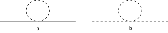
Figure 1: Loop contributions to the kaon (a) and pion (b) two-point functions. The continuous and dashed lines stand for kaon and pion propagators respectively. The relevant interactions are ${\cal L}^{(2)}_{\pi K}$ for the kaon and ${\cal L}^{(2)}_{\pi\pi}$ for the pion. Vertices from ${\cal L}^{(1)}_{\pi K}$ do not contribute. As explained in section 3, closed kaon-loops must not be taken into account.

$$M_{\pi}^{2} = m_{0}^{2}\left(1+2{m_{0}^{2}\over F^{2}}l_{3}^{r}+{m_{0}^{2}\over F^{2}}{\bar{\mu}}_{\pi}\right),$$

$$M_{{\mbox{\tiny$K$}}}^{2} = M^{2}+M^{(2)}m_{0}^{2}+M^{(4)}m_{0}^{4},$$ (12)

where

$$M^{(2)} = -2\sigma_{0},$$

$$M^{(4)} = 4\sigma_{0}(C_{5}^{r}+2C_{6}^{r})-8(C_{13}^{r}+C_{14}^{r}+2C_{15}^{r})-{3M^{2}A_{2}\over 256\pi^{2}F_{\pi}^{2}}$$

$$+{\bar{\mu}}_{\pi}\left({3A_{1}\over F_{\pi}^{2}}+{6\sigma_{0}\over F_{\pi}^{2}}+{3M^{2}A_{2}\over 4F_{\pi}^{2}}\right),$$

$$\sigma_{0} = A_{3}+2A_{4},$$

$${\bar{\mu}}_{\pi} = {1\over 32\pi^{2}}\ln{m_{0}^{2}\over\mu^{2}}.$$

Since the first two coefficients in the kaon-mass expansion are finite, the constants $M$ and $\sigma_{0}$ are not renormalised.

The pion decay constant has been calculated in [5] to fourth chiral order as

$$F_{\pi}=F\left(1+{m_{0}^{2}\over F^{2}}l_{4}^{r}-2{m_{0}^{2}\over F^{2}}{\bar{\mu}}_{\pi}\right).$$ (13)

This result is not modified because the effect of closed kaon loops is already included in the $\chi SU(2)$ coupling constants.

The kaon decay constant cannot be obtained in the present framework, because strangeness-changing, axial currents have not been coupled to external sources in the general $\chi SU(2)$ Lagrangian.

6.1 Matching with chiral $SU(3)$

In the $\chi SU(3)$ theory the strange-quark mass is treated as an expansion parameter, whereas in the $\chi SU(2)$ case it is fixed and contained in the low-energy constants, just like all the other heavy-quark masses. Comparing the expressions for $M_{\pi}$, $M_{{\mbox{\tiny$K$}}}$ and $F_{\pi}$, given by (6) and (13) respectively, with the corresponding $\chi SU(3)$ results [6] leads to expansions of the low-energy constants in powers of the strange-quark mass (${\bar{M}}_{K}^{2}=B_{0}m_{s}$):

$$M^{2} = {\bar{M}}_{K}^{2}+{{\bar{M}}_{K}^{4}\over F_{0}^{2}}\left[{1\over 36\pi^{2}}\ln({4{\bar{M}}_{K}^{2}\over 3\mu^{2}})-8(2L_{4}^{r}+L_{5}^{r}-4L_{6}^{r}-2L_{8}^{r})\right]+O({\bar{M}}_{K}^{6}),$$

$$\sigma_{0} = -{1\over 4}-{{\bar{M}}_{K}^{2}\over F_{0}^{2}}\left[{1\over 288\pi^{2}}+{1\over 72\pi^{2}}\ln({4{\bar{M}}_{K}^{2}\over 3\mu^{2}})-4(2L_{4}^{r}+L_{5}^{r}-4L_{6}^{r}-2L_{8}^{r})\right]+O({\bar{M}}_{K}^{4}),$$

$${F^{2}\over 8}(C_{5}^{r}+2C_{6}^{r})+F^{2}(C_{13}^{r}+C_{14}^{r}+C_{15}^{r})+{3M^{2}A_{2}\over 2048\pi^{2}}$$

$$= -{5\over 9216\pi^{2}}-{1\over 2304\pi^{2}}\ln({4{\bar{M}}_{K}^{2}\over 3\mu^{2}})+{1\over 4}(4L_{4}^{r}+L_{5}^{r}-8L_{6}^{r}-2L_{8}^{r})+O({\bar{M}}_{K}^{2}).$$

The combination of low-energy constants associated with the second order Lagrangian ${\cal L}_{\pi K}^{(2)}$,

$$A_{1}+{M^{2}A_{2}\over 4}={1\over 2}+O({\bar{M}}_{K}^{2}),$$

is evaluated to next-to-leading order in section (9).

The results for the expansions of pionic low-energy constants coincide with those given in [6] and are not repeated here.

7 Relativistic versus non-relativistic loops

Chiral-power counting is a non-trivial problem whenever particles are present whose masses do not vanish in the chiral limit. In baryon $\chi{\rm PT}$ there are three main approaches to the calculation of the scattering amplitude to third chiral order [9, 19, 24]. The relativistic approach [9] maintains relativistic invariance during the whole calculation and uses the same techniques of dimensional regularisation that are used in standard $\chi{\rm PT}$ with (pseudo-) Goldstone bosons only. The chiral power $D$ of the non-polynomial part of a given loop diagram without closed nucleon loops is given by

$$D=2L+1+\sum_{d}(d-2)N^{M}_{d}+\sum_{d}(d-1)N^{MN}_{d}$$ (14)

where $L$ is the number of loops and $N^{M}_{d}$($N^{MN}_{d}$) the number of pure meson (meson-nucleon) vertices, whose tree contributions are of chiral order $d$. However, loop diagrams usually contain also terms of lower order than $D$. Although these terms can be absorbed into the low-energy constants, most applications to pion-nucleon scattering are performed in the ‘non-relativistic’ approach (${\rm HB}\chi{\rm PT}$).

In ${\rm HB}\chi{\rm PT}$ [24] the Lorentz-invariant Lagrange density is written as a sum of terms, which break in general Lorentz invariance, and loop calculations are performed using these non-invariant vertices. In this approach the spin structure is simplified and the power-counting formula (14) can easily be proved. Lorentz invariance can be recovered at a later stage but there are many more vertices than in the relativistic case. Furthermore ${\rm HB}\chi{\rm PT}$ suffers from a deficiency: The perturbation series corresponding to the non-relativistic expansion fails to converge in part of the low-energy region [20].

An alternative to the above method is used in [19], where the heavy-particle expansion is used only under the loop integral and not – as in ${\rm HB}\chi{\rm PT}$ – on the Lagrangian level. This method is relativistic at every stage of the calculation and the power-counting formula (14) is also valid for the divergent part. Although this method suffers in general from the same deficiency as ${\rm HB}\chi{\rm PT}$ it seems to be the most efficient one for pion-kaon scattering to one loop because in that case – due to the absence of cubic interaction terms – there are no such low-energy divergencies as those mentioned above in the case of ${\rm HB}\chi{\rm PT}$. This is shown explicitely in appendix E.

8 The scattering amplitude

The isospin $3/2$ amplitude is defined by

$${}_{\rm out}\langle\,\pi^{+}(\vec{p}_{3})K^{+}(\vec{p}_{4})|\pi^{+}(\vec{p}_{1})K^{+}(\vec{p}_{2})\,\rangle_{\rm in}={\rm i}(2\pi)^{4}\delta^{(4)}(p_{1}+p_{2}-p_{3}-p_{4})T^{3\over 2}(s,t,u).$$

where $s,u$ and $t$ are the conventional Mandelstam variables,

$$s = (p_{1}+p_{2})^{2},$$

$$u = (p_{1}-p_{4})^{2},$$

$$t = (p_{1}-p_{3})^{2},$$

subject to the constraint $s+u+t=2(M_{\pi}^{2}+M_{{\mbox{\tiny$K$}}}^{2})$. The isospin ${1\over 2}$ amplitude can be obtained from $T^{3/2}$ by $s\leftrightarrow u$ crossing:

$$T^{1/2}(s,t,u)={3\over 2}T^{3/2}(u,t,s)-{1\over 2}T^{3/2}(s,t,u).$$

It is useful to define the amplitudes

$$T^{+}(s,t,u) = {1\over 3}\left(T^{1/2}(s,t,u)+2T^{3/2}(s,t,u)\right),$$ (15)

$$T^{-}(s,t,u) = {1\over 3}\left(T^{1/2}(s,t,u)-T^{3/2}(s,t,u)\right),$$ (16)

where $T^{+}$($T^{-}$) is even (odd) under $s\leftrightarrow u$ crossing. In the $s$-channel the decomposition into partial waves is given by

$$T^{I}(s(q),t(q,z))=16\pi\sum_{l=0}^{\infty}(2l+1)t_{l}^{I}(q)P_{l}(z).$$ (17)

In the expansion of the amplitude to fourth chiral order, only the first three Legendre polynomials $P_{l}$ are needed:

$$P_{0}(z) = 1,$$

$$P_{1}(z) = z,$$

$$P_{2}(z) = {1\over 2}(3z^{2}-1).$$

The dependence of $s$ and $t$ on the momentum $q$ of center of mass and the scattering angle $\theta$ is given by

$$s(q) = \left(\sqrt{M_{\pi}^{2}+q^{2}}+\sqrt{M_{{\mbox{\tiny$K$}}}^{2}+q^{2}}\right)^{2},$$

$$t(q,z) = -2q^{2}(1-z),$$

$$z = \cos\theta.$$

In the elastic region, the partial-wave amplitudes satisfy the unitarity constraint

$${\rm Im}\,t_{l}^{I}={2q\over\sqrt{s}}\arrowvert t_{l}^{I}\arrowvert,$$ (18)

and close to the threshold the Taylor coefficients of their real parts define the scattering lengths $a$, effective ranges $b$,…:

$${\rm Re}\,t_{l}^{I}(q)={\sqrt{s(q)}\over 2}q^{2l}\left(a_{l}^{I}+b_{l}^{I}q^{2}+c_{l}^{I}q^{4}+O(q^{6})\right).$$ (19)

8.1 Evaluation of Feynman diagrams

For the calculation of the off-shell scattering amplitude it would be necessary to evaluate the general form of the matrix elements of two axial currents (or pseudoscalar densities) between two kaon states. Here we are only interested in the on-shell amplitude and, as explained in [25], the standard techniques of Feynman diagrams can be used: all external sources are turned off in the general Lagrangian (5.1) and the traces of the matrix fields (6) are developed up to the sixth power in the physical meson fields. As in the $\chi SU(3)$ theory there are only three different types of Feynman diagrams at the one-loop level. These are shown in figure 2. Tree diagrams must be evaluated using all the vertices of the complete fourth order Lagrangian. The tadpole contributions are proportional to the pion propagator at $x=0$:

$${1\over{\rm i}}\Delta_{\pi}(0) = 2M_{\pi}^{2}\lambda+2M_{\pi}^{2}{\bar{\mu}_{\pi}},$$

$$\lambda = {\mu^{d-4}\over 16\pi^{2}}\left({1\over d-4}-{1\over 2}\left(\ln 4\pi+\Gamma^{\prime}(1)+1\right)\right),$$

$${\bar{\mu}_{\pi}} = {1\over 32\pi^{2}}\ln{M_{\pi}^{2}\over\mu^{2}}.$$

and their chiral order $D$ is given by $D=D_{\rm tree}+2$ where $D_{\rm tree}$ denotes the chiral order of the tree contribution of the same vertex. In order to obtain the scattering amplitude to fourth chiral order, vertices from ${\cal L}_{\pi K}^{(1)}$ and ${\cal L}_{\pi K}^{(2)}$ must be taken into account. Remember that closed kaon loops are not calculated in this approach, because such contributions are considered to be already included in the coupling constants (see section 3).

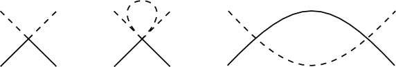
Figure 2: Tree, tadpole and fish diagram. The continuous and dashed lines stand for kaon and pion propagators respectively. Crossed fish-diagrams are not shown.

There are five different fish diagrams contributing to the amplitude according to the five different combinations of particles running in the loop. These combinations are: $\pi^{0}$–$\pi^{0}$ ($t$-channel), $\pi^{\pm}$–$\pi^{\mp}$ ($t$-channel), $K^{0}$–$\pi^{0}$ ($u$-channel), $K^{+}$–$\pi^{+}$ ($s$-channel) and $K^{\pm}$–$\pi^{\mp}$ ($u$-channel). Figure 2 shows the $s$-channel $K^{+}$–$\pi^{+}$ diagram which is proportional to

$$J_{K\pi}(s)={1\over{\rm i}}\int{{\rm d}^{d}l\over(2\pi)^{d}}{1\over M_{\pi}^{2}-l^{2}}{1\over M_{K}^{2}-(p-l)^{2}},$$

where $p=p_{1}+p_{2}$ is the total momentum.

The function $J_{K\pi}(s)$ is Lorentz-invariant and can therefore be evaluated at any $p^{\prime}=\Lambda p$ where $\Lambda$ is an element of the Lorentz group. It is expedient to choose the Lorentz transformation such that the initial kaon momentum $p_{2}$ is just $p_{2}=M_{K}v$, with $v=(1,0,0,0)$, and to develop the kaon propagator under the integral sign. The $M_{{\mbox{\tiny$K$}}}^{2}$ terms in the denominator then cancel and in this heavy kaon HK formalism the function $J_{K\pi}$ becomes

$$J_{K\pi}^{HK}(s) = -{1\over 2{\rm i}M_{{\mbox{\tiny$K$}}}}\int{{\rm d}^{d}l\over(2\pi)^{d}}{1\over M_{\pi}^{2}-l^{2}}{1\over v(p_{1}-l)}\left(1-{(p_{1}-l)^{2}\over 2M_{{\mbox{\tiny$K$}}}v(p_{1}-l)}+O(l^{2})\right).$$

This integral starts contributing at $O(p^{1})$ and the two vertices in the fish diagram must therefore be taken from ${\cal L}_{\pi K}^{(m)}$ and ${\cal L}_{\pi K}^{(n)}$ with $m+n\leq 3$. This confirms the general power-counting formula (14). It is shown explicitly in appendix E that the power series resulting from the development of the kaon propagator converges to the correct result.

The expression (8.1) can be written as a sum of standard integrals of heavy-baryon $\chi{\rm PT}$:

$$J_{K\pi}^{HK}(s)={1\over 2M_{{\mbox{\tiny$K$}}}}J_{0}(\omega)+{1\over 4M_{{\mbox{\tiny$K$}}}^{2}}(M_{\pi}^{2}G_{0}(\omega)-2\omega G_{1}(\omega)+dG_{2}(\omega)+G_{3}(\omega))$$

where

$$\omega={s-M_{{\mbox{\tiny$K$}}}^{2}-M_{\pi}^{2}\over 2M_{{\mbox{\tiny$K$}}}}={p_{1}p_{2}\over M_{{\mbox{\tiny$K$}}}}.$$

The functions $J_{i}$ and $G_{i}$ for $(i=0,1,2)$ are taken from [24] and [26] and are given in appendix B.

Posing $\nu=s-u$, which differs from the conventional definition, the full fourth order amplitude is given by

$$T^{3\over 2} = T^{3\over 2}_{1}+T^{3\over 2}_{2}+T^{3\over 2}_{3}+T^{3\over 2}_{4},$$

$$T^{3\over 2}_{1} = -{\nu\over 4F_{\pi}^{2}},$$

$$T^{3\over 2}_{2} = t{A_{1}\over 2F_{\pi}^{2}}-\nu^{2}{{A_{2}}\over 16F_{\pi}^{2}}-M_{\pi}^{2}\left({A_{1}\over F_{\pi}^{2}}+{{2\rho}\over F_{\pi}^{2}}\right),$$

$$T^{3\over 2}_{3} = {\nu^{2}\over{16F_{\pi}^{4}}}\left[f_{s}(\nu,t)+3f_{u}(\nu,t)\right]+{\bar{J}}_{\pi\pi}(t)\left({{M_{\pi}^{2}\nu}\over 6F_{\pi}^{2}}-{{t\nu}\over 24F_{\pi}^{2}}\right)+{\bar{\mu}}_{\pi}\left({{t\nu}\over{12F_{\pi}^{4}}}+{\nu^{3}\over{16F_{\pi}^{4}M_{{\mbox{\tiny$K$}}}^{2}}}\right)$$

$$+\nu^{3}\left({B_{2}^{r}\over 32F_{\pi}^{2}}-{1\over{512\pi^{2}F_{\pi}^{4}M_{{\mbox{\tiny$K$}}}^{2}}}\right)+t\nu\left(-{B_{1}^{r}\over 4F_{\pi}^{2}}+{1\over{384\pi^{2}F_{\pi}^{4}}}\right)$$

$$+M_{\pi}^{2}\nu\left({B_{1}^{r}-4B_{3}^{r}\over 2F_{\pi}^{2}}-{1\over 96\pi^{2}F_{\pi}^{4}}\right),$$

$$T^{3\over 2}_{4} = f_{s}(\nu,t)\left[-{{t\nu}\over{8F_{\pi}^{4}}}+M_{\pi}^{2}\nu\left({1\over{4F_{\pi}^{4}}}+{\rho\over F_{\pi}^{4}}\right)+\nu^{3}\left(-{1\over{64F_{\pi}^{4}M_{{\mbox{\tiny$K$}}}^{2}}}+{A_{1}\over{32F_{\pi}^{4}M_{{\mbox{\tiny$K$}}}^{2}}}+{A_{2}\over{32F_{\pi}^{4}}}\right)\right]$$ (21)

$$+f_{u}(\nu,t)\left[{{3t\nu}\over{8F_{\pi}^{4}}}+M_{\pi}^{2}\nu\left(-{3\over{4F_{\pi}^{4}}}+{\rho\over F_{\pi}^{4}}\right)+\nu^{3}\left({3\over{64F_{\pi}^{4}M_{{\mbox{\tiny$K$}}}^{2}}}+{A_{1}\over{32F_{\pi}^{4}M_{{\mbox{\tiny$K$}}}^{2}}}+{A_{2}\over{32F_{\pi}^{4}}}\right)\right]$$

$$+{\bar{J}}_{\pi\pi}(t)\left[t^{2}\left({A_{1}\over{2F_{\pi}^{4}}}+{{M_{{\mbox{\tiny$K$}}}^{2}A_{2}}\over{12F_{\pi}^{4}}}\right)+M_{\pi}t\left(-{{5A_{1}}\over{4F_{\pi}^{4}}}-{{3M_{{\mbox{\tiny$K$}}}^{2}A_{2}}\over{8F_{\pi}^{4}}}-{{2\rho}\over F_{\pi}^{4}}\right)\right.$$

$$+\left.M_{\pi}^{4}\left({A_{1}\over{2F_{\pi}^{4}}}+{{M_{{\mbox{\tiny$K$}}}^{2}A_{2}}\over{6F_{\pi}^{4}}}+{\rho\over F_{\pi}^{4}}\right)\right]$$

$$+\lambda_{(\nu^{4})}\nu^{4}+\lambda_{(\nu^{2}t)}\nu^{2}t+\lambda_{(t^{2})}t^{2}+\lambda_{(\nu^{2}m^{2})}\nu^{2}M_{\pi}^{2}+\lambda_{(tm^{2})}tM_{\pi}^{2}+\lambda_{(m^{4})}M_{\pi}^{4},$$

where

$$\rho=\sigma_{0}\left[1-2m_{0}^{2}(C_{5}^{r}+2C_{6}^{r})\right]+O(m_{0}^{4}).$$

The loop functions are given in terms of the variables $\nu$ and $t$ by

$$f_{s}(\nu,t) = \left({1\over 32\pi^{2}}-{\nu\over 64\pi^{2}M_{{\mbox{\tiny$K$}}}^{2}}\right)\sqrt{{(t-\nu)^{2}\over M_{{\mbox{\tiny$K$}}}^{4}}-16{M_{\pi}^{2}\over M_{{\mbox{\tiny$K$}}}^{2}}}\left[{\rm i}\pi-{\rm arccosh}\left({\nu-t\over 4M_{{\mbox{\tiny$K$}}}M_{\pi}}\right)\right],$$

$$f_{u}(\nu,t) = \left({1\over 32\pi^{2}}+{\nu\over 64\pi^{2}M_{{\mbox{\tiny$K$}}}^{2}}\right)\sqrt{{(t+\nu)^{2}\over M_{{\mbox{\tiny$K$}}}^{2}}-16{M_{\pi}^{2}\over M_{{\mbox{\tiny$K$}}}^{2}}}{\rm arccosh}\left({\nu+t\over 4M_{{\mbox{\tiny$K$}}}M_{\pi}}\right),$$

$${\bar{J}}_{\pi\pi}(t) = {1\over 16\pi^{2}}\left(\sigma(t)\ln{\sigma(t)-1\over\sigma(t)+1}+2\right),\hskip 19.91692pt(t\leq 0),$$

$$\sigma(t) = \sqrt{1-{4M_{\pi}^{2}\over t}}.$$

In the physical energy region $\nu+t\geq 4M_{{\mbox{\tiny$K$}}}M_{\pi}$ and $t\leq 0$. The constants $A_{1}$, $A_{2}$, and $\sigma_{0}$ are scale-independent as are the combinations $\lambda_{(pol)}$ of low-energy constants which are defined in appendix C. It is easy to see whether a given term in the scattering amplitude (8.1), arises from a tree or a loop diagram: loop contributions carry a factor $\pi^{2}$ in the denominator. As a consistency check we have verified that the partial-wave amplitudes $t^{I}_{l}$, defined by equation (17), satisfy the unitarity constraint (18).

9 Comparison with the chiral $SU(3)$ amplitude

A numerical estimate of the low-energy constants can be obtained by comparing the above amplitude with the corresponding amplitude of the $\chi SU(3)$ theory which is given in [8] and whose result is based on the generating functional given in [6]. The standard method of Feynman diagrams leads to the same result. The amplitude involves loop functions of heavy particles ($P,Q\in\{K,\eta\}$),

$$M_{PQ}^{r}(s) = {1\over 12s}(s-2\Sigma){\bar{J}}_{PQ}(s)+{\Delta^{2}\over 3s^{2}}\;\bar{\bar{J}}\!_{PQ}(s)-{1\over 6}k_{PQ}+{1\over 288\pi^{2}},$$

$$L_{PQ} = {\Delta^{2}\over 4s}{\bar{J}}_{PQ},\qquad K_{PQ}={\Delta\over 2s}{\bar{J}}_{PQ},$$

$$k_{PQ} = {1\over 32\pi^{2}}{M_{P}^{2}\ln(M_{P}^{2}/\mu^{2})-M_{Q}^{2}\ln(M_{Q}^{2}/\mu^{2})\over M_{P}^{2}-M_{Q}^{2}},$$

$$\;\bar{\bar{J}}\!_{PQ}(s) = {\bar{J}}(s)-s{\bar{J}}^{\prime}(0),\qquad{\bar{J}}^{\prime}(0)={1\over 32\pi^{2}}\left({\Sigma\over\Delta^{2}}+2{M_{P}^{2}M_{Q}^{2}\over\Delta^{3}}\ln{M_{Q}^{2}\over M_{P}^{2}}\right),$$

$${\bar{J}}_{PQ}(s) = {1\over 32\pi^{2}}\left(2+{\Delta\over s}\ln{M_{Q}^{2}\over M_{P}^{2}}-{\Sigma\over\Delta}\ln{M_{Q}^{2}\over M_{P}^{2}}-{\nu\over s}\ln{(s+\nu)^{2}-\Delta^{2}\over(s-\nu)^{2}-\Delta^{2}}\right),$$

$$\Sigma = \Sigma_{PQ}=M_{P}^{2}+M_{Q}^{2},\qquad\Delta=\Delta_{PQ}=M_{P}^{2}-M_{Q}^{2},$$

which, close to the threshold, give real contributions to the scattering amplitude and can be developed in powers of $M_{\pi}$, $t$ and $\nu=s-u$. For example, the function ${\bar{J}}_{\eta,K}$ is needed to third $SU(2)$ order:

$${\bar{J}}_{\eta K}(u)=$$

$${1\over\pi^{2}}\left({1\over 16}+{\nu\over 32M_{0}^{2}}-{m_{0}^{2}\over 8M_{0}^{2}}+{t\over 32M_{0}^{2}}+{13\nu^{2}\over 1024M_{0}^{4}}-{27m_{0}^{2}\nu\over 512M_{0}^{4}}+{13t\nu\over 512M_{0}^{4}}+{83\nu^{3}\over 16384M_{0}^{6}}\right)$$

$$-{\arctan(\sqrt{2})\over\sqrt{2}\pi^{2}}\left({1\over 6}+{5\nu\over 96M_{0}^{2}}-{11m_{0}^{2}\over 96M_{0}^{2}}+{5t\over 96M_{0}^{2}}+{53\nu^{2}\over 3072M_{0}^{4}}-{35m_{0}^{2}\nu\over 512M_{0}^{4}}+{53t\nu\over 1536M_{0}^{4}}+{343\nu^{3}\over 49152M_{0}^{6}}\right)$$

$$+{\ln(4/3)\over\pi^{2}}\left({5\over 24}-{\nu\over 192M_{0}^{2}}+{5m_{0}^{2}\over 24M_{0}^{2}}-{t\over 192M_{0}^{2}}-{\nu^{2}\over 384M_{0}^{4}}+{m_{0}^{2}\nu\over 64M_{0}^{4}}-{t\nu\over 192M_{0}^{4}}-{\nu^{3}\over 768M_{0}^{6}}\right),$$

$$\mbox{where}\hskip 56.9055ptM_{0}^{2} = B_{0}(m_{s}+{\hat{m}}),$$

$$m_{0}^{2} = 2B_{0}{\hat{m}}.$$

If the two heavy masses are equal, $M_{P}=M_{Q}$, the functions ${\bar{J}}_{PP}$ and the constants $k_{PP}$ simplify to

$${\bar{J}}_{PP}(t) = {t\over 96\pi^{2}M_{P}^{2}}+{t^{2}\over 960\pi^{2}M_{P}^{4}}+O(t^{3}),$$

$$k_{PP} = {1\over 32\pi^{2}}\left(\ln{M_{P}^{2}\over\mu^{2}}+1\right).$$

Note that $K$–$K$- and $\eta$–$\eta$-loops can only contribute in the $t$-channel.

If both amplitudes are developed in powers of $t$, $\nu$ and ${\hat{m}}$, an expansion of the $\chi SU(2)$ constants in powers of the strange-quark mass is obtained (see appendix D).

10 Threshold parameters

The formulae (8.1) specify the scattering amplitude to fourth chiral order. The expression involves 12 combinations of low-energy constants which can be related to 12 threshold parameters defined by equation (19). These observables are $a^{I}_{0}$, $b^{I}_{0}$, $c^{I}_{0}$, $a^{I}_{1}$, $b^{I}_{1},$ and $a^{I}_{2}$ for $I\in\{1/2,3/2\}$. For $x\in\{a,b,c\}$ and $l\in\{0,1,2\}$ we define

$$x^{+}_{l} = x^{1/2}_{l}+2x^{3/2}_{l}$$

$$x^{-}_{l} = x^{1/2}_{l}-x^{3/2}_{l},$$ (23)

after which it is straightforward to extract these threshold parameters from the amplitude.

10.1 Corrections to current algebra and a low-energy theorem

The threshold parameters $x^{-}_{l}$ can also be extracted from the amplitude $T^{-}_{l}(\nu,t)$ which is odd in $\nu$ and which therefore contains the polynomials of first and third chiral order ($\nu$, $\nu t$, $\nu M_{\pi}^{2}$, $\nu^{3}$). Chiral invariance ensures that the lowest-order polynomial proportional to $\nu$ is parameter-free, as are the leading terms of some of the threshold parameters $x^{-}_{l}$. Here only $a_{0}^{-}$, $a_{2}^{-}$ and $b_{1}^{-}$ are listed and the parameters $a_{1}^{-}$, $b_{0}^{-}$ and $c_{0}^{-}$ are given in appendix F.

$$a^{-}_{0} = {M_{\pi}\over M_{{\mbox{\tiny$K$}}}+M_{\pi}}{3M_{{\mbox{\tiny$K$}}}\over 8\pi F_{\pi}^{2}}$$

$$+{M_{\pi}^{3}\over M_{{\mbox{\tiny$K$}}}+M_{\pi}}\left({M_{{\mbox{\tiny$K$}}}\over 16\pi^{3}F_{\pi}^{4}}-{3B_{1}^{r}M_{{\mbox{\tiny$K$}}}\over 4\pi F_{\pi}^{2}}-{3B_{2}^{r}M_{{\mbox{\tiny$K$}}}^{3}\over 4\pi F_{\pi}^{2}}+{3B_{3}^{r}M_{{\mbox{\tiny$K$}}}\over\pi F_{\pi}^{2}}-{3M_{{\mbox{\tiny$K$}}}{\bar{\mu}}_{\pi}\over 2\pi F_{\pi}^{4}}\right),$$

$$b^{-}_{1} = {1\over M_{\pi}(M_{{\mbox{\tiny$K$}}}+M_{\pi})}\left(-{1\over 32\pi F_{\pi}^{2}M_{{\mbox{\tiny$K$}}}}-{37M_{{\mbox{\tiny$K$}}}\over 11520\pi^{3}F_{\pi}^{4}}+{B_{1}^{r}M_{{\mbox{\tiny$K$}}}\over 8\pi F_{\pi}^{2}}-{M_{{\mbox{\tiny$K$}}}{\bar{\mu}}_{\pi}\over 24\pi F_{\pi}^{4}}\right)$$ (24)

$$+{1\over M_{{\mbox{\tiny$K$}}}+M_{\pi}}\left(-{85\over 2304\pi^{3}F_{\pi}^{4}}-{B_{1}^{r}\over 8\pi F_{\pi}^{2}}-{3B_{2}^{r}M_{{\mbox{\tiny$K$}}}^{2}\over 8\pi F_{\pi}^{2}}-{17{\bar{\mu}}_{\pi}\over 24\pi F_{\pi}^{4}}\right),$$

$$a^{-}_{2} = {1\over M_{\pi}(M_{{\mbox{\tiny$K$}}}+M_{\pi})}{M_{{\mbox{\tiny$K$}}}\over 4800\pi^{3}F_{\pi}^{4}}+{1\over M_{{\mbox{\tiny$K$}}}+M_{\pi}}\left(-{1\over 1152\pi^{3}F_{\pi}^{4}}+{B_{1}^{r}\over 20\pi F_{\pi}^{2}}-{{\bar{\mu}}_{\pi}\over 60\pi F_{\pi}^{4}}\right).$$

It is interesting that loop corrections (factor $\pi^{3}$ in the denominator) to $b_{1}^{-}$ have the same chiral order as the tree contribution of lowest order, and the $d$-wave scattering length $a_{2}^{-}$ is even dominated by a loop contribution. This happens because in the definition of these observables (see equation (19)) a factor $q^{l}$ has to be extracted, which in general leads to factors of $M_{\pi}$ in the denominator. For the same reason, tree contributions from the third-order Lagrangian are less suppressed in $b_{1}^{-}$ and $a_{2}^{-}$ and these observables are therefore the natural candidates to replace the unknown coupling constants $B_{1}^{r}$ and $B_{2}^{r}$ in the expressions for the four other observables. The remaining low-energy constant $B_{3}^{r}$ corresponds to a chiral-symmetry breaking term and therefore cannot be extracted from the angular and energy distributions of the scattering cross section. However, the theoretical estimate from appendix D,

$$B_{3}^{r}(\mu=770)=7.9\cdot 10^{-7}\hskip 2.84526pt{\rm MeV}^{-2},$$

gives parameterless corrections to the ‘current algebra’ result of the observables $a_{0}^{-}$, $b_{0}^{-}$, $a_{1}^{-}$ and $c_{0}^{-}$. Here only $a_{0}^{-}$ is listed. The parameters $a_{1}^{-}$ and $b_{0}^{-}$ are given in appendix F.

$$a^{-}_{0} = {M_{\pi}\over M_{{\mbox{\tiny$K$}}}+M_{\pi}}\left({3M_{{\mbox{\tiny$K$}}}\over 8\pi F_{\pi}^{2}}+{M_{{\mbox{\tiny$K$}}}^{3}\over 960\pi^{3}F_{\pi}^{4}}\right)+{M_{\pi}^{2}\over M_{{\mbox{\tiny$K$}}}+M_{\pi}}\left({1\over 16\pi F_{\pi}^{2}}+{M_{{\mbox{\tiny$K$}}}^{2}\over 240\pi^{3}F_{\pi}^{4}}-5M_{{\mbox{\tiny$K$}}}^{3}a_{2}^{-}\right)$$ (25)

$$+{M_{\pi}^{3}\over M_{{\mbox{\tiny$K$}}}+M_{\pi}}\left({3B^{r}_{3}M_{{\mbox{\tiny$K$}}}\over\pi F_{\pi}^{2}}+{49M_{{\mbox{\tiny$K$}}}\over 384\pi^{3}F_{\pi}^{4}}-{M_{{\mbox{\tiny$K$}}}{\bar{\mu}}_{\pi}\over 4\pi F_{\pi}^{4}}-15M_{{\mbox{\tiny$K$}}}^{2}a_{2}^{-}+2M_{{\mbox{\tiny$K$}}}^{2}b_{1}^{-}\right)$$

$$+{M_{\pi}^{4}\over M_{{\mbox{\tiny$K$}}}+M_{\pi}}\left(-10M_{{\mbox{\tiny$K$}}}a_{2}^{-}+2M_{{\mbox{\tiny$K$}}}b_{1}^{-}\right).$$

The only input from $\chi SU(3)$ is the constant $B^{r}_{3}$, which appears in the term of $O(p^{3})$.

Another interesting combination between scattering lengths is

$$A^{-}=a_{0}^{-}-6M_{\pi}M_{{\mbox{\tiny$K$}}}a_{1}^{-}+30M_{\pi}^{2}M_{{\mbox{\tiny$K$}}}^{2}a_{2}^{-},$$

which is discussed (in the $\chi SU(3)$ current algebra (CA) approach) by Lang [3]. Without taking into account loop corrections

$$A^{-}_{CA}=0.$$

From the results (10.1) and (F) one finds

$$A^{-} = {M_{\pi}\over M_{{\mbox{\tiny$K$}}}+M_{\pi}}{M_{{\mbox{\tiny$K$}}}^{3}\over 160\pi^{3}F_{\pi}^{4}}+{M_{\pi}^{3}\over M_{{\mbox{\tiny$K$}}}+M_{\pi}}\left({3M_{{\mbox{\tiny$K$}}}\over 32\pi^{3}F_{\pi}^{4}}+{3B_{2}^{r}M_{{\mbox{\tiny$K$}}}^{3}\over 2\pi F_{\pi}^{2}}+{3M_{{\mbox{\tiny$K$}}}{\bar{\mu}}_{\pi}\over\pi F_{\pi}^{4}}\right),$$

valid to fourth chiral order. The chiral-symmetry breaking terms (proportional to $B_{3}^{r}$) cancel in this sum. The first- and the third-order loop corrections are $0.009M_{\pi}^{-1}$ and $0.011M_{\pi}^{-1}$ respectively. The correction from the polynomial $\nu^{3}$ – which is of $\chi SU(3)$ order $p^{6}$ – can be estimated with the $\chi SU(3)$ value for $B_{2}^{r}$ and is about 10 % of the loop corrections. This leads to

$$A^{-}=0.022M_{\pi}^{-1}.$$

Alternatively, the unknown constant $B_{2}^{r}$ can be expressed in terms of the observables $a_{2}^{-}$ and $b_{1}^{-}$,

$$A^{-} = {M_{\pi}\over M_{{\mbox{\tiny$K$}}}+M_{\pi}}{M_{{\mbox{\tiny$K$}}}^{3}\over 240\pi^{3}F_{\pi}^{4}}+{M_{\pi}^{2}\over M_{{\mbox{\tiny$K$}}}+M_{\pi}}\left(-{1\over 8\pi F_{\pi}^{2}}+10M_{{\mbox{\tiny$K$}}}^{3}a_{2}^{-}-{M_{{\mbox{\tiny$K$}}}^{2}\over 480\pi^{3}F_{\pi}^{4}}\right)$$ (26)

$$-{M_{\pi}^{3}M_{{\mbox{\tiny$K$}}}\over M_{{\mbox{\tiny$K$}}}+M_{\pi}}\left(4M_{{\mbox{\tiny$K$}}}b_{1}^{-}+{1\over 16\pi^{3}F_{\pi}^{4}}\right)-{M_{\pi}^{4}M_{{\mbox{\tiny$K$}}}\over M_{{\mbox{\tiny$K$}}}+M_{\pi}}\left(10a_{2}^{-}+4b_{1}^{-}\right),$$

giving a result which is exact to fourth $\chi SU(2)$ order and which involves no low-energy constants.

Table 2 shows the numerical values obtained by using $\chi SU(3)$ estimates for $B_{1}^{r}$, $B_{2}^{r}$ and $B_{3}^{r}$ in (10.1) and (F), given in the appendix. Some experimental values for $a_{0}^{-}$ are given in table 3. More accurate data on threshold parameters of higher order would be needed to test relations (25), (26) and (F).

Table 2: Threshold parameters associated with the amplitude $T^{-}$. There are tree (CA) and loop contributions (loops) from ${\cal L}_{\pi{\mbox{\tiny$K$}}}^{(1)}$. The total result ($\chi SU(2)+\chi SU(3)$) also contains polynomial contributions from ${\cal L}_{\pi{\mbox{\tiny$K$}}}^{(3)}$, with low-energy constants estimated from $\chi SU(3)$ at a renormalisation scale of $\mu=770{\rm MeV}$.

thresh. param.	CA	loops	$\chi SU(2)+\chi SU(3)$
$a_{0}^{-}M_{\pi}$	0.20	0.01	$0.23\pm 0.01$
$b_{0}^{-}M_{\pi}^{3}$	0.10	0.01	$0.10\pm 0.01$
$c_{0}^{-}M_{\pi}^{5}$	-0.03	-0.01	$-0.052\pm 0.003$
$a_{1}^{-}M_{\pi}^{3}$	0.009	-0.001	$0.013\pm 0.002$
$b_{1}^{-}M_{\pi}^{5}$	-0.001	-0.001	$-0.002\pm 0.001$
$a_{2}^{-}M_{\pi}^{5}$	0	$2\cdot 10^{-5}$	$(20\pm 7)\cdot 10^{-5}$

The values for the scattering lengths are consistent with the result in [7], where the slope parameters $b_{0}^{1/2}$ and $b_{0}^{3/2}$, however, were obtained as

$$(b_{0}^{1/2})_{\scriptsize\cite[cite]{[\@@bibref{}{BKMthresh}{}{}]}}=(0.14\pm 0.02)M_{\pi}^{-3},\mbox{ }\quad(b_{0}^{3/2})_{\scriptsize\cite[cite]{[\@@bibref{}{BKMthresh}{}{}]}}=(-0.011\pm 0.005)M_{\pi}^{-3},$$ (27)

which is inconsistent with our result. In the $\chi SU(3)$ case $M_{\pi}/M_{{\mbox{\tiny$K$}}}$ is not a chiral expansion parameter and the analytical expressions for the threshold parameters are therefore more voluminous then in the $\chi SU(2)$ case. Thus only numerical values are given in [7].

Table 3: The scattering length $a_{0}^{-}$ as determined in various analyses. The values are in chronological order. The interval in the second column is chosen so as to cover the experimental results for $a^{(1/2)}_{0}$ [27] and $a^{(3/2)}_{0}$ [28]. References [29] and [30] are dispersion relation analyses based on more recent experiments, [16] and [15, 16] respectively, with much more data. The error in the second column is chosen so as to cover the results for $a^{(1/2)}_{0}$ and $a^{(3/2)}_{0}$ given in [29].

thresh. param.	before 1977	Karabarbounis [29]	Krivoruchenko [30]
$a_{0}^{-}M_{\pi}$	$0.2\dots 0.4$	$0.26\pm 0.06$	$0.22\pm 0.02$

10.2 Other parameter-free relations between threshold parameters

The amplitude $T^{+}_{l}$ is even in $\nu$ and it therefore involves the polynomials of second and fourth chiral order. In this case, chiral invariance does not restrict the associated threshold parameters, which are listed in appendix F.

The quantity $A^{+}$, defined by

$$A^{+} = a_{0}^{+}-M_{\pi}^{2}b_{0}^{+}+{3M_{\pi}^{3}\over 2M_{{\mbox{\tiny$K$}}}}\left(a_{1}^{+}+{b_{0}^{+}\over 4}\right)$$

$$+M_{\pi}^{4}\left[c_{0}^{+}-10a_{2}^{+}+\left({1\over 288\pi^{2}F_{\pi}^{2}}-{5\over 16M_{{\mbox{\tiny$K$}}}^{2}}\right)b_{0}^{+}-\left({1\over 48\pi^{2}F_{\pi}^{2}}+{9\over 8M_{{\mbox{\tiny$K$}}}^{2}}\right)a_{1}^{+}\right],$$

preserves chiral-power counting in the sense that no threshold parameter is needed to an unnaturally high precision. This quantity contains only (combinations of) coupling constants associated with chiral-symmetry breaking terms:

$$A^{+} = -{M_{\pi}^{2}\over M_{{\mbox{\tiny$K$}}}+M_{\pi}}{3\sigma_{0}\over 4\pi F_{\pi}^{2}}-{M_{\pi}^{3}\over M_{{\mbox{\tiny$K$}}}+M_{\pi}}{15\sigma_{0}\over 32\pi F_{\pi}^{2}M_{{\mbox{\tiny$K$}}}}$$ (28)

$$+{M_{\pi}^{4}\over M_{{\mbox{\tiny$K$}}}+M_{\pi}}\left({3\sigma_{0}\over 64\pi F_{\pi}^{2}M_{{\mbox{\tiny$K$}}}^{2}}+{3\sigma_{0}(C_{5}^{r}+2C_{6}^{r})\over 2\pi F_{\pi}^{2}}+{3\lambda_{(tm^{2})}\over 4\pi}+{3\lambda_{(m^{4})}\over 8\pi}+{\sigma_{0}\over 128\pi^{3}F_{\pi}^{4}}\right)$$

$$= (0.03\pm 0.02)M_{\pi}^{-1}+(0.006\pm 0.004)M_{\pi}^{-1}+(0.004\pm 0.006)M_{\pi}^{-1}$$

$$= (0.04\pm 0.03)M_{\pi}^{-1}.$$

The numerical values again result from theoretical $\chi SU(3)$ estimations of the $\chi SU(2)$ constants.

The same estimations can be used to obtain numerical values for the threshold parameters from expressions (F). However, due to the absence of parameter-free lowest-order predictions these values, shown in table 4, are less precise than those discussed in subsection 10.1.

The parameter

$$a_{1}^{(1/2)}=(a_{1}^{+}+2a_{1}^{-})/3=(0.018\pm 0.002)M_{\pi}^{-3}$$

is in very good agreement with the dispersion relation analysis of Karabarbounis and Shaw [29]:

$$0.0178M_{\pi}^{-3}\leq(a_{1}^{(1/2)})_{\scriptsize\cite[cite]{[\@@bibref{}{Karabarbounis}{}{}]}}\leq 0.0185M_{\pi}^{-3}.$$

Mean experimental values for $a_{0}^{1/2}$ and $a_{0}^{3/2}$ are given in [8]:

$$a_{0}^{1/2}=0.13\dots 0.24M_{\pi}^{-1},\quad a_{0}^{3/2}=-0.13\dots-0.05M_{\pi}^{-1}.$$

These were obtained long before the high-statistics experiment of [15] in 1988 which is an important reference for $\pi$–$K$ resonance data collected by the PDG [31]. The absence of precise experimental data for higher-order threshold parameters precludes the verification of relation (28).

Table 4: Threshold parameters associated with the amplitude $T^{+}$. Current algebra gives no contributions and loops must be considered form ${\cal L}_{\pi{\mbox{\tiny$K$}}}^{(1)}$ and ${\cal L}_{\pi{\mbox{\tiny$K$}}}^{(2)}$. The total result ($\chi SU(2)+\chi SU(3)$) contains in addition polynomial contributions from ${\cal L}_{\pi{\mbox{\tiny$K$}}}^{(2)}$ and ${\cal L}_{\pi{\mbox{\tiny$K$}}}^{(4)}$, with low-energy constants estimated from $\chi SU(3)$ .

thresh. param.	$\chi SU(2)+\chi SU(3)$
$a_{0}^{+}M_{\pi}$	$0.08\pm 0.04$
$b_{0}^{+}M_{\pi}^{3}$	$0.06\pm 0.03$
$c_{0}^{+}M_{\pi}^{5}$	$0.015\pm 0.004$
$a_{1}^{+}M_{\pi}^{3}$	$0.023\pm 0.008$
$b_{1}^{+}M_{\pi}^{5}$	$0.003\pm 0.002$
$a_{2}^{+}M_{\pi}^{5}$	$(4\pm 3)\cdot 10^{-4}$

As in the case of $T_{\pi K}^{-}$, the scattering lengths are consistent with the result of [7], whereas, as can be seen from equation (27) and definition (10), the effective range parameter $b_{0}^{+}$ is half the size. This cannot be due to the fact that the authors of [7] use older values for the $\chi SU(3)$ constants, since the effect of this would be too small. In the $\chi SU(3)$ case, our calculation of the $T_{\pi K}^{3/2}$ amplitude coincides exactly with the one in [8].

11 Summary and Conclusion

To the best of our knowledge, this is the first analysis of the threshold structure of pion-kaon scattering using only $\chi SU(2)$ symmetry of the strong interactions. Chiral $SU(2)$ symmetry is less strongly broken in nature than $\chi SU(3)$ symmetry and the chiral expansion is therefore expected to converge more rapidly. Chiral $SU(2)$ symmetry only allows for one interaction term of $O(p^{1})$,

$${\cal L}^{(1)}_{\pi,K}=D_{\mu}K^{+}D^{\mu}K-M^{2}K^{+}K,$$

where $D_{\mu}K=\partial_{\mu}K+\Gamma_{\mu}K$ is the covariant derivative containing the pion field (definition 4.1).

The lowest-order contribution to the isospin $3/2$ scattering amplitude is therefore parameter-free:

$$T^{3\over 2}_{1}=-{\nu\over 4F_{\pi}^{2}},$$

where $\nu=s-u$ contains indeed a term proportional to the pion mass and is therefore of first chiral order. The lowest-order contributions to the threshold parameters do not differ significantly from those given by the $\chi SU(3)$ current algebra result [3].

The isospin $3/2$ amplitude was calculated to fourth chiral order in the isospin limit and without including elecromagnetic interactions. The result is given by equation (8.1).

The loop correction to the current algebra result for the scattering length $a_{0}^{-}$ amounts to $5\%$ at a renormalisation scale of $\mu=770{\rm MeV}$. The loop contributions to the parameters $b_{0}^{-}$, $c_{0}^{-}$, $a_{1}^{-}$, $b_{1}^{-}$ and $a_{2}^{-}$ are given in table 2. The exact result for theses observables – valid to fourth chiral order – involves three unknown low-energy constants, $B_{1}^{r}$, $B_{2}^{r}$ and $B_{3}^{r}$. The observables $b^{-}_{1}$ and $a^{-}_{2}$ measure the first two constants so that a theoretical estimate (from chiral $SU(3)$ symmetry) of the “symmetry-breaking constant” $B_{3}^{r}$ produces parameter-free predictions for $a^{-}_{0}$, $b^{-}_{0}$ and $a^{-}_{1}$. These relations are given by formulae (25) and (F). There is also a pure $\chi SU(2)$ low-energy theorem – given by formula (26) – involving the above observables.

The $\nu$-even amplitude $T_{\pi K}^{+}$ starts at second chiral order and the associated threshold parameters $a^{+}_{0}$, $b^{+}_{0}$, $c^{+}_{0}$, $a^{+}_{1}$, $b^{+}_{1}$ and $a^{+}_{2}$ are not restricted by chiral $SU(2)$ symmetry. However, there are relations between these observables involving only $\chi SU(2)$ constants associated with a chiral-symmetry-breaking term. Equation (28) shows the result when all these constants are estimated from $\chi SU(3)$.

The relations between threshold parameters (25, 26, 28 and F), valid to fourth chiral ($SU(2)$) order, are the main result of the present analysis and could not have been obtained within $\chi SU(3)$. In relations (25), (28) and (F) a theoretical $\chi SU(3)$ input is used (only for $\chi SU(2)$ symmetry-breaking terms) whereas relation (26) is completely free of any $\chi SU(3)$ approximation.

The present phenomenological data for the threshold parameters do not allow for a test of the obtained relations between threshold parameters. An analysis based on dispersion relations, such as was done for example in 1978 by Johannesson and Nilsson [32] but including all recent data, might improve this situation [8].

Numerical estimates for our low-energy constants were obtained by matching the scattering amplitude with the corresponding $\chi SU(3)$ result. The numerical results for individual threshold parameters, where these estimates are used, should therefore be compatible with the $\chi SU(3)$ result. This is the case for all scattering lengths. There is however an incompatibility between our results for the effective ranges and those given in [7]. In that reference no analytic expressions are given for the effective ranges.

Another possibility to obtain estimates for the low-energy constants in the context of chiral $SU(2)$ perturbation theory would be to use a resonance saturation approach, similar to the one performed by Bernard and Kaiser [33] in the $\chi SU(3)$ case.

I would like to thank Heinrich Leutwyler, who suggested the subject of this work, for his continual help as well as Gerhard Ecker and Gérard Wanders for useful discussions and stimulating comments.

Appendix A Non-relativistic terms

Non-relativistic terms in the Lagrangian have the advantage that they correspond to a well defined chiral order. Lorentz invariance can be recovered at a later stage by imposing the necessary relations on the coupling constants. This is done implicitly in subsection 5.1 by writing the Lagrangian in manifest relavistically invariant form. In the following, all allowed terms relevant for the present application and respecting chiral, parity and charge-conjugation invariance are shown, classified by their chiral order. A covariant derivative counts as $O(p^{1})$ and the field $\chi$ indicating chiral-symmetry breaking terms as $O(p^{2})$. The definitions of the fields involving $k$ are given by the corresponding relations in table 1 with $k$ substituted for $K$. Terms of second or higher chiral order, proportional to $v_{\mu}k^{\mu}$ can be eliminated by appropriate redefinitions of the field $k$. Such equation-of-motion terms are not listed in the following.

• Order $p^{0}$:           $k^{+}k$

• Order $p^{1}$:           $v_{\mu}\langle\,k_{-}^{\mu}\,\rangle$

• Order $p^{2}$:

  $$\left.\begin{array}[]{ll}\langle\,k_{+,\mu}^{\mu}\,\rangle,&\\ \langle\,\Delta_{\mu}\Delta^{\mu}\,\rangle k^{+}k,&v^{\mu}v^{\nu}\langle\,\Delta_{\mu}\Delta_{\nu}\,\rangle k^{+}k,\\ \langle\,\chi_{+}kk^{+}\,\rangle,&\langle\,\chi_{+}\,\rangle k^{+}k\end{array}\right\}.$$ (29)

  Lorentz invariance implies that the first term in (29) has the same coupling constant as the term of first order, the second line contains the two chirally symmetric terms generating the polynomials $t$ and $\nu^{2}=(s-u)^{2}$ in the scattering amplitude; the last line generates the chiral-symmetry breaking terms i.e. terms proportional to ${\hat{m}}$. In our case, where $m_{u}=m_{d}$, the two terms are in fact proportional. Our final Lagrange density is therefore more general than it need be for the present application.

• Order $p^{3}$:

  $$\left.\begin{array}[]{ll}v^{\mu}\langle\,\Delta_{\mu}\Delta_{\nu}\,\rangle\langle\,k_{-}^{\nu}\,\rangle,&\\ v^{\mu}\langle\,[\Delta_{\mu\nu},\Delta^{\nu}]kk^{+}\,\rangle,&v^{\mu}v^{\nu}v^{\rho}\langle\,[\Delta_{\mu\nu},\Delta_{\rho}]kk^{+}\,\rangle,\\ v^{\mu}\langle\,[\chi_{-},\Delta_{\mu}]kk^{+}\,\rangle&\end{array}\right\}.$$ (30)

  The first term in (30) is related by Lorentz invariance to a second-order term and the last three terms correspond to the three polynomials $t\nu$, $\nu^{3}$ and $M_{\pi}^{2}\nu$.

A.1 Order $p^{4}$

A.1.1 Terms related by relativistic invariance

$$\begin{array}[]{lll}\langle\,\Delta_{\mu}\Delta_{\nu}\,\rangle\langle\,k_{+}^{\mu\nu}\,\rangle,&&\\ \langle\,[\Delta_{\mu\nu},\Delta^{\nu}]k_{-}^{\mu}\,\rangle,&v^{\mu}v^{\nu}\langle\,\Delta_{\mu\nu}\Delta_{\rho}\,\rangle\langle\,k_{+}^{\rho}\,\rangle,&\langle\,[\chi_{-},\Delta_{\mu}]k_{-}^{\mu}\,\rangle,\\ v^{\mu}v^{\nu}\langle\,\chi_{-}\Delta_{\mu\nu}\,\rangle k^{+}k.&&\end{array}$$

The first, second and third lines are related to terms of order two, three and four respectively.

A.1.2 Chirally symmetric terms corresponding to the polynomials $t^{2}$, $t\nu^{2}$ and $\nu^{4}$

$$\langle\,\Delta_{\mu\nu}\Delta^{\nu}\,\rangle\langle\,k_{+}^{\mu}\,\rangle, v^{\mu}v^{\nu}\langle\,\Delta_{\mu\rho}\Delta_{\nu}\,\rangle\langle\,k_{+}^{\rho}\,\rangle, v^{\mu}v^{\nu}v^{\rho}v^{\sigma}\langle\,\Delta_{\mu\nu}\Delta_{\rho\sigma}\,\rangle k^{+}k$$

A.1.3 Chiral-symmetry breaking terms with one $\chi$ generating $M_{\pi}^{2}t$ and $M_{\pi}^{2}\nu^{2}$

$$\begin{array}[]{lll}\langle\,\chi_{+}k_{+\mu}^{\mu}\,\rangle,&\langle\,\chi_{+}\,\rangle\langle\,k_{+\mu}^{\mu}\,\rangle,&\langle\,\chi_{-}\Delta_{\mu}\,\rangle\langle\,k_{+}^{\mu}\,\rangle,\\ \langle\,\Delta_{\mu}\Delta^{\mu}\,\rangle\langle\,\chi_{+}kk^{+}\,\rangle,&\langle\,\Delta_{\mu}\Delta^{\mu}\,\rangle\langle\,\chi_{+}\,\rangle k^{+}k,&v^{\mu}v^{\nu}\langle\,\Delta_{\mu}\Delta_{\nu}\,\rangle\langle\,\chi_{+}kk^{+}\,\rangle,\\ v^{\mu}v^{\nu}\langle\,\Delta_{\mu}\Delta_{\nu}\,\rangle\langle\,\chi_{+}\,\rangle k^{+}k,&v^{\mu}v^{\nu}\langle\,\{\Delta_{\mu}\Delta_{\nu}\}\{\chi_{+}kk^{+}\}\,\rangle&\\ \end{array}$$ (34)

A.1.4 Chiral-symmetry breaking terms with two $\chi$ generating $M_{\pi}^{4}$

$$\begin{array}[]{llll}\langle\,\chi_{+}\,\rangle k^{+}\chi_{+}k,&\langle\,\chi_{+}^{2}\,\rangle k^{+}k,&\langle\,\chi_{+}\,\rangle^{2}k^{+}k,&\langle\,\chi_{-}^{2}\,\rangle k^{+}k\end{array}$$ (36)

Appendix B Heavy-baryon loop integrals

For applications to pion-kaon scattering, only a small number of one-loop integrals used in heavy baryon $\chi{\rm PT}$ is needed. This is due to the absence of cubic pion-kaon couplings. The relevant integrals can be found in [24] and [26].

$${1\over{\rm i}}\int{{\rm d}^{d}l\over(2\pi)^{d}}{\{1,l_{\mu},l_{\mu},l_{\nu}\}\over(M_{\pi}^{2}-l^{2})(v\cdot l-\omega)} = \{J_{0}(\omega),v_{\mu}J_{1}(\omega),g_{\mu\nu}J_{2}(\omega)+v_{\mu}v_{\nu}J_{3}(\omega)\}$$

$${1\over{\rm i}}\int{{\rm d}^{d}l\over(2\pi)^{d}}{\{1,l_{\mu},l_{\mu},l_{\nu}\}\over(M_{\pi}^{2}-l^{2})(v\cdot l-\omega)^{2}} = \{G_{0}(\omega),v_{\mu}G_{1}(\omega),g_{\mu\nu}G_{2}(\omega)+v_{\mu}v_{\nu}G_{3}(\omega)\}$$

$$J_{0}(\omega) = -4\omega\lambda+{\omega\over 8\pi^{2}}\left(1-\ln{M_{\pi}^{2}\over\mu^{2}}\right)+{\sqrt{\omega^{2}-M_{\pi}^{2}}\over 4\pi^{2}}{\rm arccosh}{-\omega\over M_{\pi}},\hskip 44.3863pt[\omega<-M_{\pi}],$$

$$= -4\omega\lambda+{\omega\over 8\pi^{2}}\left(1-\ln{M_{\pi}^{2}\over\mu^{2}}\right)-{\sqrt{M_{\pi}^{2}-\omega^{2}}\over 4\pi^{2}}{\rm arccos}{-\omega\over M_{\pi}},\hskip 50.36136pt[\omega^{2}<M_{\pi}^{2}],$$

$$= -4\omega\lambda+{\omega\over 8\pi^{2}}\left(1-\ln{M_{\pi}^{2}\over\mu^{2}}\right)-{\sqrt{\omega^{2}-M_{\pi}^{2}}\over 4\pi^{2}}\left({\rm arccosh}{\omega\over M_{\pi}}-{\rm i}\pi\right),\hskip 2.84526pt[\omega<-M_{\pi}],$$

$$J_{1}(\omega) = \omega J_{0}(\omega)+{1\over{\rm i}}\Delta_{\pi}(0),$$

$$J_{2}(\omega) = {1\over d-1}\left[(M_{\pi}^{2}-\omega^{2})J_{0}(\omega)-\omega{1\over{\rm i}}\Delta_{\pi}(0)\right],$$

$$J_{3}(\omega) = \omega J_{1}(\omega)-J_{2}(\omega),$$

where

$${1\over{\rm i}}\Delta_{\pi}(0) = 2M_{\pi}^{2}(\lambda+{1\over 32\pi^{2}}\ln({M_{\pi}^{2}\over\mu^{2}}))$$

$$\lambda = {\mu^{d-4}\over 16\pi^{2}}\left({1\over d-4}-{1\over 2}(\Gamma^{\prime}(1)+1+\ln(4\pi))\right).$$

The functions $G_{i}(i=0,1,2,3)$ can be obtained using the identity

$${1\over(v\cdot l-\omega)^{2}} = {\partial\over\partial\omega}\left({1\over v\cdot l-\omega}\right);$$

$$G_{i}(\omega) = {\partial J_{i}\over\partial\omega}(\omega).$$

Appendix C Combinations of low-energy constants contributing at fourth chiral order

The constants $\lambda_{(pol)}$ contributing at fourth order to the scattering amplitude given by equation (8.1) are defined by the combinations of coupling constants

$$\lambda_{(\nu^{4})} = -{1\over{1024\pi^{2}F_{\pi}^{4}M_{{\mbox{\tiny$K$}}}^{4}}}-{C_{4}^{r}\over{128F_{\pi}^{2}}}+{\bar{\mu}}_{\pi}{3\over{32F_{\pi}^{4}M_{{\mbox{\tiny$K$}}}^{4}}},$$

$$\lambda_{(\nu^{2}t)} = -{3\over{256\pi^{2}F_{\pi}^{4}M_{{\mbox{\tiny$K$}}}^{2}}}+{C_{2}^{r}\over{32F_{\pi}^{2}}}-{C_{3}^{r}\over{32F_{\pi}^{2}}}+{\bar{\mu}}_{\pi}{{3}\over{8F_{\pi}^{4}M_{{\mbox{\tiny$K$}}}^{2}}},$$

$$\lambda_{(t^{2})} = -{A_{1}\over{32\pi^{2}F_{\pi}^{4}}}-{A_{2}\over{16F_{\pi}^{2}}}-{{M_{{\mbox{\tiny$K$}}}^{2}A_{2}}\over{192\pi^{2}F_{\pi}^{4}}}+{C_{1}^{r}\over{4F_{\pi}^{4}}}+{\bar{\mu}}_{\pi}\left(-{A_{1}\over F_{\pi}^{4}}-{{M_{{\mbox{\tiny$K$}}}^{2}A_{2}}\over{6F_{\pi}^{4}}}\right)$$

$$\lambda_{(\nu^{2}m^{2})} = -{{3(B_{2}^{r}+C_{3}^{r})}\over{32F_{\pi}^{2}}}-{{C_{10}^{r}+2C_{11}^{r}+2C_{12}^{r}}\over{8F_{\pi}^{2}}}+{{A_{2}(C_{5}^{r}+2C_{6}^{r})}\over{8F_{\pi}^{2}}}+{\bar{\mu}}_{\pi}\left({A_{2}\over{4F_{\pi}^{4}}}-{5\over{4F_{\pi}^{4}M_{{\mbox{\tiny$K$}}}^{2}}}\right),$$

$$\lambda_{(tm^{2})} = -{C_{1}^{r}\over{2F_{\pi}^{2}}}+{{2C_{7}^{r}}\over F_{\pi}^{2}}+{C_{8}^{r}\over F_{\pi}^{2}}+{{2C_{9}^{r}}\over F_{\pi}^{2}}+{{C_{5}^{r}+2C_{6}^{r}}\over F_{\pi}^{2}}-{{A_{1}(C_{5}^{r}+2C_{6}^{r})}\over F_{\pi}^{2}}$$

$$\hskip 8.53581pt+{{5A_{1}}\over{64\pi^{2}F_{\pi}^{4}}}+{{3M_{{\mbox{\tiny$K$}}}^{2}A_{2}}\over{128\pi^{2}F_{\pi}^{4}}}+{\rho\over{8\pi^{2}F_{\pi}^{4}}}+{\bar{\mu}}_{\pi}\left(-{1\over F_{\pi}^{4}}+{{5A_{1}}\over{2F_{\pi}^{2}}}+{{13M_{{\mbox{\tiny$K$}}}^{2}A_{2}}\over{12F_{\pi}^{4}}}+{{4\rho}\over F_{\pi}^{4}}\right),$$

$$\lambda_{(m^{4})} = -{{2(C_{8}^{r}+2C_{9}^{r})}\over F_{\pi}^{2}}-{{16(C_{13}^{r}+C_{14}^{r}+2C_{15}^{r}+C_{16}^{r})}\over F_{\pi}^{2}}+2{{(A_{1}+2\rho)(C_{5}^{r}+2C_{6}^{r})}\over F_{\pi}^{2}}+{{4\rho l_{3}^{r}}\over F_{\pi}^{4}}$$

$$\hskip 8.53581pt-{A_{1}\over{32\pi^{2}F_{\pi}^{4}}}-{{M_{{\mbox{\tiny$K$}}}^{2}A_{2}}\over{96\pi^{2}F_{\pi}^{4}}}-{\rho\over{16\pi^{2}F_{\pi}^{4}}}+{\bar{\mu}}_{\pi}\left({2\over F_{\pi}^{4}}+{{2A_{1}}\over F_{\pi}^{2}}-{{M_{{\mbox{\tiny$K$}}}^{2}A_{2}}\over{2F_{\pi}^{4}}}+{{6\rho}\over F_{\pi}^{4}}\right).$$

The scale dependence of the low-energy constants can easily be seen, since all the above combinations are scale independent, as are $A_{1}$, $A_{2}$ and $\sigma_{0}$.

Appendix D Estimates for the low-energy constants from $\chi SU(3)$

The development of (combinations of) the $\chi SU(2)$ constants associated with the Lagrangian ${\cal L}_{\pi K}$ in powers of the strange-quark mass, as obtained from the comparison of the scattering amplitudes calculated in the $\chi SU(2)$ and $\chi SU(3)$ theories, is given by (${\bar{M}}^{2}_{K}=B_{0}m_{s}$):

$$A_{1} = {1\over 2}+{\bar{M}}_{K}^{2}\left[-{{32L_{1}^{r}}\over F_{0}^{2}}-{{8L_{3}^{r}}\over F_{0}^{2}}+{{16L_{4}^{r}}\over F_{0}^{2}}\right.$$

$$-\left.{5\over{72\pi^{2}F_{0}^{2}}}+{{\sqrt{2}\arctan(\sqrt{2})}\over{27\pi^{2}F_{0}^{2}}}+{{7\ln({4\over 3})}\over{216\pi^{2}F_{0}^{2}}}+{1\over{32\pi^{2}F_{0}^{2}}}\ln{{\bar{M}}_{K}^{2}\over\mu^{2}}\right]+O({\bar{M}}_{K}^{4}),$$

$$\sigma_{0} = -{1\over 4}+{\bar{M}}_{K}^{2}\left[{{8L_{4}^{r}}\over F_{0}^{2}}+{{4L_{5}^{r}}\over F_{0}^{2}}-{{16L_{6}^{r}}\over F_{0}^{2}}-{{8L_{8}^{r}}\over F_{0}^{2}}\right.$$

$$-\left.{1\over{288\pi^{2}F_{0}^{2}}}-{\ln({4\over 3})\over{72\pi^{2}F_{0}^{2}}}-{1\over{72\pi^{2}F_{0}^{2}}}\ln{{\bar{M}}_{K}^{2}\over\mu^{2}}\right]+O({\bar{M}}_{K}^{4}),$$

$$A_{2} = -{{32L_{2}^{r}}\over F_{0}^{2}}-{{8L_{3}^{r}}\over F_{0}^{2}}-{2\over{9\pi^{2}F_{0}^{2}}}+{{\arctan(\sqrt{2})}\over{27\sqrt{2}\pi^{2}F_{0}^{2}}}-{{5\ln\left({4\over 3}\right)}\over{108\pi^{2}F_{0}^{2}}}+{3\over{16\pi^{2}F_{0}^{2}}}\ln{{\bar{M}}_{K}^{2}\over\mu^{2}}+O({\bar{M}}_{K}^{2}),$$

$$B_{1}^{r} = -{{4L_{3}^{r}}\over F_{0}^{2}}-{1\over{576\pi^{2}F_{0}^{2}}}-{{5\arctan(\sqrt{2})}\over{108\sqrt{2}\pi^{2}F_{0}^{2}}}-{{31\ln({4\over 3})}\over{864\pi^{2}F_{0}^{2}}}+{1\over{96\pi^{2}F_{0}^{2}}}\ln{{\bar{M}}_{K}^{2}\over\mu^{2}}+O({\bar{M}}_{K}^{2}),$$

$$B_{2}^{r} = {13\over{96\pi^{2}F_{0}^{2}{\bar{M}}_{K}^{2}}}+{{5\arctan(\sqrt{2})}\over{72\sqrt{2}\pi^{2}F_{0}^{2}{\bar{M}}_{K}^{2}}}+{{11\ln({4\over 3})}\over{144\pi^{2}F_{0}^{2}{\bar{M}}_{K}^{2}}}-{1\over{16\pi^{2}F_{0}^{2}{\bar{M}}_{K}^{0}}}\ln{{\bar{M}}_{K}^{2}\over\mu^{2}}+O({\bar{M}}_{K}^{2}),$$

$$B_{3}^{r} = -{L_{3}^{r}\over F_{0}^{2}}+{L_{5}^{r}\over F_{0}^{2}}+{5\over{2304\pi^{2}F_{0}^{2}}}+{\arctan(\sqrt{2})\over{108\sqrt{2}\pi^{2}F_{0}^{2}}}+{{7\ln({4\over 3})}\over{1728\pi^{2}F_{0}^{2}}}-{7\over{768\pi^{2}F_{0}^{2}}}\ln{{\bar{M}}_{K}^{2}\over\mu^{2}}+O({\bar{M}}_{K}^{2}),$$

$$C_{1}^{r} = {{32L_{1}^{r}}\over F_{0}^{2}}+{{8L_{3}^{r}}\over F_{0}^{2}}-{53\over{576\pi^{2}F_{0}^{2}}}+{{7\arctan(\sqrt{2})}\over{108\sqrt{2}\pi^{2}F_{0}^{2}}}+{{11\ln({4\over 3})}\over{864\pi^{2}F_{0}^{2}}}-{1\over{32\pi^{2}F_{0}^{2}}}\ln{{\bar{M}}_{K}^{2}\over\mu^{2}}+O({\bar{M}}_{K}^{2})$$

$$C_{2}^{r} - C_{3}^{r}={49\over{96\pi^{2}F_{0}^{2}{\bar{M}}_{K}^{2}}}+{{29\arctan(\sqrt{2})}\over{144\sqrt{2}\pi^{2}F_{0}^{2}{\bar{M}}_{K}^{2}}}+{{19\ln({4\over 3})}\over{72\pi^{2}F_{0}^{2}{\bar{M}}_{K}^{2}}}-{3\over{8\pi^{2}F_{0}^{2}{\bar{M}}_{K}^{2}}}\ln{{\bar{M}}_{K}^{2}\over\mu^{2}}+O({\bar{M}}_{K}^{0}),$$

$$C_{4}^{r} = -{59\over{192\pi^{2}F_{0}^{2}{\bar{M}}_{K}^{4}}}-{{41\arctan(\sqrt{2})}\over{576\sqrt{2}\pi^{2}F_{0}^{2}{\bar{M}}_{K}^{4}}}-{{13\ln({4\over 3})}\over{72\pi^{2}F_{0}^{2}{\bar{M}}_{K}^{4}}}+{3\over{8\pi^{2}F_{0}^{2}{\bar{M}}_{K}^{4}}}\ln{{\bar{M}}_{K}^{2}\over\mu^{2}}+O({\bar{M}}_{K}^{-2}),$$

$$(C_{5}^{r} + 2C_{6}^{r})+2(C_{8}^{r}+2C_{9}^{r})+16(C_{13}^{r}+C_{14}^{r}+2C_{15}^{r}+C_{16}^{r})$$

$$=-{{16L_{1}^{r}}\over F_{0}^{2}}-{{4L_{3}^{r}}\over F_{0}^{2}}+{{24L_{4}^{r}}\over F_{0}^{2}}+{{8L_{5}^{r}}\over F_{0}^{2}}-{{32L_{6}^{r}}\over F_{0}^{2}}-{{16L_{8}^{r}}\over F_{0}^{2}}$$

$$\hskip 8.53581pt-{1\over{16\pi^{2}F_{0}^{2}}}-{{19\arctan(\sqrt{2})}\over{216\sqrt{2}\pi^{2}F_{0}^{2}}}-{{37\ln({4\over 3})}\over{864\pi^{2}F_{0}^{2}}}+{29\over{576\pi^{2}F_{0}^{2}}}\ln{{\bar{M}}_{K}^{2}\over\mu^{2}}+O({\bar{M}}_{K}^{2}),$$

$$C_{5}^{r} + 2C_{6}^{r}+4C_{7}^{r}+2C_{8}^{r}+4C_{9}^{r}=-{{16L_{1}^{r}}\over F_{0}^{2}}-{{4L_{3}^{r}}\over F_{0}^{2}}+{{24L_{4}^{r}}\over F_{0}^{2}}+{{4L_{5}^{r}}\over F_{0}^{2}}$$

$$-{5\over{32\pi^{2}F_{0}^{2}}}-{{13\arctan(\sqrt{2})}\over{216\sqrt{2}\pi^{2}F_{0}^{2}}}-{{113\ln({4\over 3})}\over{1728\pi^{2}F_{0}^{2}}}+{1\over{64\pi^{2}F_{0}^{2}}}\ln{{\bar{M}}_{K}^{2}\over\mu^{2}}+O({\bar{M}}_{K}^{2}),$$

$$-3 C_{3}^{r}-4(C_{10}^{r}+2(C_{11}^{r}+2C_{12}^{r}))+4A_{2}(C_{5}^{r}+2C_{6}^{r})$$

$$=-{13\over{32\pi^{2}F_{0}^{2}{\bar{M}}_{K}^{2}}}-{{17\arctan(\sqrt{2})}\over{24\sqrt{2}\pi^{2}F_{0}^{2}{\bar{M}}_{K}^{2}}}-{25\ln({4\over 3})\over 48\pi^{2}F_{0}^{2}{\bar{M}}_{K}^{2}}+{17\over 16\pi^{2}F_{0}^{2}{\bar{M}}_{K}^{2}}\ln{{\bar{M}}_{K}^{2}\over\mu^{2}}+O({\bar{M}}_{K}^{0}).$$

The present values for the relevant $SU(3)$ constants are given in [34] at a scale $\mu=M_{\eta}$

$$L_{1}^{r} = (0.4\pm 0.3)10^{-3},$$

$$L_{2}^{r} = (1.35\pm 0.3)10^{-3},$$

$$L_{3}^{r} = (-3.5\pm 1.1)10^{-3},$$

$$L_{4}^{r} = (-0.3\pm 0.5)10^{-3},$$

$$L_{5}^{r} = (1.4\pm 0.5)10^{-3},$$

$$L_{6}^{r} = (-0.2\pm 0.3)10^{-3},$$

$$L_{8}^{r} = (0.9\pm 0.3)10^{-3},$$

which leads to the following numerical estimates

$$A_{1} = (0.7\pm 0.4)+O({\bar{M}}_{K}^{4}),$$

$$\sigma_{0} = (-0.3\pm 0.2)+O({\bar{M}}_{K}^{4}),$$

$$A_{2} = (-6.3\pm 1.5)10^{-6}\hskip 5.69054pt{\rm MeV^{-2}}+O({\bar{M}}_{K}^{2}),$$

$$B_{1}^{r} = (1.0\pm 0.5)10^{-6}\hskip 5.69054pt{\rm MeV^{-2}}+O({\bar{M}}_{K}^{2}),$$

$$B_{2}^{r} = (1.1\pm 0.0)10^{-11}\hskip 5.69054pt{\rm MeV}^{-4}+O({\bar{M}}_{K}^{2}),$$

$$B_{3}^{r} = (7.9\pm 1.4)10^{-7}\hskip 5.69054pt{\rm MeV}^{-2}+O({\bar{M}}_{K}^{2}),$$

$$C_{1}^{r} = (-2.0\pm 1.5)10^{-6}\hskip 5.69054pt{\rm MeV}^{-2}+O({\bar{M}}_{K}^{2}),$$

$$C_{2}^{r}-C_{3}^{r} = (5.3\pm 0.0)10^{-11}\hskip 5.69054pt{\rm MeV}^{-4}+O({\bar{M}}_{K}^{0}),$$

$$C_{4}^{r} = (-1.6\pm 0.0)10^{-16}\hskip 5.69054pt{\rm MeV}^{-6}+O({\bar{M}}_{K}^{-2})$$

and

$$(C_{5}^{r}+2C_{6}^{r})+2(C_{8}^{r}+2C_{9}^{r})\nopagebreak$$

$$\nopagebreak\nopagebreak+16(C_{13}^{r}+C_{14}^{r}+2C_{15}^{r}+C_{16}^{r}) = (-1.7\pm 2.1)10^{-6}\hskip 5.69054pt{\rm MeV}^{-2}+O({\bar{M}}_{K}^{2}),$$

$$C_{5}^{r}+2C_{6}^{r}+4C_{7}^{r}+2C_{8}^{r}+4C_{9}^{r} = (-2.0\pm 1.6)10^{-6}\hskip 5.69054pt{\rm MeV}^{-2}+O({\bar{M}}_{K}^{2}),$$

$$-3C_{3}^{r}-4\left[C_{10}^{r}+2(C_{11}^{r}+2C_{12}^{r})\right]$$

$$+4A_{2}(C_{5}^{r}+2C_{6}^{r}) = (-1.0\pm 0.0)10^{-10}\hskip 5.69054pt{\rm MeV}^{-2}+O({\bar{M}}_{K}^{0}).$$

The quantitative uncertainties are mean square errors of the $L_{i}$s. These could be further reduced by expressing some of these low-energy constants by the observables from which they are determined. This was not done. For the numerical evaluation, the constants ${\bar{M}}_{K}$ and $F_{0}$ have been replaced by their leading-order $\chi SU(3)$ values $M_{{\mbox{\tiny$K$}}}-1/2M_{\pi}$ and $F_{\pi}$ respectively. This is allowed because these constants only arise in the highest significant order. For the masses of the two particles and the pion decay constant we have used $M_{\pi}=137.5\hskip 2.84526pt{\rm MeV}$, $M_{K}=495.5\hskip 2.84526pt{\rm MeV}$ and $F_{\pi}=92.4\hskip 2.84526pt{\rm MeV}$.

Appendix E Relativistic calculation of the scattering amplitude

In section 8 the scattering amplitude is calculated by evaluating the fish diagrams in a way that provides a straightforward power-counting scheme i.e. the kaon propagator is developed under the integral sign. To show that this step is permissible, the scattering amplitude is also evaluated in the relativistic framework. In the chiral $SU(2)$ theory defined by the general Lagrangian (5.1) with coupling constants denoted by ${\bar{A}}_{i}$, ${\bar{B}}_{i}$ and ${\bar{C}}_{i}$ instead of $A_{i}$, $B_{i}$ and $C_{i}$, fish diagrams – the only problematic diagrams in this context – are to be evaluated in the standard relativistic way [6]. The result has the form of equation (8.1) with the low-energy constants replaced by

$$A_{1} \rightarrow {\bar{A}}^{r}_{1}+\hbar{M^{2}\mu^{0}_{{\mbox{\tiny$K$}}}\over 3F^{2}},$$

$$A_{2} \rightarrow {\bar{A}}^{r}_{2}+\hbar\left(-{1\over 4\pi^{2}F^{2}}+{14\mu^{0}_{{\mbox{\tiny$K$}}}\over 3F^{2}}\right),$$

$$\sigma_{0} \rightarrow {\bar{\sigma}}_{0}={\bar{A}}_{3}+2{\bar{A}}_{4},$$

$$B^{r}_{1} \rightarrow {\bar{B}}^{r}_{1}-\hbar\left[{1\over 16\pi^{2}F^{2}}+\mu^{0}_{{\mbox{\tiny$K$}}}\left(-{13\over 12F^{2}}+{5{\bar{A}}^{r}_{1}\over 3F^{2}}-{5{\bar{A}}^{r}_{2}M^{2}\over 12F^{2}}\right)\right],$$

$$B^{r}_{2} \rightarrow {\bar{B}}^{r}_{2}+\hbar\left[{1\over 8\pi^{2}F^{2}M^{2}}+{{\bar{A}}^{r}_{1}\over 8\pi^{2}F^{2}M^{2}}+{{\bar{A}}^{r}_{2}\over 8\pi^{2}F^{2}}-\mu^{0}_{{\mbox{\tiny$K$}}}\left({4\over F^{2}M^{2}}+{25{\bar{A}}^{r}_{2}\over 12F^{2}}\right)\right],$$

$$B^{r}_{3} \rightarrow {\bar{B}}^{r}_{3}-\hbar\left[{\sigma_{0}\over 16\pi^{2}F^{2}}-\mu^{0}_{{\mbox{\tiny$K$}}}\left({1\over 12F^{2}}+{3\sigma_{0}\over 2F^{2}}+{{\bar{A}}^{r}_{1}\over 12F^{2}}+{17{\bar{A}}^{r}_{2}M^{2}\over 96F^{2}}-{M^{2}({\bar{C}}^{r}_{5}+2{\bar{C}}^{r}_{6})\over 2F^{2}}\right)\right],$$

where

$$\mu^{0}_{{\mbox{\tiny$K$}}}={1\over 32\pi^{2}}\ln{B_{0}(m_{s}+{\hat{m}})\over\mu^{2}}.$$

The constant $\hbar$, which counts the number of loops, is introduced for technical reasons. It helps to ignore two-loop effects which stem from the multiplication of the four-point function with the wave-function renormalisation constant of the pion.

The relations between $C_{i}$ and ${\bar{C}}_{i}$ have a similar structure but their explicit form is of no relevance here. What counts is that the power series generated by the development of the kaon propagators converges to the corresponding relativistic expressions and that the terms of lower chiral order than indicated by the power-counting formula (14) can be absorbed into the low-energy constants without breaking chiral invariance. This would be broken if the parameter-free polynomial $\nu$ received a contribution from the relativistic calculation, but this does not happen.

Appendix F Threshold parameters

The threshold parameters $b_{0}^{-}$, $c_{0}^{-}$ and $a_{1}^{-}$ can be extracted from the $\nu$ odd amplitude (equation 16) using the definition (19). The parameters $a_{0}^{-}$, $b_{1}^{-}$ and $a_{2}^{-}$ have already been listed in section 10.1.

$$b^{-}_{0} = {1\over M_{\pi}(M_{{\mbox{\tiny$K$}}}+M_{\pi})}{3M_{{\mbox{\tiny$K$}}}\over 16\pi F_{\pi}^{2}}$$

$$+{M_{\pi}\over M_{{\mbox{\tiny$K$}}}+M_{\pi}}\left(-{M_{{\mbox{\tiny$K$}}}\over 384\pi^{3}F_{\pi}^{4}}+{3\over 16\pi F_{\pi}^{2}M_{{\mbox{\tiny$K$}}}}-{9B_{1}^{r}M_{{\mbox{\tiny$K$}}}\over 8\pi F_{\pi}^{2}}-{9B_{2}^{r}M_{{\mbox{\tiny$K$}}}^{3}\over 8\pi F_{\pi}^{2}}+{3B_{3}^{r}M_{{\mbox{\tiny$K$}}}\over 2\pi F_{\pi}^{2}}-{2M_{{\mbox{\tiny$K$}}}{\bar{\mu}}_{\pi}\over\pi F_{\pi}^{4}}\right)$$

$$+{M_{\pi}^{2}\over M_{{\mbox{\tiny$K$}}}+M_{\pi}}\left(-{3\over 64\pi^{3}F_{\pi}^{4}}-{3B_{2}^{r}M_{{\mbox{\tiny$K$}}}^{2}\over 4\pi F_{\pi}^{2}}-{3{\bar{\mu}}_{\pi}\over 2\pi F_{\pi}^{4}}\right),$$

$$c^{-}_{0} = -{1\over M_{\pi}^{3}(M_{{\mbox{\tiny$K$}}}+M_{\pi})}{3M_{{\mbox{\tiny$K$}}}\over 64\pi F_{\pi}^{2}}-{1\over M_{\pi}^{2}(M_{{\mbox{\tiny$K$}}}+M_{\pi})}{3\over 64\pi F_{\pi}^{2}}$$

$$+{1\over M_{\pi}(M_{{\mbox{\tiny$K$}}}+M_{\pi})}\left({3\over 64\pi F_{\pi}^{2}M_{{\mbox{\tiny$K$}}}}-{89M_{{\mbox{\tiny$K$}}}\over 1280\pi^{3}F_{\pi}^{4}}-{9B_{1}^{r}M_{{\mbox{\tiny$K$}}}\over 32\pi F_{\pi}^{2}}-{9B_{2}^{r}M_{{\mbox{\tiny$K$}}}^{3}\over 32\pi F_{\pi}^{2}}-{3B_{3}^{r}M_{{\mbox{\tiny$K$}}}\over 8\pi F_{\pi}^{2}}-{7M_{{\mbox{\tiny$K$}}}{\bar{\mu}}_{\pi}\over 16\pi F_{\pi}^{4}}\right)$$

$$+{1\over M_{{\mbox{\tiny$K$}}}+M_{\pi}}\left(-{3\over 64\pi F_{\pi}^{2}M_{{\mbox{\tiny$K$}}}^{2}}-{239\over 2304\pi^{3}F_{\pi}^{4}}+{7B_{1}^{r}\over 32\pi F_{\pi}^{2}}-{21B_{2}^{r}M_{{\mbox{\tiny$K$}}}^{2}\over 32\pi F_{\pi}^{2}}-{3B_{3}^{r}\over 8\pi F_{\pi}^{2}}-{65{\bar{\mu}}_{\pi}\over 48\pi F_{\pi}^{4}}\right),$$

$$a^{-}_{1} = {1\over M_{{\mbox{\tiny$K$}}}+M_{\pi}}{1\over 16\pi F_{\pi}^{2}}+{M_{\pi}\over M_{{\mbox{\tiny$K$}}}+M_{\pi}}\left(-{5M_{{\mbox{\tiny$K$}}}\over 1152\pi^{3}F_{\pi}^{4}}+{B_{1}^{r}M_{{\mbox{\tiny$K$}}}\over 4\pi F_{\pi}^{2}}-{M_{{\mbox{\tiny$K$}}}{\bar{\mu}}_{\pi}\over 12\pi F_{\pi}^{4}}\right)$$ (37)

$$+{M_{\pi}^{2}\over M_{{\mbox{\tiny$K$}}}+M_{\pi}}\left(-{1\over 192\pi^{3}F_{\pi}^{4}}-{B_{1}^{r}\over 8\pi F_{\pi}^{2}}-{3B_{2}^{r}M_{{\mbox{\tiny$K$}}}^{2}\over 8\pi F_{\pi}^{2}}+{B_{3}^{r}\over 2\pi F_{\pi}^{2}}-{3{\bar{\mu}}_{\pi}\over 4\pi F_{\pi}^{4}}\right).$$

As explained in section 10.1, the constants $B_{1}^{r}$ and $B_{2}^{r}$ can be eliminated in favour of the observables $a_{2}^{-}$ and $b_{1}^{-}$. The result is

$$b^{-}_{0} = {1\over M_{\pi}(M_{{\mbox{\tiny$K$}}}+M_{\pi})}\left({3M_{{\mbox{\tiny$K$}}}\over 16\pi F_{\pi}^{2}}+{M_{{\mbox{\tiny$K$}}}^{3}\over 640\pi^{3}F_{\pi}^{4}}\right)+{1\over M_{{\mbox{\tiny$K$}}}+M_{\pi}}\left({3\over 32\pi F_{\pi}^{2}}+{7M_{{\mbox{\tiny$K$}}}^{2}\over 960\pi^{3}F_{\pi}^{4}}-{15M_{{\mbox{\tiny$K$}}}^{3}a_{2}^{-}\over 2}\right)$$

$$+{M_{\pi}\over M_{{\mbox{\tiny$K$}}}+M_{\pi}}\left({1\over 4\pi M_{{\mbox{\tiny$K$}}}F_{\pi}^{2}}+{3B^{r}_{3}M_{{\mbox{\tiny$K$}}}\over 2\pi F_{\pi}^{2}}+{123M_{{\mbox{\tiny$K$}}}\over 1280\pi^{3}F_{\pi}^{4}}-{M_{{\mbox{\tiny$K$}}}{\bar{\mu}}_{\pi}\over 8\pi F_{\pi}^{4}}-{55M_{{\mbox{\tiny$K$}}}^{2}a_{2}^{-}\over 2}+3M_{{\mbox{\tiny$K$}}}^{2}b_{1}^{-}\right)$$

$$+{M_{\pi}^{2}\over M_{{\mbox{\tiny$K$}}}+M_{\pi}}\left({1\over 32\pi^{3}F_{\pi}^{4}}-15M_{{\mbox{\tiny$K$}}}a_{2}^{-}+5M_{{\mbox{\tiny$K$}}}b_{1}^{-}\right),$$

$$a^{-}_{1} = {1\over M_{{\mbox{\tiny$K$}}}+M_{\pi}}\left({1\over 16\pi F_{\pi}^{2}}-{M_{{\mbox{\tiny$K$}}}^{2}\over 1920\pi^{3}F_{\pi}^{4}}\right)+{M_{\pi}\over M_{{\mbox{\tiny$K$}}}+M_{\pi}}\left({1\over 32\pi M_{{\mbox{\tiny$K$}}}F_{\pi}^{2}}+{M_{{\mbox{\tiny$K$}}}\over 960\pi^{3}F_{\pi}^{4}}+{5M_{{\mbox{\tiny$K$}}}^{2}a_{2}^{-}\over 2}\right)$$ (38)

$$+{M_{\pi}^{2}\over M_{{\mbox{\tiny$K$}}}+M_{\pi}}\left({B^{r}_{3}\over 2\pi F_{\pi}^{2}}+{73\over 2304\pi^{3}F_{\pi}^{4}}-{{\bar{\mu}}_{\pi}\over 24\pi F_{\pi}^{4}}+{5M_{{\mbox{\tiny$K$}}}a_{2}^{-}\over 2}+M_{{\mbox{\tiny$K$}}}b_{1}^{-}\right).$$

The only input from $\chi SU(3)$ is the constant $B^{r}_{3}=7.9\cdot 10^{-7}\hskip 2.84526pt{\rm MeV}^{-2}$ which appears only in $\chi SU(2)$-suppressed terms.

Similarly, the threshold parameters $a_{0}^{+}$, $b_{0}^{+}$, $c_{0}^{+}$, $a_{1}^{+}$, $b_{1}^{+}$ and $a_{2}^{+}$ can be extracted from the $\nu$-even amplitude defined by equation (16):

$$a^{+}_{0} = {M_{\pi}^{2}\over M_{{\mbox{\tiny$K$}}}+M_{\pi}}\left(-{3A_{1}\over 8\pi F_{\pi}^{2}}-{3A_{2}M_{{\mbox{\tiny$K$}}}^{2}\over 8\pi F_{\pi}^{2}}-{3\rho\over 4\pi F_{\pi}^{2}}\right)$$

$$+{M_{\pi}^{4}\over M_{{\mbox{\tiny$K$}}}+M_{\pi}}\left({96\lambda_{(\nu^{4})}M_{{\mbox{\tiny$K$}}}^{4}\over\pi}+{6\lambda_{(\nu^{2}m^{2})}M_{{\mbox{\tiny$K$}}}^{2}\over\pi}+{3\lambda_{(m^{4})}\over 8\pi}\right),$$

$$b^{+}_{0} = {1\over M_{{\mbox{\tiny$K$}}}+M_{\pi}}\left(-{3A_{1}\over 8\pi F_{\pi}^{2}}-{3A_{2}M_{{\mbox{\tiny$K$}}}^{2}\over 8\pi F_{\pi}^{2}}\right)+{M_{\pi}\over M_{{\mbox{\tiny$K$}}}+M_{\pi}}\left({3A_{1}\over 16\pi F_{\pi}^{2}M_{{\mbox{\tiny$K$}}}}-{3A_{2}M_{{\mbox{\tiny$K$}}}\over 16\pi F_{\pi}^{2}}+{3\rho\over 8\pi F_{\pi}^{2}M_{{\mbox{\tiny$K$}}}}\right)$$

$$+{M_{\pi}^{2}\over M_{{\mbox{\tiny$K$}}}+M_{\pi}}\left({3\over 16\pi^{3}F_{\pi}^{4}}-{\rho\over 128\pi^{3}F_{\pi}^{4}}-{A_{1}\over 256\pi^{3}F_{\pi}^{4}}-{A_{2}M_{{\mbox{\tiny$K$}}}^{2}\over 768\pi^{3}F_{\pi}^{4}}-{3A_{2}\over 8\pi F_{\pi}^{2}}\right.$$

$$\hskip 56.9055pt+\left.{192\lambda_{(\nu^{4})}M_{{\mbox{\tiny$K$}}}^{4}\over\pi}-{12\lambda_{(\nu^{2}t)}M_{{\mbox{\tiny$K$}}}^{2}\over\pi}+{6\lambda_{(\nu^{2}m^{2})}M_{{\mbox{\tiny$K$}}}^{2}\over\pi}-{3\lambda_{(tm^{2})}\over 4\pi}\right),$$

$$c^{+}_{0} = {1\over M_{\pi}(M_{{\mbox{\tiny$K$}}}+M_{\pi})}\left({9A_{1}\over 64\pi F_{\pi}^{2}M_{{\mbox{\tiny$K$}}}}-{3A_{2}M_{{\mbox{\tiny$K$}}}\over 64\pi F_{\pi}^{2}}-{3\rho\over 32\pi F_{\pi}^{2}M_{{\mbox{\tiny$K$}}}}\right)$$

$$+{1\over M_{{\mbox{\tiny$K$}}}+M_{\pi}}\left(-{3A_{1}\over 64\pi F_{\pi}^{2}M_{{\mbox{\tiny$K$}}}^{2}}-{23A_{2}\over 64\pi F_{\pi}^{2}}-{3\rho\over 32\pi F_{\pi}^{2}M_{{\mbox{\tiny$K$}}}^{2}}+{96\lambda_{(\nu^{4})}M_{{\mbox{\tiny$K$}}}^{4}\over\pi}-{12\lambda_{(\nu^{2}t)}M_{{\mbox{\tiny$K$}}}^{2}\over\pi}+{2\lambda_{(t^{2})}\over\pi}\right.$$

$$\hskip 56.9055pt+\left.{3\over 16\pi^{3}F_{\pi}^{4}}-{A_{1}\over 40\pi^{3}F_{\pi}^{4}}-{43A_{2}M_{{\mbox{\tiny$K$}}}^{2}\over 5760\pi^{3}F_{\pi}^{4}}-{19\rho\over 480\pi^{3}F_{\pi}^{4}}\right),$$

$$a^{+}_{1} = {1\over M_{{\mbox{\tiny$K$}}}+M_{\pi}}{A_{1}\over 8\pi F_{\pi}^{2}}-{M_{\pi}\over M_{{\mbox{\tiny$K$}}}+M_{\pi}}{A_{2}M_{{\mbox{\tiny$K$}}}\over 8\pi F_{\pi}^{2}}$$

$$+{M_{\pi}^{2}\over M_{{\mbox{\tiny$K$}}}+M_{\pi}}\left({4\lambda_{(\nu^{2}t)}M_{{\mbox{\tiny$K$}}}^{2}\over\pi}+{\lambda_{(tm^{2})}\over 4\pi}+{1\over 16\pi^{3}F_{\pi}^{4}}+{A_{1}\over 768\pi^{3}F_{\pi}^{4}}+{A_{2}M_{{\mbox{\tiny$K$}}}^{2}\over 2304\pi^{3}F_{\pi}^{4}}+{\rho\over 384\pi^{3}F_{\pi}^{4}}\right),$$

$$b^{+}_{1} = {1\over M_{\pi}(M_{{\mbox{\tiny$K$}}}+M_{\pi})}\left(-{A_{1}\over 16\pi F_{\pi}^{2}M_{{\mbox{\tiny$K$}}}}-{A_{2}M_{{\mbox{\tiny$K$}}}\over 16\pi F_{\pi}^{2}}\right)$$

$$+{1\over M_{{\mbox{\tiny$K$}}}+M_{\pi}}\left({4\lambda_{(\nu^{2}t)}M_{{\mbox{\tiny$K$}}}^{2}\over\pi}-{\lambda_{(t^{2})}\over\pi}+{1\over 8\pi^{3}F_{\pi}^{4}}+{A_{1}\over 80\pi^{3}F_{\pi}^{4}}+{43A_{2}M_{{\mbox{\tiny$K$}}}^{2}\over 11520\pi^{3}F_{\pi}^{4}}+{19\rho\over 960\pi^{3}F_{\pi}^{4}}\right),$$

$$a^{+}_{2} = {1\over M_{{\mbox{\tiny$K$}}}+M_{\pi}}\left(-{A_{2}\over 80\pi F_{\pi}^{2}}+{\lambda_{(t^{2})}\over 5\pi}-{A_{1}\over 400\pi^{3}F_{\pi}^{4}}-{43A_{2}M_{{\mbox{\tiny$K$}}}^{2}\over 57600\pi^{3}F_{\pi}^{4}}-{19\rho\over 4800\pi^{3}F_{\pi}^{4}}\right).$$ (39)

References

- [1] J. L. Petersen, Phys. Rep. 2, 3 (1971) 155.
- [2] B. R. Martin, D: Morgan, G. Shaw, Pion-Pion Interactions in Particle Physics, Academic Press, London, 1976.
- [3] C. B. Lang, Fortschr. Phys. 26 (1978) 509.
- [4] S. Weinberg, Physika 96A (1979) 327.
- [5] J. Gasser, H. Leutwyler, Ann. of Phys. 158 (1984) 142.
- [6] J. Gasser, H. Leutwyler, Nucl. Phys B250 (1985) 465.
- [7] V. Bernard, N. Kaiser, U. G. Meissner, Phys. Rev. D43 (1991) 2757-2760.
- [8] V. Bernard, N. Kaiser, U. G. Meißner, Nucl. Phys B357 (1991) 129.
- [9] J. Gasser, M. E. Sainio, A. S̆varc, Nucl. Phys. B307 (1988) 779.
- [10] T. Hannah, Phys. Rev. D52 (1995) 4971-4975
- [11] L. Beldjoudi, T. N. Truong, Phys. Lett. B351 (1995) 357-368.
- [12] J. S. Borges, F. R. A. Simao, Phys. Rev. D53 (1996) 4806.
- [13] V. Bernard, N. Kaiser, U. G. Meissner, Nucl. Phys. B364 (1991) 283-320.
- [14] M. Ishida, T. Ishida, K. Takamatsu, T. Tsuru, Prog. Theor. Phys. 98 (1997) 621-629.
- [15] D. Aston et al., Nucl. Phys. B296 (1988) 493.
- [16] P. Estabrooks et al., Nucl. Phys. B133 (1978) 490.
- [17] N. Toernqvist, M. Ross, Phys. Rev. Lett. 76 (1996) 1575; E. van Beveren, G. Rupp, Comment on ”Understanding the scalar meson nonet” hep-ph/9806246; M. Ishida, Possible Classification of the Chiral Scalar -Nonet, hep-ph/9902260.
- [18] J. Goldstone, Nuovo Cim. 19 (1961) 154.
- [19] P. J. Ellis, H. B. Tang, Phys. Rev. C57 (1998) 3356.
- [20] T. Becher, H. Leutwyler, Baryon Chiral Perturbation Theory in Manifestly Lorentz Invariant Form, hep-ph/9901384.
- [21] S.Coleman,J. Wess and B.Zumino, Phys. Rev. 177 (1969) 2239.
- [22] H. W. Fearing, S. Scherer, Phys. Rev. D 53, (1996) 315.
- [23] E. Jenkins, A.V. Manohar, Phys. Lett. B255 (1991) 558.
- [24] M. Mojzis, Europ. Phys. Jour. C2 (1998) 181.
- [25] J. Gasser, H. Leutwyler, Nucl. Phys. B250 (1985) 539.
- [26] U. G. Meissner, Czech. Jour. Phys. 45 2 (1995) 153.
- [27] H. H. Bingham et al., Nucl. Phys. B41 (1972) 1; M. J. Matison et al., Phys. Rev. D9 (1974) 1872; G. C. Fox, M. L. Griss, Nucl. Phys. B80 (1974) 403.
- [28] A. M. Bakker, Nucl. Phys. B24 (1970) 211; Y. Cho et al., Phys. Lett. 32B (1970) 409; P. Antich et al., Nucl. Phys. B29 (1971) 305; A. R. Kirschbaum et. al. Phys. Rev. D4 (1971) 3254; B. Jongejans et al., Nucl. Phys. B67 (1973) 381.
- [29] A. Karabarbounis, G. Shaw, J. Phys. G6 (1980) 583.
- [30] M.I. Krivoruchenko, Z. Phys. A350 (1993) 343-347.
- [31] The Europ. Phys. Journal C3 1-4 (1998).
- [32] N. Johannesson, G. Nilsson, Nuovo Cim. 43A (1978) 376.
- [33] V. Bernard, N. Kaiser, U. G. Meissner, Nucl. Phys. B364 (1991) 283-320.
- [34] J. Bijnens, G. Ecker, J. Gasser (1995): in L. Maiani, G. Pancheri, N. Paver, Eds. (1995): The second Physics Handbook (INFN, Frascati).