Semilocal and Electroweak Strings

Ana Achúcarro^1,2 and Tanmay Vachaspati³

¹ Department of Theoretical Physics, UPV-EHU, 48080 Bilbao, Spain.

² Institute for Theoretical Physics, University of Groningen, The Netherlands.

³Physics Department, Case Western Reserve University, Cleveland, OH 44106, USA.

Abstract

We review a class of non-topological defects in the standard electroweak model, and their implications. Starting with the semilocal string, which provides a counterexample to many well known properties of topological vortices, we discuss electroweak strings and their stability with and without external influences such as magnetic fields. Other known properties of electroweak strings and monopoles are described in some detail and their potential relevance to future particle accelerator experiments and to baryon number violating processes is considered. We also review recent progress on the cosmology of electroweak defects and the connection with superfluid helium, where some of the effects discussed here could possibly be tested.

1 Introduction

In a classic paper from 1977 [94], a decade after the $SU(2)_{L}\times U(1)_{Y}$ model of electroweak interactions had been proposed [50], Nambu made the observation that, while the Glashow-Salam-Weinberg (GSW) model does not admit isolated, regular magnetic monopoles, there could be monopole-antimonopole pairs joined by short segments of a vortex carrying Z-magnetic field (a Z-string). The monopole and antimonopole would tend to annihilate but, he argued, longitudinal collapse could be stopped by rotation. He dubbed these configurations dumbells and estimated their mass at a few TeV. A number of papers advocating other, related, soliton-type solutions in the same energy range followed [39], but the lack of topological stability led to the idea finally being abandoned during the eighties.

Several years later, and completely independently, it was observed that the coexistence of global and gauge symmetries can lead to stable non-topological strings called “semilocal strings” [122] in the $\sin^{2}\theta_{w}=1$ limit of the GSW model that Nambu had considered. Shortly afterwards it was proved that Z-strings were stable near this limit [118], and the whole subject made a comeback. This report is a review of the current status of research on electroweak strings.

Apart from the possibility that electroweak strings may be the first solitons to be observed in the standard model, there are two interesting consequences of the study of electroweak and semilocal strings. One is the unexpected connection with baryon number and sphalerons. The other is a deeper understanding of the connection between the topology of the vacuum manifold (the set of ground states of a classical field theory) and the existence of stable non-dissipative configurations, in particular when global and local symmetries are involved simultaneously.

In these pages we assume a level of familiarity with the general theory and basic properties of topological defects, in particular with the homotopy classification. There are some excellent reviews on this subject in the literature to which we refer the reader [106, 30, 112]. On the other hand, electroweak and semilocal strings are non-topological defects, and this forces us to take a slightly different point of view from most of the existing literature. Emphasis on stability properties is mandatory, since one cannot be sure from the start whether these defects will actually form. With very few exceptions, this requires an analysis on a case by case basis.

Following the discussion in [31], one should begin with the definition of dissipative configurations. Consider a classical field theory with energy density $T_{00}\geq 0$ such that $T_{00}=0$ everywhere for the ground states (or “vacua”) of the theory. A solution of a classical field theory is said to be dissipative if

$$\lim_{t\to\infty}{\rm max}_{\bf x}T_{00}({\bf x},t)=0$$ (1)

We will consider theories with spontaneous symmetry breaking from a Lie group $G$ (which we assume to be finite-dimensional and compact) to a subgroup $H$; the space $\cal V$ of ground states of the theory is usually called the vacuum manifold and, in the absence of accidental degeneracy, is given by ${\cal V}=G/H$.

The classification of topological defects is based on the homotopy properties of the vacuum manifold. If the vacuum manifold contains non-contractible $n$-spheres then field configurations in $n+1$ spatial dimensions whose asymptotic values as $r\to\infty$ “wrap around” those spheres are necessarily non-dissipative, since continuity of the scalar field guarantees that, at all times, at least in one point in space the scalar potential (and thus the energy) will be non-zero. The region in space where energy is localized is referred to as a topological defect. Field configurations whose asymptotic values are in the same homotopy class are said to be in the same topological sector or to have the same winding number.

In three spatial dimensions, it is customary to use the names monopole, string and domain wall to refer to defects that are pointlike, one-dimensional or two-dimensional respectively. Thus, one can have topological domain walls only if $\pi_{0}({\cal V})\neq 1$, topological strings only if $\pi_{1}({\cal V})\neq 1$ and topological monopoles only if $\pi_{2}({\cal V})\neq 1$. Besides, defects in different topological sectors cannot be deformed into each other without introducing singularities or supplying an infinite amount of energy. This is the origin of the homotopy classification of topological defects. We should point out that the topological classification of textures based on $\pi_{3}({\cal V})$ has a very different character, and will not concern us here; in particular, configurations from different topological sectors can be continuously deformed into each other with a finite cost in energy. In general, textures unwind until they reach the vacuum sector and therefore they are dissipative.

It is well known, although not always sufficiently stressed, that the precise relationship between the topology of the vacuum and the existence of stable defects is subtle. First of all, note that a trivial topology of the vacuum manifold does not imply the non-existence of stable defects.

Secondly, we have said that a non-trivial homotopy of the vacuum manifold can result in non-dissipative solutions but, in general, these solutions need not be time independent nor stable to small perturbations. One exception is the field theory of a single scalar field in 1+1 dimensions, where a disconnected vacuum manifold (i.e. one with $\pi_{0}({\cal V})\neq 1$) is sufficient to prove the existence of time independent, classically stable “kink” solutions [52, 31]. But this is not the norm. The $O(3)$ model, for instance, has topological global monopoles [16] which are time independent, but they are unstable to angular collapse even in the lowest non-trivial winding sector[51].

It turns out that the situation is particularly subtle in theories where there are global and gauge symmetries involved simultaneously. The prototype example is the semilocal string, described in section 3. In the semilocal string model, the classical dynamics is governed by a single parameter $\beta=m_{s}^{2}/m_{v}^{2}$ that measures the square of the ratio of the scalar mass, $m_{s}$, to the vector mass, $m_{v}$ (this is the same parameter that distinguishes type I and type II superconductors). It turns out that:

- when $\beta>1$ the semilocal model provides a counterexample to the widespread belief that quantization of magnetic flux is tantamount to its localization, i.e., confinement. The vector boson is massive and we expect this to result in confinement of magnetic flux to regions of width given by the inverse vector mass. However, this is not the case! As pointed out by Hindmarsh [56] and Preskill [103], this is a system where magnetic flux is topologically conserved and quantized, and there is a finite energy gap between the non-zero flux sectors and the vacuum, and yet there are no stable vortices.

- when $\beta<1$ strings are stable even though the vacuum manifold is simply connected, $\pi_{1}({\cal V})=1$. Semilocal vortices with $\beta<1$ are a remarkable example of a non-topological defect which is stable both perturbatively and to semiclassical tunnelling into the vacuum [104].

As a result, when the global symmetries of a semilocal model are gauged, dynamically stable non-topological solutions can still exist for certain ranges of parameters very close to stable semilocal limits. In the case of the standard electroweak model, for instance, strings are (classically) stable only when $\sin^{2}\theta_{w}\approx 1$ and the mass of the Higgs is smaller than the mass of the Z boson.

We begin with a description of the Glashow-Salam-Weinberg model, in order to set our notation and conventions, and a brief discussion of topological vortices (cosmic strings). It will be sufficient for our purposes to review cosmic strings in the Abelian Higgs model, with a special emphasis on those aspects that will be relevant to electroweak and semilocal strings. We should point out that these vortices were first considered in condensed matter by Abrikosov [3] in the non-relativistic case, in connection with type II superconductors. Nielsen and Olesen were the first to consider them in the context of relativistic field theory, so we will follow a standard convention in high energy physics and refer to them as Nielsen-Olesen strings [97].

Sections 3 to 5 are dedicated to semilocal and electroweak strings, and other embedded defects in the standard GSW model. Electroweak strings in extensions of the GSW model are discussed in section 6.

In section 7 the stability of straight, infinitely long electroweak strings is analysed in detail (in the absence of fermions). Sections 8 to 10 investigate fermionic superconductivity on the string, the effect of fermions on the string stability, and the scattering of fermions off electroweak strings. The surprising connection between strings and baryon number, and their relation to sphalerons, is described in sections 9 and 10. Here we also discuss the possibility of string formation in particle accelerators (in the form of dumbells, as was suggested by Nambu in the seventies) and in the early universe.

Finally, section 11 describes a condensed matter analog of electroweak strings in superfluid helium which may be used to test our ideas on vortex formation, fermion scattering and baryogenesis.

A few comments are in order:

$\bullet$ Unless otherwise stated we take spacetime to be flat, 3+1 dimensional Minkowski space; the gravitational properties of embedded strings are expected to be the same as those of Nielsen-Olesen strings [49] and will not be considered here. A limited discussion of possible cosmological implications can be found in sections 3.5 and 9.4.

$\bullet$ We concentrate on regular defects in the standard model of electroweak interactions. Certain extensions of the Glashow-Salam-Weinberg model are briefly considered in section 6 but otherwise they are outside the scope of this review; the same is true of singular solutions. In particular, we do not discuss isolated monopoles in the GSW model [49, 29], which are necessarily singular.

$\bullet$ No family mixing effects are discussed in this review and we also ignore $SU(3)_{c}$ colour interactions, even though their physical affects are expected to be very interesting, in particular in connection with baryon production by strings (see section 9).

$\bullet$ Our conventions are the following: spacetime has signature $(+,-,-,-)$. Planck’s constant and the speed of light are set to one, $\hbar=c=1$. The notation $(x)$ is shorthand for all spacetime coordinates $(x^{0},x^{i}),\ i=1,2,3$; whenever the $x$-coordinate is meant, it will be stated explicitly. We also use the notation $(t,{\vec{x}})$.

$\bullet$ Complex conjugation and hermitian conjugation are both indicated with the same symbol, (^†), but it should be clear from the context which one is meant. For fermions, ${\overline{\psi}}=\psi^{\dagger}\gamma^{0}$, as usual. Transposition is indicated with the symbol $(^{T})$.

$\bullet$ One final word of caution: a gauge field is a Lie Algebra valued one-form $A=A_{\mu}dx^{\mu}=A_{\mu}^{a}T^{a}dx^{\mu}$, but it is also customary to write it as a vector. In cylindrical coordinates $(t,\rho,\varphi,z)$, $A=A_{t}dt+A_{\rho}d\rho+A_{\varphi}d\varphi+A_{z}dz$ is often written ${\vec{A}}={A}_{t}\hat{t}+{A}_{\rho}\hat{\rho}+({A}_{\varphi}/\rho)\hat{\varphi}+{A}_{z}\hat{z}$, In spherical coordinates, $(t,r,\theta,\varphi)$, $A=A_{t}dt+A_{r}dr+A_{\theta}d\theta+A_{\varphi}d\varphi$ is also written ${\vec{A}}={A}_{t}\hat{t}+{A}_{r}\hat{r}+({A}_{\theta}/r)\hat{\theta}+({A}_{\varphi}/r\sin\theta)\hat{\varphi}$. We use both notations throughout.

1.1 The Glashow-Salam-Weinberg model.

In this section we set out our conventions, which mostly follow those of [28].

The standard (GSW) model of electroweak interactions is described by the Lagrangian

$$L=L_{b}\ +\sum_{\rm families}L_{f}\ +\ L_{fm}$$ (2)

The first term describes the bosonic sector, comprising a neutral scalar $\phi^{0}$, a charged scalar $\phi^{+}$, a massless photon $A_{\mu}$, and three massive vector bosons, two of them charged ($W^{\pm}_{\mu}$) and the neutral $Z_{\mu}$.

The last two terms describe the dynamics of the fermionic sector, which consists of the three families of quarks and leptons

$$\pmatrix{\nu_{e}\cr e\cr u\cr d\cr}\qquad\pmatrix{\nu_{\mu}\cr\mu\cr c\cr s\cr}\qquad\pmatrix{\nu_{\tau}\cr\tau\cr t\cr b\cr}$$ (3)

1.1.1 The bosonic sector

The bosonic sector describes an $SU(2)_{L}\times U(1)_{Y}$ invariant theory with a scalar field $\Phi$ in the fundamental representation of $SU(2)_{L}$. It is described by the Lagrangian:

$$L_{b}=L_{W}+L_{Y}+L_{\Phi}-V(\Phi)$$ (4)

with

 

$${L_{W}}$$

  (5)

where $\ W_{\mu\nu}^{\ \ a}=\partial_{\mu}W_{\nu}^{a}-\partial_{\nu}W_{\nu}^{a}+g\epsilon^{abc}W_{\mu}^{b}W_{\nu}^{c}\$ and $\ Y_{\mu\nu}=\partial_{\mu}Y_{\nu}-\partial_{\nu}Y_{\mu}\$ are the field strengths for the $SU(2)_{L}$ and $U(1)_{Y}$ gauge fields respectively. Summation over repeated $SU(2)_{L}$ indices is understood, and there is no need to distinguish between upper and lower ones. $\epsilon^{123}=1$. Also,

$$L_{\Phi}=|D_{\lambda}\Phi|^{2}\equiv\biggl{|}\biggl{(}\partial_{\lambda}-{{ig}\over 2}\tau^{a}W_{\lambda}^{a}-{{ig^{\prime}}\over 2}Y_{\lambda}\biggr{)}\Phi\biggr{|}^{2}$$ (6)

$$V(\Phi)=\lambda(\Phi^{{\dagger}}\Phi-\eta^{2}/2)^{2}\ ,$$ (7)

where $\tau^{a}$ are the Pauli matrices,

$$\tau^{1}=\pmatrix{0\ \ 1\cr 1\ \ 0}\ \ ,\qquad\tau^{2}=\pmatrix{0\ -i\cr i\ \ \ 0}\ \ ,\qquad\tau^{3}=\pmatrix{1\ \ \ 0\cr 0\ -1}\ \ ,$$ (8)

from which one constructs the weak isospin generators $T^{a}={1\over 2}\tau^{a}$ satisfying $[T^{a},T^{b}]=i\epsilon^{abc}T^{c}$.

The classical field equations of motion for the bosonic sector of the standard model of the electroweak interactions are (ignoring fermions):

$$D^{\mu}D_{\mu}\Phi+2\lambda\left(\Phi^{{\dagger}}\Phi-{{\eta^{2}}\over 2}\right)\Phi=0$$ (9)

$$D_{\nu}W^{\mu\nu a}=j^{\mu a}_{W}={i\over 2}g\left[\Phi^{{\dagger}}\tau^{a}D^{\mu}\Phi-(D^{\mu}\Phi)^{{\dagger}}\tau^{a}\Phi\right]$$ (10)

$$\partial_{\nu}Y^{\mu\nu}=j^{\mu}_{Y}={i\over 2}g^{\prime}\left[\Phi^{{\dagger}}D^{\mu}\Phi-(D^{\mu}\Phi)^{{\dagger}}\Phi\right]\ \ ,$$ (11)

where $D_{\nu}W^{\mu\nu a}=\partial_{\nu}W^{\mu\nu a}+g\epsilon^{abc}W_{\nu}^{b}W^{\mu\nu c}\$.

When the Higgs field $\Phi$ acquires a vacuum expectation value (VEV), the symmetry breaks from $SU(2)_{L}\times U(1)_{Y}$ to $U(1)_{em}$. In particle physics it is standard practice to work in unitary gauge and take the VEV of the Higgs to be $\langle\Phi^{T}\rangle=\eta(0,1)/\sqrt{2}$. In that case the unbroken $U(1)$ subgroup, which describes electromagnetism, is generated by the charge operator

$$Q\ \equiv\ T^{3}+{Y\over 2}\ =\ \pmatrix{1\ \ 0\cr 0\ \ 0}$$ (12)

and the two components of the Higgs doublet are charge eigenstates

$$\Phi=\pmatrix{\phi^{+}\cr\phi^{0}\cr}\ \ .$$ (13)

$Y$ is the hypercharge operator, which acts on the Higgs like the $2\times 2$ identity matrix. Its eigenvalue on the various matter fields can be read off from the covariant derivatives $D_{\mu}=\partial_{\mu}-igW_{\mu}^{a}T^{a}-ig^{\prime}Y_{\mu}(Y/2)$ which are listed explicitly in equations (6) and (24)-(28).

In unitary gauge, the $Z$ and $A$ fields are defined as

$$Z_{\mu}\equiv\cos\theta_{w}W_{\mu}^{3}-\sin\theta_{w}Y_{\mu}\ ,\ \ \ \ A_{\mu}\equiv\sin\theta_{w}W_{\mu}^{3}+\cos\theta_{w}Y_{\mu}\ ,$$ (14)

and $W_{\mu}^{\pm}\equiv(W_{\mu}^{1}\mp iW_{\mu}^{2})/\sqrt{2}$ are the W bosons. The weak mixing angle $\theta_{w}$ is given by $\tan\theta_{w}\equiv{{g^{\prime}}/g}$; electric charge is $e=g_{z}\sin\theta_{w}\cos\theta_{w}$ with $g_{z}\equiv(g^{2}+{g^{\prime}}^{2})^{1/2}$.

However, unitary gauge is not the most convenient choice in the presence of topological defects, where it is often singular. Here we shall need a more general definition in terms of an arbitrary Higgs configuration $\Phi(x)$:

$$Z_{\mu}\equiv\cos\theta_{w}~{}n^{a}(x)W_{\mu}^{a}-\sin\theta_{w}~{}Y_{\mu}\ ,\ \ \ \ A_{\mu}\equiv\sin\theta_{w}~{}n^{a}(x)W_{\mu}^{a}+\cos\theta_{w}~{}Y_{\mu}\ ,$$ (15)

where

$$n^{a}(x)\equiv-{{\Phi^{{\dagger}}(x)\tau^{a}\Phi(x)}\over{\Phi^{{\dagger}}(x)\Phi}(x)}\ .$$ (16)

is a unit vector by virtue of the Fierz identity $\ \sum_{a}(\Phi^{\dagger}\tau^{a}\Phi)^{2}=(\Phi^{\dagger}\Phi)^{2}\$. In what follows we omit writing the $x$-dependence of $n^{a}$ explicitly. Note that $n^{a}$ is ill defined when $\Phi=0$, so in particular at the defect cores.

The generators associated with the photon and the Z-boson are, respectively,

$$Q=n^{a}T^{a}+Y/2\ \ ,\qquad\qquad T_{Z}=\cos^{2}\theta_{w}n^{a}T^{a}-\sin^{2}\theta_{w}{Y\over 2}=n^{a}T^{a}-\sin^{2}\theta_{w}Q\ \ ,$$ (17)

while the generators associated with the (charged) W bosons are determined, up to a phase, by the conditions

$$[Q,T^{\pm}]=\pm T^{\pm}\qquad\qquad[T^{+},T^{-}]=n^{a}T^{a}=T_{Z}+\sin^{2}\theta_{w}Q\ \ ,\qquad\qquad(T^{+})^{\dagger}=T^{-}$$ (18)

(note that, if $n^{a}=(0,0,1)$ as is the case in unitary gauge, one would take $T^{\pm}=(T^{1}\pm iT^{2})/\sqrt{2}$.)

There are several different choices for defining the electromagnetic field strength but, following Nambu, we choose:

$$A_{\mu\nu}=sin\theta_{w}~{}n^{a}W_{\mu\nu}^{a}+cos\theta_{w}~{}Y_{\mu\nu}$$ (19)

where, $W_{\mu\nu}^{a}$ and $Y_{\mu\nu}$ are field strengths. The different choices for the definition of the field strength agree in the region where $D_{\mu}\Phi=0$ where $D_{\mu}$ is the covariant derivative operator; in particular this is different from the well known ’t Hooft definition which is standard for monopoles [62]. (For a recent discussion of the various choices see, e.g. [60, 59, 116]). And the combination of $SU(2)$ and $U(1)$ field strengths orthogonal to $A_{\mu\nu}$ is defined to be the $Z$ field strength:

$$Z_{\mu\nu}=cos\theta_{w}~{}n^{a}W_{\mu\nu}^{a}-sin\theta_{w}~{}Y_{\mu\nu}\ .$$ (20)

1.1.2 The fermionic sector

The fermionic Lagrangian is given by a sum over families plus family mixing terms ($L_{fm}$). Family mixing effects are outside the scope of this review, and we will not consider them any further. Each family includes lepton and quark sectors

$$L_{f}=L_{l}+L_{q}$$ (21)

which for, say, the first family are

$$L_{l}=-i{\bar{\Psi}}\gamma^{\mu}D_{\mu}\Psi-i{\bar{e}}_{R}\gamma^{\mu}D_{\mu}e_{R}+h({\bar{e}}_{R}\Phi^{{\dagger}}\Psi+{\bar{\Psi}}\Phi e_{R})\ \ ,\qquad\qquad{\rm where}\ \ \Psi=\pmatrix{\nu_{e}\cr e\cr}_{L}$$ (22)

 

$${L_{q}=}$$

  (23)

where $\phi^{*}$ and $\phi^{-}$ are the complex conjugates of $\phi^{0}$ and $\phi^{+}$ respectively. $h,\ G_{d}$ and $G_{u}$ are Yukawa couplings. The indices $L$ and $R$ refer to left- and right-handed components and, rather than list their charges under the various transformations, we give here all covariant derivatives explicitly:

$$D_{\mu}\Psi=D_{\mu}\pmatrix{\nu\cr e\cr}_{L}=\biggl{(}\partial_{\mu}-{{ig}\over 2}\tau^{a}W_{\mu}^{a}+{{ig^{\prime}}\over 2}Y_{\mu}\biggr{)}\pmatrix{\nu\cr e\cr}_{L}$$ (24)

$$D_{\mu}e_{R}=(\partial_{\mu}+ig^{\prime}Y_{\mu})e_{R}$$ (25)

$$D_{\mu}\pmatrix{u\cr d\cr}_{L}=\biggl{(}\partial_{\mu}-{{ig}\over 2}\tau^{a}W_{\mu}^{a}-{{ig^{\prime}}\over 6}Y_{\mu}\biggr{)}\pmatrix{u\cr d\cr}_{L}$$ (26)

$$D_{\mu}u_{R}=(\partial_{\mu}-{{i2g^{\prime}}\over 3}Y_{\mu})u_{R}$$ (27)

$$D_{\mu}d_{R}=(\partial_{\mu}+{{ig^{\prime}}\over 3}Y_{\mu})d_{R}$$ (28)

$\bullet$ One final comment:

Electroweak strings are non-topological and their stability turns out to depend on the values of the parameters in the model. In this paper we will consider the electric charge $e$, Yukawa couplings and the VEV of the Higgs, $\eta/\sqrt{2}$, to be given by their measured values, but the results of the stability analysis will be given as a function of the parameters $\sin^{2}\theta_{w}$ and $\beta=(m_{H}/m_{Z})^{2}$ (the ratio of the Higgs mass to the Z mass squared); we remind the reader that $\sin^{2}\theta_{w}\approx 0.23$, $m_{Z}\equiv g_{z}\eta/2=91.2$ GeV, $m_{W}\equiv g\eta/2=80.41$ GeV and current bounds on the Higgs mass $m_{H}\equiv\sqrt{2\lambda}\eta$ are $m_{H}>77.5$ GeV.

2 Review of Nielsen-Olesen topological strings

We begin by reviewing Nielsen-Olesen (NO) vortices in the Abelian Higgs model, with emphasis on those aspects that are relevant to the study of electroweak strings. More detailed information can be found in existing reviews [106].

2.1 The Abelian Higgs model

The theory contains a complex scalar field $\Phi$ and a $U(1)$ gauge field which becomes massive through the Higgs mechanism. By analogy with the GSW model, we will call this field $Y_{\mu}$. The action is

$${\cal S}=\int d^{4}x\left[|D_{\mu}\Phi|^{2}-\lambda\Biggl{(}\Phi^{\dagger}\Phi-{\eta^{2}\over 2}\Biggr{)}^{2}-{\mathchoice{{\textstyle{1\over 4}}}{1\over 4}{1\over 4}{1\over 4}}Y_{\mu\nu}Y^{\mu\nu}\right]$$ (29)

where $D_{\mu}=\partial_{\mu}-iqY_{\mu}$ is the $U(1)$-covariant derivative, and $Y_{\mu\nu}=\partial_{\mu}Y_{\nu}-\partial_{\nu}Y_{\mu}$ is the $U(1)$ field strength. The theory is invariant under $U(1)$ gauge transformations:

$$\Phi(x)\to e^{iq\chi(x)}\Phi(x)=\hat{\Phi}(x)\ ,\qquad Y_{\mu}(x)\to Y_{\mu}(x)+\partial_{\mu}\chi(x)=\hat{Y}_{\mu}(x)$$ (30)

which give $D_{\mu}\Phi(x)\to\hat{D}_{\mu}\hat{\Phi}(x)=e^{iq\chi(x)}D_{\mu}\Phi$.

The equations of motion derived from this Lagrangian are:

 

$${{}D_{\mu}D^{\mu}\Phi+2\lambda(|\Phi|^{2}-{\eta^{2}\over 2})\Phi=0}$$

  (31)

Before we proceed any further, we should point out that, up to an overall scale, the classical dynamics of the Abelian Higgs model is governed by a single parameter, $\beta=2\lambda/q^{2}$, the (square of the) ratio of the scalar mass to the vector mass . The action (29) contains three parameters, $(\lambda,\eta,q)$, which combine into the scalar mass $\sqrt{2\lambda}\eta=m_{s}\equiv l_{s}^{-1}$, the vector mass $q\eta=m_{v}\equiv l_{v}^{-1}$, and an overall energy scale given by the vacuum expectation value of the Higgs, $\eta/\sqrt{2}$. The rescaling

$$\Phi(x)={{\eta}\over{\sqrt{2}}}\hat{\Phi}(x)\ \ ,\qquad\qquad x={\sqrt{2}\over q\eta}\hat{x}\ \ ,\qquad\qquad Y_{\mu}={\eta\over\sqrt{2}}\hat{Y}_{\mu}$$ (32)

changes the action to

$${S}={1\over q^{2}}\int d^{4}x\left[|D_{\mu}\Phi|^{2}-{\mathchoice{{\textstyle{1\over 2}}}{1\over 2}{1\over 2}{1\over 2}}\beta(\Phi^{\dagger}\Phi-1)^{2}-{\mathchoice{{\textstyle{1\over 4}}}{1\over 4}{1\over 4}{1\over 4}}Y_{\mu\nu}Y^{\mu\nu}\right]\ \ ,$$ (33)

where now ${D}_{\mu}={\partial}_{\mu}-i{Y}_{\mu}$ and we have omitted hats throughout for simplicity. In physical terms this corresponds to taking $l_{v}$ as the unit of length (up to a factor of $\sqrt{2}$) and absorbing the $U(1)$ charge $q$ into the definition of the gauge field, thus

$$\Phi\to{\Phi\over<|\Phi|>}\ \ ,\qquad\qquad x\to{x\over\sqrt{2}l_{v}}\ \ ,\qquad\qquad eY_{\mu}\to{Y_{\mu}\sqrt{2}l_{v}}\ \ ,\qquad\qquad E\to{E\over<|\Phi|^{2}>}\ \ .$$ (34)

The energy associated with (29) is

$${\cal E}=\int d^{3}x\left[|D_{0}\Phi|^{2}+|D_{i}\Phi|^{2}+\lambda\Biggl{(}\Phi^{\dagger}\Phi-{\eta^{2}\over 2}\Biggr{)}^{2}\ +{\mathchoice{{\textstyle{1\over 2}}}{1\over 2}{1\over 2}{1\over 2}}{\vec{E}}^{2}+{\mathchoice{{\textstyle{1\over 2}}}{1\over 2}{1\over 2}{1\over 2}}{\vec{B}}^{2}\right]$$ (35)

where the electric and magnetic fields are given by $F_{0i}=E_{i}$ and $F_{ij}=\epsilon_{ijk}B^{k}$ respectively ($i,j,k=1,2,3$). Modulo gauge transformations, the ground states are given by $Y_{\mu}=0$, $\Phi=\eta e^{iC}/{\sqrt{2}}$, where $C$ is constant. Thus, the vacuum manifold is the circle

$${\cal V}=\{\Phi\in{\rm I\!\!\!C}\ |\ \Phi^{\dagger}\Phi-{\eta^{2}\over 2}=0\}\cong S^{1}\ .$$ (36)

A necessary condition for a configuration to have finite energy is that the asymptotic scalar field configuration as $r\to\infty$ must lie entirely in the vacuum manifold. Also, $D_{\mu}\Phi$ must tend to zero, and this condition means that scalar fields at neighbouring points must be related by an infinitesimal gauge transformation. Finally, the gauge field strengths must also vanish asymptotically. Note that, in the Abelian Higgs model, the last condition follows from the second, since $0=[D_{\mu},D_{\nu}]\Phi=-iqY_{\mu\nu}\Phi$ implies $Y_{\mu\nu}=0$ But this need not be the case when the Abelian Higgs model is embedded in a larger model.

Vanishing of the covariant derivative term implies that, at large $r$, the asymptotic configuration $\Phi(x)$ must lie on a gauge orbit;

$$\Phi(x)=g(x)\Phi_{0}\ ,\qquad{\rm where}\ g(x)\in G\qquad{\rm and}\qquad\Phi_{0}\in\cal V\ .$$ (37)

where $\Phi_{0}$ is a reference point in $\cal V$. Note that, since all symmetries are gauge symmetries, the set of points that can be reached from $\Phi_{0}$ through a gauge transformation (the gauge orbit of $\Phi_{0}$) spans the entire vacuum manifold. Thus, ${\cal V}=G/H=G_{\rm local}/H_{\rm local}$, where $G_{\rm local}$ indicates the group of gauge – i.e. local – symmetries. On the other hand the spaces $\cal V$ and $G_{\rm local}/H_{\rm local}$ need not coincide in models with both local and global symmetries, and this fact will be particularly relevant in the discussion of semilocal strings.

2.2 Nielsen-Olesen vortices

In what follows we use cylindrical coordinates $(t,\rho,\varphi,z)$. We are interested in a static, cylindrically symmetric configuration corresponding to an infinite, straight string along the $z$-axis.

The ansatz of Nielsen and Olesen [97] for a string with winding number $n$ is

$$\Phi={\eta\over\sqrt{2}}f(\rho)e^{in\varphi}\ \ ,\qquad\quad qY_{\varphi}=nv(\rho)\ \ ,\qquad\quad Y_{\rho}=Y_{t}=Y_{z}=0$$ (38)

(that is, $Y=v(\rho)~{}d\varphi\$ or $\ \vec{Y}={\hat{\varphi}}~{}v(\rho)/\rho\$),  with boundary conditions

$$f(0)=v(0)=0\ ,\qquad f(\rho)\to 1\ ,\qquad v(\rho)\to 1\qquad{\rm as}\ \rho\to\infty.$$ (39)

Note that, since $Y_{z}=Y_{t}=0$, and all other fields are independent of $t$ and $z$, the electric field is zero, and the only surviving component of the magnetic field $\vec{B}$ is in the $z$ direction.

Substituting this ansatz into the equations of motion we obtain the equations that the functions $f$ and $v$ must satisfy:

 

$${f^{\prime\prime}(\rho)+{{f^{\prime}(\rho)}\over\rho}-{n^{2}f(\rho)\over{\rho^{2}}}[1-v(\rho)]^{2}+\lambda\eta^{2}(1-f(\rho)^{2})f(\rho)}$$

  (40)

In what follows we will denote the solutions to the system (40,39) by $f_{NO}$ and $v_{NO}$; they are not known analytically, but have been determined numerically; for $n=1$, $\beta=0.5$, they have the profile in Fig. 1.

Figure 1: The functions $f_{NO}$, $v_{NO}$ for a string with winding number $n=1$ (top panel) and $n=50$ (bottom panel), for $\beta\equiv 2\lambda/q^{2}=0.5$. The radial coordinate has been rescaled as in eq. (32), $\hat{\rho}=q\eta\rho/\sqrt{2}$.

At small $\rho$, the functions $f$ and $v$ behave as $\rho^{n}$ and $\rho^{2}$ respectively; as $\rho\to\infty$, they approach their asymptotic values exponentially with a width given by the inverse scalar mass, $m_{s}$, and the inverse vector mass, $m_{v}$, respectively, if $\beta<4$. For $\beta>4$ the fall-off of both the scalar and the vector is controlled by the vector mass [100].

One case in which it is possible to find analytic expressions for the functions $f_{NO}$ and $v_{NO}$ is in the limit $n\to\infty$ [7]. Inside the core of a large $n$ vortex, the functions $f$ and $v$ are

$$f(\rho)=\left({q\over 4n}m_{s}m_{v}\rho^{2}\right)^{n\over 2}e^{-qm_{s}m_{v}\rho^{2}/8}\ ,\qquad\qquad v(\rho)={1\over 4n}m_{s}m_{v}\rho^{2}$$ (41)

to leading order in $1/n$, and the transition to their vacuum values is controlled by a first integral $\Psi(f,f^{\prime},v,v^{\prime})={\rm const\ }$. Large $n$ vortices behave like a conglomerate of “solid” $n=1$ vortices. The area scales as $n$, so the radius goes like $\sqrt{n}L_{0}$, where $L_{0}=2(\sqrt{m_{s}m_{v}})^{-1}$. The transition region between the core and asymptotic values of the fields is of the same width as for $n=1$ vortices Fig. 1 shows the functions $f_{NO},\ v_{NO}$ for $n=50$, $\beta=0.5$ (note that for $\beta>1$ these multiply winding solutions are unstable to separation into $n=1$ vortices which repel one another).

$\bullet$ Energy considerations:

The energy per unit length of such configurations (static and z-independent) is therefore

$${E}=\int d^{2}x\left[|D_{m}\Phi|^{2}+{\mathchoice{{\textstyle{1\over 2}}}{1\over 2}{1\over 2}{1\over 2}}B^{2}+\lambda(\Phi^{\dagger}\Phi-{\eta^{2}\over 2})^{2}\right]$$ (42)

where $m,n=1,2$ and $B=\partial_{m}Y_{n}-\partial_{n}Y_{m}$ is the $z$-component of the magnetic field.

In order to have solutions with finite energy per unit length we must demand that, as $\rho\to\infty$, $D_{\mu}\Phi$, $|\Phi|^{2}-{\eta^{2}/2}$ and $Y_{mn}$ all go to zero faster than $1/\rho$.

The vacuum manifold (36) is a circle and strings form when the asymptotic field configuration of the scalar field winds around this circle. The important point here is that there is no way to extend a winding configuration inwards from $\rho=\infty$ to the entire $xy$ plane continuously while remaining in the vacuum manifold. Continuity of the scalar field implies that it must have a zero somewhere in the $xy$ plane. This happens even if the $xy$ plane is deformed, and at all times, and in three dimensions one finds a continuous line of zeroes which signal the position of the string (a sheet in spacetime). Note that the string can have no ends; it is either infinitely long or a closed loop.

The zeroes of the scalar field are forced by the non-zero topological degree of the map

 

$${S^{1}\quad}$$

  (43)

usually called the winding number of the vortex; the resulting vortices are called topological because they are labelled by non-trivial elements of the first homotopy group of the vacuum manifold (where non-trivial means “other than the identity element”). Thus, $\pi_{1}({\cal V})=\pi_{1}(S^{1})\neq 1$, is a necessary condition for the existence of topological vortices. Vortices whose asymptotic scalar field configurations are associated with the identity element of $\pi_{1}({\cal V})$ are called non-topological. In particular, if ${\cal V}$ is simply connected, i.e. $\pi_{1}({\cal V})=1$, one can only have non-topological vortices.

A few comments are needed at this point:

$\bullet$ Quantization of magnetic flux:

Recall that $B$ is the $z$-component of the magnetic field. The magnetic flux $F_{Y}$ through the $xy$-plane is therefore

$$F_{Y}\equiv\int d^{2}xB=\int_{\rho=\infty}{\vec{Y}}_{\infty}\cdot{\vec{d}l}=\int_{0}^{2\pi}\partial_{\varphi}\chi d\varphi={2\pi n\over q}$$ (44)

and is quantized in units of $2\pi/q$. This is due to the fact that $\Phi(\rho=\infty,\varphi)=\eta e^{iq\chi(\varphi)}/\sqrt{2}$, $D_{\varphi}\Phi={\eta/\sqrt{2}}[iq\partial_{\varphi}\chi-iqY_{\varphi}]=0$ and $\Phi$ must be singlevalued, thus $q[\chi(2\pi)-\chi(0)]=2\pi n$. The integer $n$ is, again, the winding number of the vortex.

$\bullet$ Magnetic pressure:

In an Abelian theory, the condition $\vec{\nabla}\cdot\vec{B}=0$ implies that parallel magnetic field lines repel. A two-dimensional scale transformation ${\vec{x}}\to\lambda{\vec{x}}$ where the magnetic field is reduced accordingly to keep the magnetic flux constant, $B_{\Lambda}=\Lambda^{-2}B({{\vec{x}}/\Lambda})$, reduces the magnetic energy $\ \int d^{2}x~{}B^{2}/2\$  by $\Lambda^{2}$. What this means is that a tube of magnetic lines of area $S_{0}$ can lower its energy by a factor of $\Lambda^{2}$ by spreading over an area $\Lambda^{2}S_{0}$.

Note that later we will consider non-Abelian gauge symmetries, for which $\vec{\nabla}\cdot{\vec{B}}\neq 0$ and the energy can also be lowered in a different way. In this case, one can think of the gauge fields as carrying a magnetic moment which couples to the “magnetic” field and, in the presence of a sufficiently intense magnetic field, the energy can be lowered by the spontaneous creation of gauge bosons. In the context of the electroweak model, this process is known as W-condensation [12] and its relevance for electroweak strings is explained in section 7.

$\bullet$ Meissner effect and symmetry restoration:

In the Abelian Higgs model, as in a superconductor, it is energetically costly for magnetic fields to coexist with scalar fields in the broken symmetry phase. Superconductors exhibit the Meissner effect (the expulsion of external magnetic fields), but as the sample gets larger or the magnetic field more intense, symmetry restoration becomes energetically favourable. An example is the generation of Abrikosov lattices of vortices in type II superconductors, when the external magnetic field reaches a critical value.

The same phenomenon occurs in the Abelian Higgs model. In a region where there is a concentration of magnetic flux, the coupling term $q^{2}A^{2}\Phi^{2}$ in the energy will tend to force the value of the scalar field towards zero (its value in the symmetric phase). This will be important to understand the formation of semilocal (and possibly electroweak) strings, where there is no topological protection for the vortices, during a phase transition (see section 3.5). The back reaction of the gauge fields on the scalars depends on the strength of the coupling constant $q$. When $q$ is large (in a manner that will be made precise in section 3.5) semilocal strings tend to form regardless of the topology of the vacuum manifold.

2.3 Stability of Nielsen-Olesen vortices

Given a solution to the classical equations of motion, there are typically two approaches to the question of stability. One is to consider the stability with respect to infinitesimal perturbations of the solution. If one can establish that no perturbation can lower the energy, then the solution is called classically stable. Small perturbations that do not alter the energy are called zero modes, and signal the existence of a family of configurations with the same energy as the solution whose stability we are investigating (e.g. because of an underlying symmetry). If one can guess an instability mode, this approach is very efficient in showing that a solution is unstable (by finding the instability mode explicitly) but it is usually much more cumbersome to prove stability; mathematically the problem reduces to an eigenvalue problem and one often has to resort to numerical methods. A stability analysis of this type for Nielsen-Olesen vortices has only been carried out recently by Goodband and Hindmarsh [53]. An analysis of the stability of semilocal and electroweak strings can be found in later sections.

A second approach, due to Bogomolnyi, consists in finding a lower bound for the energy in each topological sector and proving that the solution under consideration saturates this bound. This immediately implies that the solution is stable, although it does not preclude the existence of zero modes or even of other configurations with the same energy to which the solution could tunnel semiclassically. We will now turn to Bogomolnyi’s method in the case of Nielsen-Olesen vortices.

$\bullet$ Bogomolnyi limit and bounds

Consider the scalar gradients:

 

$${({D_{1}\Phi})^{\dagger}D_{1}\Phi+({D_{2}\Phi})^{\dagger}D_{2}\Phi}$$

  (45)

Note that the second term in the RHS of (45) is the curl of the current $J_{i}=-i\Phi^{\dagger}D_{i}\Phi$, and that $\oint{\vec{J}}\cdot{\vec{d}l}$ tends to zero as $\rho\to\infty$ for configurations with finite energy per unit length (because $D_{i}\Phi$ must vanish faster than $1/\rho$). Now use the identity $[D_{1},D_{2}]\Phi=-iqF_{12}\Phi=-iqB\Phi$. to rewrite the energy per unit length as follows:

 

$${E}$$

  (46)

The last integral is the total magnetic flux, and we saw earlier that it has to be an integral multiple of $2\pi/q$, so we can write, introducing $\beta=2\lambda/q^{2}$,

$$E=2\pi(\pm n){\eta^{2}\over 2}+\int\left[|(D_{1}\pm iD_{2})\Phi|^{2}+{\mathchoice{{\textstyle{1\over 2}}}{1\over 2}{1\over 2}{1\over 2}}\Biggl{[}B\pm q\Biggl{(}\Phi^{\dagger}\Phi-{\eta^{2}\over 2}\Biggr{)}\Biggr{]}^{2}+{\mathchoice{{\textstyle{1\over 2}}}{1\over 2}{1\over 2}{1\over 2}}q^{2}(\beta-1)\Biggl{(}\Phi^{\dagger}\Phi-{\eta^{2}\over 2}\Biggr{)}^{2}\right]$$ (47)

where the plus or minus signs are chosen so that the first term is positive, depending on the sign of the magnetic flux.

Note that, if $\beta\geq 1$ the energy is bounded below by

$$E\geq\langle\Phi^{\dagger}\Phi\rangle qF_{Y}\ \ ,$$ (48)

where $F_{Y}$ is the magnetic flux.

If $\beta=1$, there are configurations that saturate this bound: those that satisfy the first order Bogomolnyi equations

$$(D_{1}\pm iD_{2})\Phi=0\ \ ,\qquad\qquad B\pm q(\Phi^{\dagger}\Phi-{\eta^{2}\over 2})=0\qquad.$$ (49)

or, in terms of $f(\rho)$ and $v(\rho)$,

$$f^{\prime}(\rho)+(\pm n){v(\rho)-1\over\rho}f(\rho)\ =\ 0\ \ ,\qquad\qquad(\pm n)v^{\prime}(\rho)+{q^{2}\eta^{2}\over 2}\rho(f^{2}(\rho)-1)\ =\ 0$$ (50)

However, when $\beta>1$ there does not exist a static solution with $E=\pi|n|\eta^{2}$ since requiring, e.g., $B+q(\Phi^{\dagger}\Phi-\eta^{2}/2)=0$ and $(\Phi^{\dagger}\Phi-\eta^{2}/2)=0$ simultaneously would imply $B=0$, which is inconsistent with the condition on the total magnetic flux, $\int Bd^{2}x=2\pi n/q\$. This has an effect on the stability of higher winding vortices when $\beta>1$: if $n>1$ the solution breaks into $n$ vortices each with a unit of magnetic flux [25], which repel one another.

If $n=1$ there are stable static solutions, but with an energy higher than the Bogomolnyi bound. This is because the topology of the vacuum manifold forces a zero of the Higgs field, and then competition between magnetic and potential energy fixes the radius of the solution. The same argument shows that $n=1$ strings are stable for every value of $\beta$. One still has to worry about angular instabilities, but a careful analysis by [53] shows there are none.

The dynamics of multivortex solutions is governed by the fact that when $\beta<1$ vortices attract, but with $\beta>1$ they repel. This can be understood heuristically from the competition between magnetic pressure and the desire to minimise potential energy by having symmetry restoration in as small an area as possible. The width of the scalar vortex depends on the inverse mass of the Higgs, $l_{s}$, that of the magnetic flux tube depends on the inverse vector boson mass, $l_{v}$. If $\beta<1$, have $m_{v}>m_{s}$ so $l_{v}<l_{s}$ (the radii of the scalar and vector tubes). The scalar tubes see each other first - they attract. Whereas if $\beta>1$, the vector tubes see each other first - they repel. For $\beta=1$ there is no net force between vortices, and there are static multivortex solutions for any $n$. In the Abelian Higgs case they were explicitly constructed by Taubes [65] and their scattering at low kinetic energies has been investigated using the geodesic approximation of Manton [89] by Ruback [109] and, more recently, Samols [111]. For $\beta<1$ Goodband and Hindmarsh [53] have found bound states of two $n=1$ vortices oscillating about their centre of mass.

3 Semilocal strings

The semilocal model is obtained when we replace the complex scalar field in the Abelian Higgs model by an $N$-component multiplet, while keeping only the overall phase gauged. In this section we will concentrate on $N=2$ because of its relationship to electroweak strings, but the generalisation to higher $N$ is straightforward, and is discussed below.

3.1 The model

Consider a direct generalization of the Abelian Higgs model where the complex scalar field is replaced by an $SU(2)$ doublet $\Phi^{T}\ =\ (\phi_{1},\phi_{2})$. The action is

$$S=\int d^{4}x\left[|(\partial_{\mu}-iqY_{\mu})\Phi|^{2}\ -\ {1\over 4}Y_{\mu\nu}Y^{\mu\nu}\ -\ {\lambda}\left(\Phi^{\dagger}\Phi-{\eta^{2}\over 2}\right)^{2}\right]\ ,$$ (51)

where $Y_{\mu}$ is the $U(1)$ gauge potential and $Y_{\mu\nu}=\partial_{\mu}Y_{\nu}-\partial_{\nu}Y_{\mu}$ its field strength. Note that this is just the scalar sector of the GSW model for $g=0,\ g^{\prime}=g_{z}=2q$,  i.e. for $\sin^{2}\theta_{w}=1$, and $W_{\mu}^{a}=0$.

Let us take a close look at the symmetries. The action is invariant under $G=SU(2)_{global}\times U(1)_{local}$, with transformations

$$\Phi\rightarrow e^{iq\gamma(x)}\Phi=\pmatrix{e^{iq\gamma(x)}&\ 0\cr&\cr\ 0&e^{iq\gamma(x)}\cr}\pmatrix{\phi_{1}\cr\cr\phi_{2}\cr},\ \ \ \ \ \ \quad Y_{\mu}\rightarrow Y_{\mu}+\partial_{\mu}\gamma(x)\ ,$$ (52)

under $U(1)_{local}$, and

$$\Phi\rightarrow e^{i\alpha_{a}\tau^{a}}\Phi=\pmatrix{{\rm cos}{\left(\alpha\over 2\right)}+in_{3}{\rm sin}{\left(\alpha\over 2\right)}&i(n_{1}\!-\!in_{2}){\rm sin}{\left(\alpha\over 2\right)}\cr&\cr i(n_{1}\!+\!in_{2}){\rm sin}{\left(\alpha\over 2\right)}&{\rm cos}{\left(\alpha\over 2\right)}-in_{3}{\rm sin}{\left(\alpha\over 2\right)}}\pmatrix{\phi_{1}\cr\cr\phi_{2}\cr},\ \ Y_{\mu}\to Y_{\mu}$$ (53)

under $SU(2)_{global}$, where $\alpha=\sqrt{\alpha_{1}^{2}+\alpha_{2}^{2}+\alpha_{3}^{2}}\in[0,4\pi)$ is a positive constant and $n_{a}=\alpha_{a}/\alpha$ is a constant unit vector. Note that a shift of the function $\gamma(x)$ by $2\pi/q$ leaves the transformations unaffected. The model actually has symmetry $G=[SU(2)_{global}\times U(1)_{local}]/Z_{2}$; the $Z_{2}$ identification comes because the transformation with $(\alpha,\gamma)$ is identified with that with $(\alpha+2\pi,\gamma+\pi/q)$. Once $\Phi$ acquires a vacuum expectation value, the symmetry breaks down to $H=U(1)$ exactly as in the GSW model, except for the fact that the unbroken $U(1)$ subgroup is now global (for instance, if the VEV of the Higgs is $\langle\Phi^{T}\rangle=\eta(0,1)/{\sqrt{2}}$, the unbroken global $U(1)$ is the subgroup with $n_{1}=n_{2}=0$, $n_{3}=1$, $q\gamma=\alpha/2$). Thus, the symmetry breaking is $[SU(2)_{global}\times U(1)_{local}]/Z_{2}\to U(1)_{global}$.

Note also that, for any fixed $\Phi_{0}$ a global phase change can be achieved with either a global $U(1)_{\rm local}$ transformation or a $SU(2)_{\rm global}$ transformation. The significance of this fact will become apparent in a moment

Like in the GSW model, the vacuum manifold is the three sphere

$${\cal V}\ =\ \{\Phi\in{\rm I\!\!\!C}^{2}\ |\ \Phi^{\dagger}\Phi={\eta^{2}\over 2}\}\ \cong\ S^{3}\ \ ,$$ (54)

which is simply connected, so there are no topological string solutions. On the other hand, if we only look at the gauged part of the symmetry, the breaking looks like $U(1)\to 1$, identical to that of the Abelian Higgs model, and this suggests that we should have local strings.

After symmetry breaking, the particle content is two Goldstone bosons, one scalar of mass $m_{s}=\sqrt{2\lambda}\eta$ and a massive vector boson of mass $m_{v}=q\eta$. In this section it will be convenient to use rescaled units throughout; after the rescaling (32), and dropping hats, we find

$${q^{2}S}=\int d^{4}x\left[|(\partial_{\mu}-iY_{\mu})\Phi|^{2}\ -\ {1\over 4}Y_{\mu\nu}Y^{\mu\nu}\ -\ {\beta\over 2}\left(\Phi^{\dagger}\Phi-1\right)^{2}\right]\ ,$$ (55)

and, as in the Abelian Higgs case, $\beta={m_{s}^{2}/m_{v}^{2}}={2\lambda/q^{2}}$ is the only free parameter in the model. The equations of motion

 

$${D_{\mu}D^{\mu}\Phi+\beta(|\Phi|^{2}-1)\Phi}$$

  (56)

are exactly the same as in the Abelian Higgs model but replacing the scalar field by the $SU(2)$ doublet, and complex conjugation by hermitian conjugation of $\Phi$. Therefore, any solution ${\hat{\Phi}}(x),\ {\hat{Y}}_{\mu}(x)$ of (31) (in rescaled units) extends trivially to a solution $\Phi_{sl}({x}),\ (Y_{\mu})_{sl}({x})$ of the semilocal model if we take

$$\Phi_{sl}({x})={\hat{\Phi}}({x})\Phi_{0}\qquad\qquad(Y_{\mu})_{sl}({x})={\hat{Y}}_{\mu}({x})$$ (57)

with $\Phi_{0}$ a constant $SU(2)$ doublet of unit norm, $\Phi^{\dagger}_{0}\Phi_{0}=1$. In particular, the Nielsen-Olesen string can be embedded in the semilocal model in this way. The configuration

$$\Phi=f_{NO}(\rho)e^{in\varphi}\Phi_{0},\ \ \ \ \ \ Y=nv_{NO}(\rho)d{\varphi}$$ (58)

remains a solution of the semilocal model with winding number $n$ provided $f_{NO}$ and $v_{NO}$ are the solutions to the Nielsen-Olesen equations (40). In this context, the constant doublet $\Phi_{0}$ is sometimes called the ‘colour’ of the string (do not confuse with $SU(3)$ colour!). One important difference with the Abelian Higgs model is that a scalar perturbation can remove the zero of $\Phi$ at the center of the string, thereby reducing the potential energy stored in the core.

Consider the energy per unit length, in these units, of a static, cylindrically symmetric configuration along the $z$-axis:

$${E\over(\eta^{2}/2)}=\int d^{2}x\left[{1\over 4}(\partial_{m}Y_{n}-\partial_{n}Y_{m})^{2}+|(\partial_{m}-iY_{m})\Phi|^{2}+{\beta\over 2}(\Phi^{\dagger}\Phi-1)^{2}\right]\$$ (59)

Note, first of all, that any finite energy configuration must satisfy

$$(\partial_{m}-iY_{m})\phi_{1}\rightarrow 0\ \ ,\ \ \ \ \ \ \ (\partial_{m}-iY_{m})\phi_{2}\rightarrow 0\ \ ,\ \ \ \ \ \ \ \bar{\phi}_{1}\phi_{1}+\bar{\phi}_{2}\phi_{2}\rightarrow 1\ \ \ \ \ \ \ \ \ \ {\rm as}\ \ \ \rho\rightarrow\infty$$

(As before, $m,n=1,2$ and ($\rho,\varphi$) are polar coordinates on the plane orthogonal to the string). This leaves the phases of $\phi_{1}$ and $\phi_{2}$ undetermined at infinity and there can be solutions where both phases change by integer multiples of $2\pi$ as we go around the string; however, there is only one $U(1)$ gauge field available to compensate the gradients of $\phi_{1}$ and $\phi_{2}$, and this introduces a correlation between the winding in both components: the condition of finite energy requires that the phases of $\phi_{1}$ and $\phi_{2}$ differ by, at most, a constant, as $\rho\rightarrow\infty$. Therefore, a finite energy string must tend asymptotically to a maximal circle on $S^{3}$

$$\Phi\rightarrow e^{in\varphi}\pmatrix{ae^{iC}\cr\cr\sqrt{1-a^{2}}}\equiv e^{in\varphi}\Phi_{0}\ \ \ \ \ \ \ \ \ \ Y\rightarrow nd{\varphi}\ \ \ \ \ \ \ \ \ \ \bigl{(}{\rm or}\ \ {\vec{Y}}\to{n\over\rho}{\hat{\varphi}}\bigr{)}\ \ ,$$ (60)

where $0\leq a\leq 1$ and $C$ are real constants, and determine the ‘colour’ of the string. A few comments are needed at this point.

$\bullet$ Note that the choice of $\Phi_{0}$ is arbitrary for an isolated string (any value of $\Phi_{0}$ can be rotated into any other without any cost in energy) but the relative ‘colour’ between two or more strings is fixed. That is, the relative value of $\Phi_{0}$ is significant whereas the absolute value is not.

$\bullet$ The number $n$ is the winding number of the string and, although it is not a topological invariant in the usual sense (the vacuum manifold, $S^{3}$, is simply connected), it is topologically conserved. The reason is that, even though any maximal circle can be continuously contracted to a point on $S^{3}$, all the intermediate configurations have infinite energy. The space that labels finite energy configurations is not the vacuum manifold but, rather, the gauge orbit from any reference point $\Phi_{0}\in{\cal V}$, and this space $(G_{local}/H_{local})$, is not simply connected: $\pi_{1}(G_{local}/H_{local})=\pi_{1}(U(1)/1)={\rm\angle\!\!\!Z}$. Thus, configurations with different winding numbers are separated by infinite energy barriers, but this information is not contained in $\pi_{1}({\cal V})$ .

$\bullet$ On the other hand, because $\pi_{1}({\cal V})=1$, the existence of a topologically conserved winding number does not guarantee that winding configurations are non-dissipative either. In contrast with the Abelian Higgs model, a field configuration with non-trivial winding number at $\rho=\infty$ can be extended inwards for all $\rho$ without ever leaving the vacuum manifold. Thus, the fact that $\pi_{1}(G_{local}/H_{local)}\neq 1$ only means that finite energy field configurations fall into inequivalent sectors, but it says nothing about the existence of stable solutions within these sectors.

$\bullet$ Thus, we have a situation where

$$\pi_{1}({\cal V})=\pi_{1}(G/H)=\pi_{1}(S^{3})=1\qquad{\rm but}\qquad\pi_{1}(G_{\rm local}/H_{\rm local})=\pi_{1}(S^{1})={\rm\angle\!\!\!Z}\ .$$ (61)

and the effect of the global symmetry is to eliminate the topological reason for the existence of the strings. Notice that this subtlety does not usually arise because these two spaces are the same in theories where all symmetries are gauged (like GSW, Abelian Higgs, etc.). We will now show that, in the semilocal model, the stability of the string depends on the dynamics and is controlled by the value of the parameter $\beta=2\lambda/q^{2}$. Heuristically we expect large $\beta$ to mimic the situation with only global symmetries (where the strings would be unstable) , whereas small $\beta$ resembles the situation with only gauge symmetries (where we expect stable strings).

3.2 Stability

Let us first prove that there are classically stable strings in this model. We can show this analytically for $\beta=1$ [122]. Recall the expression of the energy per unit length (59). The analysis in the previous section goes through when the complex field is replaced by the $SU(2)$ doublet, and we can rewrite

$${E\over(\eta^{2}/2)}=2\pi|n|\ +\ \int d^{2}x\Bigl{[}|D_{1}\Phi\pm iD_{2}\Phi|^{2}\ +\ {1\over 2}(B\pm(\Phi^{{\dagger}}\Phi-1))^{2}\ +\ {1\over 2}(\beta-1)(\Phi^{{\dagger}}\Phi-1)^{2}\Bigr{]}\ ,$$ (62)

choosing the upper or lower signs depending on the sign of $n$. Since $n$ is fixed for finite energy configurations this shows that, at least for $\beta=1$, a configuration satisfying the Bogomolnyi equations

$$(D_{1}\pm iD_{2})\Phi=O\ \ \ \ \ \ \ \ \ \ \ \ B\pm(\Phi^{{\dagger}}\Phi-1)=0,\ \$$ (63)

is a local minimum of the energy and, therefore, automatically stable to infinitesimal perturbations. But these are the same equations as in the Abelian Higgs model, therefore the semilocal string (58) automatically saturates the Bogomolnyi bound (for any ‘colour’ $\Phi_{0}$). Thus, it is classically stable for $\beta=1$.

This argument does not preclude zero modes or other configurations degenerate in energy. Hindmarsh [56] showed that, for $\beta=1$ there are indeed such zero modes, described below in (3.2.3).

We have just proved that, for $\beta=1$, semilocal strings are stable. This is surprising because the vacuum manifold is simply connected and a field configuration that winds at infinity may unwind without any cost in potential energy . The catch is that, because $\pi_{1}(G_{local}/H_{local})=\pi_{1}(U(1))={\rm\angle\!\!\!Z}$ is non trivial, leaving the $U(1)$ gauge orbit is still expensive in terms of gradient energy.

As we come in from infinity, the field has to choose between unwinding or forming a semilocal string, that is, between acquiring mostly gradient or mostly potential energy. The choice depends on the relative strength of these terms in the action, which is governed by the value of $\beta$, and we expect the field to unwind for large $\beta$, when the reduction in potential energy for going off the vacuum manifold is high compared to the cost in gradient energy for going off the $U(1)$ orbits. And vice versa. Indeed, we will now show that, for $\beta>1$, the $n=1$ vortex is unstable to perturbations in the direction orthogonal to $\Phi_{0}$ [56] while, for $\beta<1$, it is stable. For $\beta=1$, some of the perturbed configurations become degenerate in energy with the semilocal vortex and this gives a (complex) one-parameter family of solutions with the same energy and varying core radius [56].

3.2.1 The stability of strings with $\beta>1$

Hindmarsh has shown [56] that for $\beta>1$ the semilocal string configuration with unit winding is unstable to perturbations orthogonal to $\Phi_{0}$, which make the magnetic flux spread to infinity . As pointed out by Preskill [103], this is remarkable because the total amount of flux measured at infinity remains quantized, but the flux is not confined to a core of finite size (which we would have expected to be of the order of the inverse vector mass).

The semilocal string solution with $n=1$ is, in rescaled units,

$$\Phi_{sl}=f_{NO}(\rho)e^{i\varphi}\Phi_{0}\ \ ,\qquad\qquad\ {Y_{sl}}=v_{NO}(\rho){d\varphi}\ \ .$$ (64)

However, as pointed out in [56], this is not the most general static one-vortex ansatz compatible with cylindrical symmetry. Consider the ansatz

$$\Phi=f(\rho)e^{i\varphi}\Phi_{0}+g(\rho)e^{im\varphi}\Phi_{\perp}\ \ ,\qquad\qquad{Y}={v(\rho)}{d\varphi}\ \ ,$$ (65)

with $|\Phi_{0}|=|\Phi_{\perp}|=1$ and ${\overline{\Phi}_{0}}\Phi_{\perp}=0$. The orthogonality of $\Phi_{0}$ and $\Phi_{\perp}$ ensures that the effect of a rotation can be removed from $\Phi$ by a suitable $SU(2)\times U(1)$ transformation, therefore the configuration is cylindrically symmetric. For the configuration to have finite energy we require the boundary conditions $f(0)=g^{\prime}(0)=v(0)=0$ and $f\to 1,\ g\to 0,\ v\to 1$ as $\rho\to\infty$

We know that if $g=0$ the energy is minimised by the semilocal string configuration $f=f_{NO},\ v=v_{NO}$, because the problem is then identical to the Abelian Higgs case. The question is whether a non-zero $g$ can lower the energy even further, in which case the semilocal string would be unstable. The standard way to find out is to consider a small perturbation of (64) of the form $g=\phi(\rho)e^{i\omega t}$ and look for solutions of the equations of motion where $g$ grows exponentially, that is, where $\omega^{2}<0$. The problem reduces to finding the negative eigenvalue solutions to the Schrödinger-type equation

$$\left[-{1\over\rho}{d\over d\rho}\left(\rho{d\over d\rho}\right)+{(v(\rho)-m)^{2}\over\rho^{2}}+\beta(f(\rho)^{2}-1)\right]\psi(\rho)=\omega^{2}\psi(\rho)$$ (66)

First of all, it turns out that it is sufficient to examine the $m=0$ case only. Note that, since $0\leq v(\rho)\leq 1$, for $m>1$ the second term is everywhere larger than for $m=1$, so if we one can show that all eigenvalues are positive for $m=1$ then so are the eigenvalues for $m>1$. But for $m=1$ the problem is identical to the analogous one for instabilities in $f$ in the Abelian Higgs model, and we know there are no instabilities in that case. Therefore it is sufficient to check the stability of the solution to perturbations with $m=0$ (negative values of $m$ also give higher eigenvalues than $m=0$.)

If $m=0$, the above ansatz yields

$${E\over(\eta^{2}/2)}=2\pi\int_{0}^{\infty}\rho\left[(f^{\prime})^{2}+(g^{\prime})^{2}+{1\over 2\rho^{2}}(v^{\prime})^{2}+{(1-v)^{2}\over\rho^{2}}f^{2}+{v^{2}\over\rho^{2}}g^{2}+{\mathchoice{{\textstyle{1\over 2}}}{1\over 2}{1\over 2}{1\over 2}}\beta(f^{2}+g^{2}-1)^{2}\right]d\rho$$ (67)

for the (rescaled) energy functional (59). Notice that a non-zero $g$ at $\rho=0$ (where $f\neq 1$) reduces the potential energy but increases the gradient energy for small values of $\rho$. If $\beta$ is large, this can be energetically favourable (conversely, for very small $\beta$, the cost in gradient energy due to a non-zero $g$ could outweigh any reduction in potential energy). Indeed, Hindmarsh showed that there are no minimum-energy vortices of finite core radius when $\beta>1$ by constructing a one-parameter family of configurations whose energy tends to the Bogomolnyi bound as the parameter $\rho_{0}$ is increased:

$$f(\rho)={\rho\over\rho_{0}}\left[1+{\rho^{2}\over\rho_{0}^{2}}\right]^{-1/2}\qquad g(\rho)=\left[1+{\rho^{2}\over\rho_{0}^{2}}\right]^{-1/2}\qquad v(\rho)={\rho^{2}\over\rho_{0}^{2}}\left[1+{\rho^{2}\over\rho_{0}^{2}}\right]^{-1}$$ (68)

The energy per unit length of these configurations is ${E}=\pi\eta^{2}(1+1/3\rho_{0}^{2})$ which, as $\rho_{0}\to\infty$, tends to the Bogomolnyi bound. This shows that any stable solution must saturate the Bogomolnyi bound, but this is impossible because, when $\beta>1$, saturation would require $B=0$ everywhere, which is incompatible with the total magnetic flux being $2\pi/q$ (see the comment after eq. (50). While this does not preclude the possibility of a metastable solution, numerical studies have found no evidence for it [56, 8]. All indications are that, for $\beta>1$, the semilocal string is unstable towards developing a condensate in its core which then spreads to infinity.

Figure 2: A two-dimensional simulation of the evolution of a perturbed isolated semilocal string with $\beta>1$, from [8]. The plot shows the (rescaled) energy density per unit length in the plane perpendicular to the string. $\beta=1.1$ The initial conditions include a large destabilizing perturbation in the core, $\Phi^{T}(t=0)=(1,f_{NO}(\rho)e^{i\varphi})$, which is seen to destroy the string.

Figure 3: The evolution of a string with $\beta<1$. The initial configuration is the same as in Fig. 2 but now, after a few oscillations, the configuration relaxes into a semilocal string, $\Phi^{T}=(0,f_{NO}(\rho)e^{i\varphi})$. $\beta=0.9$

Thus, the semilocal model with $\beta>1$ is a system where magnetic flux is quantized, the vector boson is massive and yet there is no confinement of magnetic flux .

3.2.2 The stability of strings with $\beta<1$

Semilocal strings with $\beta<1$ are stable to small perturbations. Numerical analysis of the eigenvalue equations [56, 57] shows no negative eigenvalues, and numerical simulations of the solutions themselves indicate that they are stable to $z$-independent perturbations [8, 5], including those with angular dependence. Note that the stability to $z$-dependent perturbations is automatic, as they necessarily have higher energy. These results are confirmed by studies of electroweak string stability [54, 7] taken in the limit $\theta_{w}\to\pi/2$.

3.2.3 $\beta=1$ zero modes and skyrmions

Substituting the ansatz (65) into the (rescaled) Bogomolnyi equations for $n=1$ gives :

 

$${f^{\prime}(\rho)+{v(\rho)-1\over\rho}f(\rho)}$$

  (69)

When $\beta=1$ we showed earlier that the semilocal string $f=f_{NO},\ g=0,v=v_{NO}$ saturates the Bogomolnyi bound, so it is necessarily stable (since it is a minimum of the energy). There may exist, however, other solutions satisfying the same boundary conditions and with the same energy. Hindmarsh showed that this is indeed the case by noticing that the eigenvalue equation has a zero-eigenvalue solution [56]

$$\psi=\psi_{0}\exp\left[-\int_{0}^{\rho}d{\hat{\rho}}{{v({\hat{\rho}})}\over{\hat{\rho}}}\right]\ \ ,\qquad\psi_{0}={\rm const}\ ,$$ (70)

which signals a degeneracy in the solutions to the Bogomolnyi equations. (Note that the ‘colour’ at infinity, $\Phi_{0}$, is fixed, so this is not a zero mode associated with the global $SU(2)$ transformations; its dynamics have been studied in [78].)

It can be shown that the zero mode exists for any value of $g$, not just $g=0$; the Bogomolnyi equations (69) are not independent since,

$$g(\rho)=q_{0}{f(\rho)\over\rho}$$ (71)

is a solution of the second equation for any (complex) constant $q_{0}$. Solving the other two equations leads to the most general solution with winding number one and centred at $\rho=0$. It is labelled by the complex parameter $q_{0}$, which fixes the size and orientation of the vortex:

$$\left(\phi_{1}\atop\phi_{2}\right)={1\over\sqrt{\rho^{2}+|q_{0}|^{2}}}\left(q_{0}\atop\rho{\rm e}^{i\varphi}\right)\exp\left\{{1\over 2}\,u(\rho;|q_{0}|)\right\}\>,$$ (72)

where $u=\ln|\Phi|^{2}$ is the solution to

$$\nabla^{2}u+2(1-{\rm e}^{u})=\nabla^{2}\ln(\rho^{2}+|q_{0}|^{2})\,,\qquad\qquad u\to 0\quad{\rm as}\quad\rho\to\infty\ \ .$$ (73)

If $q_{0}\neq 0$, the asymptotic behaviour of these solutions is very different from that of the Nielsen-Olesen vortex; the Higgs field is non-zero at $\rho=0$ and approaches its asymptotic values like $O(\rho^{-2})$. Moreover, the magnetic field tends to zero as $B\sim 2|q_{0}|^{2}\rho^{-4}$, so the width of the flux tube is not as well-defined as in the $q_{0}=0$ case when $B$ falls off exponentially. These $q_{0}\neq 0$ solutions have been dubbed ‘skyrmions’. In the limit $|q_{0}|\to 0$, one recovers the semilocal string solution (64), with $u=\ln(f^{2}_{NO})$, the Higgs vanishing at $\rho=0$ and approaching the vacuum exponentially fast. On the other hand, when $|q_{0}|\gg 1$, $u\approx 0$ the scalar field is in vacuum everywhere and the solution approximates a ${\rm I\!\!\!C}P^{1}$ lump [56, 79]. Thus, in some sense, the ‘skyrmions’ interpolate between vortices and ${\rm I\!\!\!C}P^{1}$ lumps.

3.2.4 Skyrmion dynamics

We have just seen that, for $\beta=1$ the semilocal vortex configuration is degenerate in energy with a whole family of configurations where the magnetic flux is spread over an arbitrarily large area. It is interesting to consider the dynamics of these ‘skyrmions’ when $\beta\neq 1$ [57, 18]: large skyrmions tend to contract if $\beta<1$ and to expand if $\beta>1$. The timescale for the collapse of a large skyrmion increases quadratically with its size [57]. Thus large skyrmions collapse very slowly.

Benson and Bucher [18] derived the energy spectrum of delocalized ‘skyrmion’ configurations in 2+1 dimensions as a function of their size. More precisely, they defined an ‘antisize’ $\chi=E_{\rm magnetic}/E_{\rm total}$ as the ratio of the magnetic energy $\int d^{2}x{B}^{2}/2$ to the total energy (59). Note that when the flux lines are concentrated, magnetic energy is high compared to the other contributions, and vice versa. Thus, $\chi\to 0$ corresponds to the limit in which the magnetic flux lines are spread over an infinitely large area, which explains the name ‘antisize’.

For large skyrmions - those with $\chi\leq\beta/(1+\beta)$ - they concluded that the minimum energy configuration among all delocalized configurations with antisize $\chi$ satisfies

$$E(\beta,\chi)\ =\ 2\pi{\eta^{2}\over 2}~{}{\beta\over\beta-\chi(\beta-1)}$$ (74)

(if $\chi>\beta/(1+\beta)$ the analysis does not apply). Therefore, energy decreases monotonically with decreasing $\chi$ for $\beta>1$ and increases monotonically for $\beta<1$, confirming that delocalized configurations tend to grow in size if $\beta>1$ and shrink if $\beta<1$.

This behaviour is observed in numerical simulations [4]. Benson and Bucher [18] have pointed out that in a cosmological setting the expansion of the Universe could drag the large skyrmions along with it and stop their collapse. The simulations in flat space are at least consistent with this, in that they show that delocalised configurations tend to live longer when artificial viscosity is increased, but a full numerical simulation of the evolution of semilocal string networks has not yet been performed and is possibly the only way to answer these questions reliably.

Finally, we stress that the magnetic flux of a skyrmion does not change when it expands or contracts (the winding number is conserved) but this does not say anything about how localized the flux is. In contrast with the Abelian Higgs case, the size of a skyrmion can be made arbitrarily large with a finite amount of energy.

3.3 Semilocal string interactions

3.3.1 Multivortex solutions, $\beta=1$, same colour

Multi-vortex solutions in 2+1 dimensions corresponding to parallel semilocal strings with the same colour have been constructed by Gibbons, Ruiz-Ruiz, Ortiz and Samols [49] for the critical case $\beta=1$. Their analysis closely follows that of [65] in the case of the Abelian Higgs model, and starts by showing that, as in that case, the full set of solutions to the (second order) equations of motion can be obtained by analysing the solutions to the (first order) Bogomolnyi equations.

In the Abelian Higgs model, solutions with winding number $n$ are labelled by $n$ unordered points on the plane (those where the scalar field vanishes) which, for large separations, are identified with the positions of the vortices. In the semilocal model, the solutions have other degrees of freedom, besides position, describing their size and orientation.

Assuming without loss of generality that the winding number $n$ is positive, and working in temporal gauge $Y_{0}=0$, any solution with winding number $n$ is specified (up to symmetry transformations) by two holomorphic polynomials

$$P_{n}(z) =\prod_{r=1}^{n}(z-z_{r})$$

$$\equiv z^{n}+p_{n-1}z^{n-1}+\ldots+p_{1}z+p_{0}$$

and

$$Q_{n}(z)\qquad\equiv q_{n-1}z^{n-1}+\ldots+q_{1}z+q_{0}$$ (75)

where $z=x+iy$ is a complex coordinate on the $xy$ plane. The solution for the Higgs fields is, up to gauge transformations,

$$\left(\phi_{1}\atop\phi_{2}\right)={{\rm e}^{{1\over 2}u(z,\overline{z})}\over\sqrt{|P_{n}|^{2}+|Q_{n}|^{2}}}\left(Q_{n}\atop P_{n}\right)$$ (76)

where the function $u(z,\overline{z})=\ln(|\phi_{1}|^{2}+|\phi_{2}|^{2})$ must satisfy

$$\nabla^{2}u+2(1-{\rm e}^{u})=\nabla^{2}\ln(|P_{n}|^{2}+|Q_{n}|^{2})\,,$$ (77)

and tend to 0 as $|z|\to\infty$. Although its form is not known explicitly, ref. [49] proved the existence of a unique solution to this equation for every choice of $P_{n}$ and $Q_{n}$ (if $P_{n}$ and $Q_{n}$ have a common root then $\exp[u/2]$ has a zero there, so the expression for the Higgs field is everywhere well-defined). The gauge field can then be read off from the Bogomolny equations (63). This generalises (72) to arbitrary $n$. The coefficients of $P_{n}(z)$, $Q_{n}(z)$ parametrise the moduli space, ${\rm I\!\!\!C}^{2n}$.

The Nielsen-Olesen vortex has $Q_{n}=0$. If $P_{n}\neq 0$, then in regions where $|Q_{n}|<<|P_{n}|$ one finds

$$|\phi_{1}|\sim 1-{\mathchoice{{\textstyle{1\over 2}}}{1\over 2}{1\over 2}{1\over 2}}\left|{Q_{n}\over P_{n}}\right|^{2}\ \ ,\qquad|\phi_{2}|\sim\left|{Q_{n}\over P_{n}}\right|\ \ ,\qquad v\sim 1-\left|{Q_{n}\over P_{n}}\right|^{2}$$ (78)

indicating that the scalar fields fall off as a power law, as opposed to the usual exponential fall off found in NO vortices. The same is true of the magnetic field.

The low energy scattering of semilocal vortices and skyrmions with $\beta=1$ was studied in [79] in the geodesic approximation of [89]. The behaviour of these solitons was found to be analogous to that of ${\rm I\!\!\!C}P^{1}$ lumps but without the singularities, which are smoothed out in the core.

3.3.2 Interaction of parallel strings, $\beta<1$, different colours

Ref. [8] carried out a numerical study in two dimensions of the interaction between stable ($\beta<1$) strings with different “colour” with non-overlapping cores. It was found that the strings tend to radiate away their colour difference in the form of Goldstone bosons, and there is little or no interaction observed. The position of the strings remains the same during the whole evolution while the fields tend to minimize the initial relative $SU(2)$ phase (see figure 4).

Thus, we expect interactions betwen infinitely long semilocal strings with different colours to be essentially the same as for Nielsen-Olesen strings. This expectation is confirmed by numerical simulations of two- and three-dimensional semilocal string networks [4, 5], discussed in 3.5.

Figure 4: A numerical simulation of the interaction between two parallel semilocal strings with different ‘colour’, from Ref. [8]. The initial configuration has one string with $\Phi_{1}^{T}=(0,f(\rho_{1})e^{i\varphi_{1}})$ and the other with $\Phi_{2}^{T}=(if(\rho_{2})e^{i\varphi_{2}},0)$, where $(\rho_{i},\varphi_{i})$ are polar coordinates centred at the cores of each string. The energy density of the string pair is plotted in the plane perpendicular to the strings. The colour difference is radiated away in the form of Goldstone bosons, and the strings cores remain at their initial positions. $\beta=0.5$.

3.4 Dynamics of string ends

Note that, in contrast with Nielsen-Olesen strings, there is no topological reason that forces a semilocal string to continue indefinitely or form a closed loop. Semilocal strings can end in a “cloud” of energy, which behaves like a global monopole [56].

Indeed, consider the following asymptotic configuration for the Higgs field:

$$\Phi={\eta\over\sqrt{2}}\left(\begin{array}[]{c}\cos{\mathchoice{{\textstyle{1\over 2}}}{1\over 2}{1\over 2}{1\over 2}}\theta\\ \sin{\mathchoice{{\textstyle{1\over 2}}}{1\over 2}{1\over 2}{1\over 2}}\theta\,e^{i\varphi}\end{array}\right)$$ (79)

which is ill-defined at $\theta=\pi$ and at $r=0$. We can make the configuration regular by introducing profile functions such that the Higgs field vanishes at those points:

$$\Phi={\eta\over\sqrt{2}}\left(\begin{array}[]{c}h_{1}(r,\theta)\cos{\mathchoice{{\textstyle{1\over 2}}}{1\over 2}{1\over 2}{1\over 2}}\theta\\ h_{2}(r,\theta)\sin{\mathchoice{{\textstyle{1\over 2}}}{1\over 2}{1\over 2}{1\over 2}}\theta\,e^{i\varphi}\end{array}\right)$$ (80)

where $h_{1}$ and $h_{2}$ vanish at $r=0$ and $h_{2}(r,\pi)=0$. This configuration describes a string in the $z<0$ axis ending in a monopole at $z=0$.

At large distances, $r>>1$, the Higgs field is everywhere in vacuum (except at $\theta\approx\pi$) and we find $\Phi^{\dagger}{\vec{\tau}}\Phi\sim\vec{x}$, just like for a Hedgehog in $O(3)$ models. On the other hand, the configuration for the gauge fields resembles that of a semi-infinite solenoid; the string supplies U(1) flux which spreads out from $z=0$.

This is the $\theta_{w}\to\pi/2$ limit of a configuration first discussed by Nambu [94] in the context of the GSW model -see section 5 - but here the energy of the monopole is linearly divergent because there are not enough gauge fields to cancel the angular gradients of the scalar field.

Angular gradients provide an important clue to understand the dynamics of string ends. If $\beta<1$, numerical simulations show that string segments grow to join nearby segments or to form loops (see figures 5 and 6) [5]. This confirms analytical estimates in refs. [49, 57]. In other cases the string segment collapses under its own tension, with the monopole and antimonopole at the ends annihilating each other.

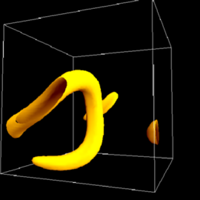
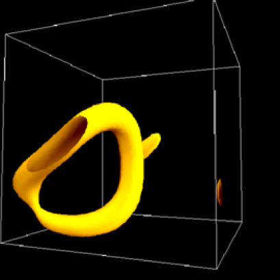
Figure 5: Loop formation from semilocal string segments. The figure shows two snapshots, at $t=70$ and $t=80$, of a $64^{3}$ numerical simulation of a network of semilocal strings with $\beta=0.05$ from Ref.[5], where the ends of an open segment of string join up to form a closed loop (see section 3.5 for a discussion of the simulations). Subsequently the loops seem to behave like those of topological cosmic string, contracting and disappearing.

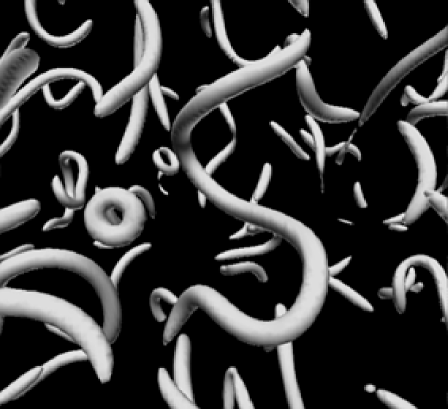
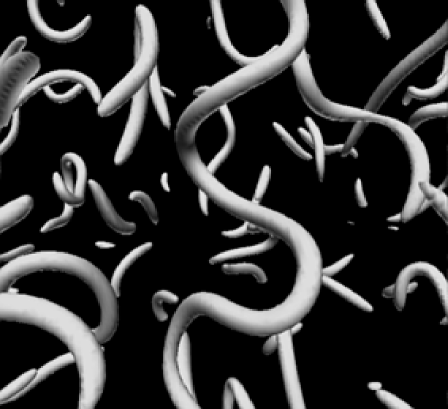
Figure 6: The growth of string segments to form longer strings. The figure shows two snapshots, at time $t=60$ and $t=70$ of a large $256^{3}$ numerical simulation of a network of semilocal strings with $\beta=0.05$ from Ref. [5]. Note several joinings of string segments, e.g. two separate joinings on the long central string, and the disappearance of some loops. The different apparent thickness of strings is entirely an effect of perspective. The simulation was performed on the Cray T3E at the National Energy Research Scientific Computing Center (NERSC). See section 3.5 for a discussion.

3.5 Numerical simulations of semilocal string networks

As the early Universe expanded and cooled to become what we know today it is very likely that it went through a number of phase transitions where topological (and possibly non-topological) defects are expected to have formed according to the Kibble mechanism [72, 135, 106]. Although the cosmological evidence for the existence of such defects remains unclear [10], there is plenty of experimental evidence from condensed matter systems that networks of defects do form in symmetry breaking phase transitions [95], the most recent confirmation coming from the Lancaster-Grenoble-Helsinki experiments in vortex formation in superfluid Helium [96]. An important question is whether semilocal (and electroweak) strings are stable enough to form in a phase transition.

We defer discussion of the electroweak case to section 9.4. Here we want to review recent numerical simulations of the formation and evolution of a network of $\beta<1$ semilocal strings [4, 5, 6] which show that such strings should indeed form in appreciable numbers in a phase transition. The results suggest that, even if no vortices are formed immediately after $\Phi$ has acquired a non-zero vacuum expectation value, the interaction between the gauge fields and the scalar fields is such that vortex formation does eventually occur simply because it is energetically favourable for the random distribution of magnetic fields present after the phase transition to become concentrated in regions where the Higgs field has a value close to that of the symmetric phase.

Even though they do not account for the expansion of the Universe, these simulations represent a first step towards understanding semilocal string formation in cosmological phase transitions and they have already provided very interesting insights into the dynamical evolution of such a network.

3.5.1 Description of the simulations

¿From a technical point of view, the numerical simulation of a network of semilocal strings has additional complications over that of $U(1)$ topological strings. Because there are not enough gauge degrees of freedom to cancel all of the scalar field gradients, the existence of string cores depends crucially on the way the fields (scalar and gauge) interact. Another problem, generic to all non-topological strings, is that the winding number is not well defined for configurations where the scalar is away from a maximal circle in the vacuum manifold, and this makes the identification of strings much more difficult than in the case of topological strings.

The strategy proposed in [4] to circumvent these problems is to follow the evolution of the gauge field strength in numerical simulations, since the field strength provides a gauge invariant indicator for the presence of vortices. The initial conditions are obtained by an extension of the Vachaspati-Vilenkin algorithm [125] appropriate to non-topological defects, plus a short period of dynamical evolution including a dissipation term (numerical viscosity) to aid the relaxation of configurations in the ‘basin of attraction’ of the semilocal string.

As with any new algorithm, it is essential to check that it reproduces previously known results accurately, and this has been done in [4]. Note that setting $\phi_{2}=0$ in the semilocal model obtains the Abelian Higgs model, thus comparison with topological strings is straightforward, and it is used repeatedly as a test case, both to check the simulation techniques and to minimise systematic errors when quoting formation rates. In particular, the proposed technique is tested in a two-dimensional toy model (representing parallel strings) in three different ways: a) restriction to the Abelian Higgs model gives good agreement with analytic and numerical estimates for cosmic strings in [125]; b) the results are robust under varying initial conditions and numerical viscosities (see Figure 8), and c) they are in good agreement with previous analytic and numerical estimates for semilocal string formation in [8, 57].

The results are summarized in Fig. 9. We refer the reader to refs. [4, 5, 6] for details; however, a few comments are needed to understand those figures.

$\bullet$ The study takes place in flat spacetime. Temporal gauge and rescaled units (32) are chosen. Gauss’ law, which here is a constraint derived from the gauge choice $Y_{0}=0$, is used to test the stability of the code.

$\bullet$ Space is discretized into a lattice with periodic boundary conditions. The equations of motion (56) are solved numerically using a standard staggered leapfrog method; however, to reduce its relaxation time an ad hoc dissipation term was added to each equation ($\eta\dot{\Phi}$ and $\eta\dot{Y}_{i}$ respectively). A range of strengths of dissipation was tested, and it did not significantly affect the number densities obtained. The simulations displayed in this section all have have $\eta=0.5$.

$\bullet$ The number density of defects is estimated by an extension of the Vachaspati-Vilenkin algorithm [125] by first generating a random initial configuration for the scalar fields drawn from the vacuum manifold, which is not discretised, and then finding the gauge field configuration that minimizes the energy associated with (covariant) gradients. If space is a grid of dimension $N^{3}$, the correlation length is chosen to be some number $p$ of grid points ($p=16$ in [4, 5]; the size of the lattice is either $N=64$ or $N=256$.) To obtain a reasonably smooth configuration for the scalar fields, one throws down random vacuum values on a $(N/p)^{3}$ subgrid; the scalar field is then interpolated onto the full grid by bisection. Strings are always identified with the location of magnetic flux tubes.

For cosmic strings, the two-dimensional toy model accurately reproduces the formation rates of [125]. For semilocal strings, on the other hand, the initial configurations generated in this way have a complicated flux structure with extrema of different values (top panel of Fig. 7), and it is far from clear which of these, if any, might evolve to form semilocal vortices; in order to resolve this ambiguity, the initial configurations are evolved forward in time. As anticipated, in the unstable regime $\beta>1$ the flux quickly dissipates leaving no strings. By contrast, in the stable regime $\beta<1$ stringlike features emerge when configurations in the “basin of attraction”of the semilocal string relax unambiguously into vortices (bottom panel of Fig. 7).

Since the initial conditions are somewhat artificial, the results were checked against various other choices of initial conditions, in particular different initial conditions for the gauge field and also thermal initial conditions for the scalar field (see Fig. 8). All the initial conditions in [4, 5] had zero initial velocities for the fields. Initial conditions with non-zero field momenta have not yet been investigated.

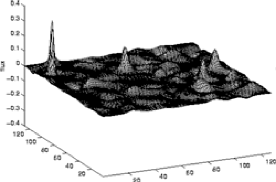
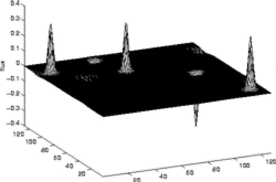
Figure 7: The flux tube structure in a two-dimensional semilocal string simulation with $\beta=0.05$, from Ref [4]. The upper panel ($t=0$) shows the initial condition after the process described in the text. The lower panel shows the configuration resolved into five flux tubes by a short period of dynamical evolution ($t=100$). These flux tubes are semilocal vortices.

3.5.2 Results and discussion

These simulations give very important information on the dynamics and evolution of a network of semilocal strings. In particular, they confirm our discussion in the previous subsection of the behaviour of the ends of string segments, and of strings with different colours. String segments are seen to grow in order to join nearby ones or form closed loops, and very short segments are also observed to collapse and disappear. The colour degrees of freedom do not seem to introduce any new forces between strings. Because the strings tend to grow or form closed loops, time evolution makes the network resemble more and more a network of topological strings (NO vortices) but with lower number densities

Note that the correlation length in the simulations is constrained to be larger than the size of the vortex cores, to avoid overlaps. This results in a minimal value of the parameter $\beta$ of around 0.05 (if $\beta$ is lowered further, the scalar string cores become too wide to fit into a correlation volume, in contradiction with the vacuum values assumed in a Vachaspati-Vilenkin algorithm). Figure 9 shows the results for seven different values of $\beta$ by taking several initial configurations on a $64^{3}$ grid smoothed over every $16$ grid-points. As expected, for $\beta<1$ the formation rate depends on $\beta$, tending to zero as $\beta$ tends to 1. The ratio of semilocal string density to cosmic string density in an Abelian Higgs model for the same value of $\beta$ is less than but of order one. For the lowest value of $\beta$ simulated ($\beta=0.05$), the semilocal string density is about one third of that of cosmic strings.

Figure 8: A test of the sensitivity of the results to the choice of initial conditions in a two-dimensional simulation with the algorithm proposed in section 3.5. The plot shows the number of semilocal strings formed per initial two-dimensional correlation volume. Each point is an average over ten simulations. Squares indicate that the vacuum initial conditions described in the text were used, while open circles indicate that non-vacuum (thermal) initial conditions were used. Both sets of initial conditions are seen to give comparable results. Statistical results are derived from a large suite of simulations (700 in all) carried out on a $64^{3}$ grid (from Ref. [4])

Figure 9: The ratio of lengths of semilocal and cosmic strings as a function of the stability parameter $\beta$, from [5].

One final word of caution about the possible cosmological implications of these simulations. We mentioned above that numerical viscosity was introduced to aid the relaxation of configurations close to the semilocal string. In an expanding Universe the expansion rate would provide some viscosity, though $\eta$ would typically not be constant. This may have an important effect on the production of strings. Indeed, note the different numbers of upward and downward pointing flux tubes in Fig. 7, despite the zero net flux boundary condition. The missing flux resides in the smaller ‘nodules’, made long-lived by the numerical viscosity; these are none other than the ‘skyrmions’ described in section 3. As was explained there, the natural tendency of skyrmions when $\beta<1$ is to collapse into strings, but the timescale for collapse increases quadratically with their size and Benson and Bucher [18] have argued that the effect of the expansion could stop the collapse of large skyrmions almost completely. On the other hand one expects skyrmions to be formed with all possible sizes, so the effect of the expansion on the number density of strings remains an open question. Another important issue that has not yet been addressed is whether these semilocal networks show scaling behaviour, and whether reconnections are as rare as the above simulations suggest. Both would have important implications for cosmology. However, the answer to these and other questions may have to wait until full numerical simulations are available.

3.6 Generalisations and final comments

i) Charged semilocal vortices

The semilocal string solution described earlier in this section is strongly static and z-independent, by which we mean that $D_{t}(\Phi)=D_{z}(\Phi)=0$. It is possible to relax these conditions while still keeping the Lagrangian and the energy independent of $z$ The idea is that, as we move along the $z$-direction, the fields move along the orbit of the global symmetries; in other words, Goldstone bosons are excited.

Abraham has shown that it is possible to construct semilocal vortices with finite energy per unit length carrying a global charge [2] in the Bogomolnyi limit $\beta=1$ . They satisfy a Bogomolnyi-type bound and are therefore stable. Perivolaropoulos [101] has constructed spinning vortices (however these have infinite energy per unit length).

ii) Semilocal models with $SU(N)_{\rm global}\times U(1)_{\rm local}$ symmetry

The generalization of semilocal strings to so-called Extended Abelian Higgs models with an N-component multiplet of scalars whose overall phase is gauged is straightforward [122, 56], and has been analysed in detail in [57, 49]. The strings are stable (unstable) for $\beta<1$ ($\beta>1$) and for $\beta=1$ they are degenerate in energy with skyrmionic configurations labelled by an $N-1$ complex vector. For winding $n$, and widely separated vortices, the $Nn$ complex parameters that characterize the configurations can be thought of as the $n$ positions in ${\rm I\!\!\,R}^{2}\sim{\rm I\!\!\!C}$ and the $(N-1)n$ ‘orientations’.

iii) Semilocal monopoles and generalized semilocality

We have seen that semilocal strings have very special properties arising from the fact that $\pi_{1}(G/H)=0$ but $\pi_{1}(G_{\rm local}/H_{\rm local})\neq 0$. An immediate question is whether it is possible to construct other non-topological defects such that

$$\pi_{k}(G/H)=0\qquad\qquad{\rm but}\qquad\qquad\pi_{k}(G_{\rm local}/H_{\rm local})\neq 0\ \ .$$ (81)

This possibility would be particularly interesting in the case of monopoles, $k=2$, since they might retain some of the features of global monopoles, in particular a higher annihilation rate in the early Universe. Surprisingly, the answer seems to be negative. Within a very natural set of assumptions, it was shown in [122] that the condition (81) can only be satisfied if the gauge group $G_{\rm local}$ is Abelian, and therefore one cannot have semilocal monopoles (nor any other defects satisfying conditions (81) with $k>1$).

However, Preskill has remarked that it is possible to define a wider concept of semilocality [103] by considering the larger approximate symmetry $G_{\rm approx}$ which is obtained in the limit where gauge couplings are set to zero. The symmetry $G_{\rm approx}$ is partially broken to the exact symmetry $G\sim G_{\rm local}\times G_{global}$ (modulo discrete transformations) when the gauge couplings are turned on It is then possible to have generalized semilocal monopoles associated with non-contractible spheres in $G_{\rm local}/H_{\rm local}$ which are contractible in the approximate vacuum manifold $G_{\rm approx}/H_{\rm approx}$ even though they are still non-contractible in the exact vacuum manifold $G/H$.

Another obvious possibility is to have topological monopoles with “colour”, by which we mean extra global degrees of freedom, if the symmetry $G\sim G_{\rm global}\times G_{\rm local}$ is such that the gauge orbits are non-contractible two-spheres, $\pi_{2}(G_{\rm local}/H_{\rm local})\neq 1$. Given that there are no semilocal monopoles [122], these monopoles must have $\pi_{2}(G/H)\neq 1$, so they are topologically stable, and they have additional global degrees of freedom.

iv) Semilocal defects and Hopf fibrations

In the semilocal model, the action of the gauge group fibres the vacuum manifold $S^{3}$ as a non-trivial bundle over $S^{2}\sim{\rm I\!\!\!C}P^{1}$, the Hopf bundle. The fact that this bundle is non-trivial is at the root of conditions (61), and is ultimately the reason why the topological criterion for the existence of strings fails. In view of this, Hindmarsh [57] has proposed an alternative definition of a semilocal defect: it is a defect in a theory whose vacuum manifold is a non-trivial bundle with fibre $G_{\rm local}/H_{\rm local}$.

Extended Abelian Higgs models [57] are similarly related to the fibrations of the odd-dimensional spheres $S^{2N-1}$ with fibre $S^{1}$ and base space ${\rm I\!\!\!C}P^{N-1}$. A natural question to ask is if the remaining Hopf fibrations of spheres can also be realised in a field theoretic model. This question was answered affirmatively in [58] for the $S^{7}\ {S^{3}\atop\rightarrow}\ S^{4}$ fibration in a quaternionic model. Other non-trivial bundles were also implemented in this paper, but to date the field theory realisation of the $S^{15}\ {S^{7}\atop\rightarrow}\ S^{8}$ Hopf bundle remains an open problem.

v) Monopoles and textures in the semilocal model:

Since the gauge field is Abelian, ${\rm div}\vec{B}=0$, and isolated magnetic monopoles are necessarily singular in semilocal models. The only way to make the singularity disappear is by embedding the theory in a larger non-Abelian theory which provides a regular core, or by putting the singularity behind an event horizon [49]. One important question that has not yet been addressed is if the scalar gradients in these spherical monopoles make them unstable to angular collapse into a flux tube. A related system where this happens is in $O(3)$ global monopoles where the spherically symmetric configuration is unstable. In the semilocal case, it is possible that the pressure from the magnetic field might prevent the instability towards angular collapse.

Finally, note that, because $\pi_{3}(S^{3})={\rm\angle\!\!\!Z}$, there is also the possibility of textures in the semilocal model (51). In contrast with purely scalar $O(4)$ models, their collapse seems to be stopped by the pressure from the magnetic field [57]. Of course they can still unwind by tunnelling.

vi) We should point out that systems related to the semilocal model have been studied in condensed matter. In [26], the system was an unconventional superconductor where the role of the global SU(2) group was played by the spin rotation group. In [129] the hypothetical case of an “electrically charged” A-phase of ${}^{3}\rm He$, i.e. a superconductor with the properties of ${}^{3}\rm He$-A, was considered (see section 11.1 for a brief discussion of the A and B phases of ${}^{3}\rm He$). In this case the global group was SO(3), the group of orbital rotations. Both papers discussed continuous vortices in such superconductors, which correspond to the “skyrmions” discussed here.

4 Electroweak strings

In this section we introduce electroweak strings. There are two kinds: one, more precisely known as the Z-string, carries Z-magnetic flux, and is the type that was discussed by Nambu and that becomes stable as it approaches the semilocal limit. It is associated with the subgroup generated by

$$T_{Z}=n^{a}T^{a}-\sin^{2}\theta_{w}Q\ .$$

There are other strings in the GSW model that carry $SU(2)$ magnetic flux, called $W$-strings. There is a one-parameter family of W strings which are all gauge equivalent to one another, and they are all unstable. They are generated by a linear combination of the SU(2) generators $T^{+}$ and $T^{-}$. These will be discussed in more detail in the next section.

4.1 The Z string

Modulo gauge transformations, the configuration describing a straight, infinitely long Z-string along the $z$-axis is [118]:

 

$${\Phi}$$

  (82)

where $f$ and $v$ are the Nielsen-Olesen profiles that solve the equations (40). It is straightforward to show that this is a solution of the bosonic equations of motion (alternatively, one can show that it is an extremum of the energy [118]). Equations (82) describe a string with unit winding. The solutions with higher winding number can be constructed in an analogous way, but note that the winding number is not a topological invariant. The unstable string can decay by unwinding until it reaches the vacuum sector.

The solution (82) reduces to the semilocal string in the limit $\sin^{2}\theta_{w}=1$, and therefore it is classically stable for $\beta<1$ and unstable for $\beta>1$ (see section 7), where $\beta$ is now the ratio between the Higgs mass, $\sqrt{2}\lambda\eta$ and the Z-boson mass $g_{z}\eta/2$, thus

$$\beta={8\lambda\over g_{z}^{2}}$$ (83)

The Z-string configuration is axially symmetric, as it is invariant under the action of the generalised angular momentum operator

$$M_{z}=L_{z}+S_{z}+I_{z}$$ (84)

where $L_{z}$, $S_{z}$ and $I_{z}$ are the orbital, spin and isospin parts, respectively, defined in section 9.1.

The Z-string carries a Z-magnetic flux

$$F_{Z}={4\pi\over g_{z}}$$ (85)

thus particles whose Z charge is not an integer multiple of $g_{z}/2$ will have Aharonov-Bohm interactions with the string (see section 8.3). The Z-string can terminate on magnetic monopoles (such configurations are discussed in section 5). When a string terminates, the discrete Aharonov-Bohm interaction can be smoothly deformed to the trivial interaction. The smoothness is provided by the presence of the magnetic flux of the monopole.

$\bullet$ Note that, in the background given by (82), the covariant derivative becomes

$${\bf d}_{\mu}\equiv D_{\mu}|_{\rm Z-string}=\partial_{\mu}+i{g_{z}\over 2}\left[-2(T^{3}-Q\sin^{2}\theta_{w})\right]Z_{\mu}$$ (86)

in particular, left and right fermion fields couple to $Z_{\mu}$ with different strengths, since the effective Z-charge

$${\bf q}=-2(T^{3}-Q\sin^{2}\theta_{w})$$ (87)

has different values, $q_{R}=q_{L}\pm 1$. (Note that $\bf q$ is proportional to the string generator $T_{z}$, defined in equation (17). The proportionality factor has been introduced for later convenience). This will be important in section 8.3. Note also that, for the Higgs field,

$${\bf q}={\rm diag}(-\cos 2\theta_{w},1)$$ (88)

$\bullet$ Ambjørn and Olesen [11] and, more recently, Bimonte and Lozano [21] have derived Bogomolnyi-type bounds for periodic configurations in the GSW model. They consider static configurations such that physical observables are periodic in the $xy$-plane and cylindrically symmetric in each cell. If $A$ is the area of the basic cell, they find that the energy (per unit length) satisfies

$$\cases{{E}\geq({1/2e^{2}})m_{W}^{2}(2g^{\prime}F_{Y}-m_{W}^{2}A)&if $m_{H}\geq m_{Z}$\cr&\cr{E}\geq({1/2e^{2}})({m_{W}m_{H}/m_{Z}})^{2}(2g^{\prime}F_{Y}-m_{W}^{2}A)&if $m_{H}<m_{Z}$\cr}$$ (89)

where $F_{Y}$ is the magnetic flux of the hypercharge field through the cell. Note that the top line of (89) reduces to the familiar $E\geq\langle\Phi^{\dagger}\Phi\rangle qF_{Y}$ for the Abelian Higgs and semilocal case in the $g\to 0$ limit (with $q=g^{\prime}/2$). In the non-Abelian case the bound involves an area term and therefore does not admit a topological interpretation.

In the Bogomolnyi limit, $m_{H}=m_{Z}$, the bound is saturated for configurations satisfying the first order Bogomolnyi equations

 

$${D_{1}+iD_{2}\Phi}$$

  (90)

A solution to these equations describing a lattice of Z-strings was constructed in [21]. Other periodic configurations with symmetry restoration had been previously found in the presence of an external magnetic field in [11].

5 The zoo of electroweak defects

The electroweak Z-string is one member in the zoo of electroweak defects. Other members include the electroweak monopole, dyon and the W-string. The latter fall in the class of “embedded defects” and this viewpoint provides a simple way to characterize them. The electroweak sphaleron is also related to the electroweak defects.

5.1 Electroweak monopoles

To understand the existence of magnetic monopoles in the GSW model, recall the following sequence of facts:

• The Z-string does not have a topological origin and hence it is possible for it to terminate.

• As the hypercharge component of the Z-field in the string is divergenceless it cannot terminate. Therefore it must continue from within the string to beyond the terminus.

• However, beyond the terminus, the Higgs is in its vacuum and the hypercharge magnetic field is massive. Then, if the massive hypercharge flux was to continue beyond the string, it would cost an infinite amount of energy and this is not possible.

• The only means by which the hypercharge field can continue beyond the terminus is in combination with the SU(2) fields such that it forms the massless electromagnetic magnetic field.

So the terminus of the Z-string is the location of a source of electromagnetic magnetic field, that is, a magnetic monopole [94]. We now make this argument more quantitative.

Assume that we have a semi-infinite Z-string along the $-z$ axis with terminus at the origin (see Fig. 10). Let us denote the A- and Z- magnetic fluxes through a spatial surface by $F_{A}$ and $F_{Z}$. These are given in terms of the W- and Y- fluxes by taking surface integrals of the field strengths (see eqs. (19), (20)). Therefore

$$F_{Z}=\cos\theta_{w}F_{n}-\sin\theta_{w}F_{Y}\ ,\ \ \ \ F_{A}=\sin\theta_{w}F_{n}+\cos\theta_{w}F_{Y}\ ,$$ (91)

where we have denoted the SU(2) flux (parallel to $n^{a}$ in group space) by $F_{n}$ and the hypercharge flux by $F_{Y}$.

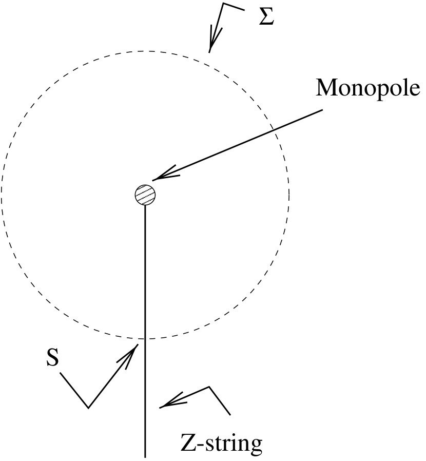
Figure 10: The outgoing hypercharge flux of the monopole passing through the surface ${\Sigma-S}$ should equal the incoming hypercharge flux through the Z-string.

Now consider a large sphere $\Sigma$ centered on the string terminus. The field configuration is such that there is only A-flux through $\Sigma$ except near the South pole ($S$) of $\Sigma$, where there is only a $Z$ magnetic flux. Hence,

$$F_{Z}|_{\Sigma-S}=0\ ,\ \ F_{A}|_{S}=0\ .$$ (92)

Together with (91) this gives,

$$F_{n}|_{\Sigma-S}=\tan\theta_{w}F_{Y}|_{\Sigma-S}\ ,\ \ \ F_{n}|_{S}=-\cot\theta_{w}F_{Y}|_{S}\ .$$ (93)

The hypercharge flux must be conserved as it is divergenceless. So

$$F_{Y}|_{\Sigma-S}=-F_{Y}|_{S}\equiv F_{Y}\ ,$$ (94)

and, inserting this and (93) in (91) yields

$$F_{A}|_{\Sigma-S}={{F_{Y}}\over{\cos\theta_{w}}}\ ,\ \ \ F_{Z}|_{S}={{F_{Y}}\over{\sin\theta_{w}}}\ .$$ (95)

Now the flux in the $Z-$string along the $-z$ axis is quantized in units of $4\pi/g_{z}$ (recall $g_{z}=e/\cos\theta_{w}\sin\theta_{w}$ gives the coupling of the Z boson to the Higgs field). Therefore, for the unit winding string,

$$F_{Z}|_{S}={{4\pi}\over{g_{z}}}\ .$$ (96)

Then (95) yields,

$$F_{Y}={{4\pi}\over{g_{z}}}\sin\theta_{w}\ ,\ \ \ F_{A}|_{\Sigma-S}={{4\pi}\over{g_{z}}}\tan\theta_{w}={{4\pi}\over{e}}\sin^{2}\theta_{w}\$$ (97)

Hence the terminus of the string has net A-flux emanating from it and hence it is a magnetic monopole.

The electromagnetic flux of the electroweak monopole appears to violate the Dirac quantization condition. However this is not true since one must also take the Z-string into account when deriving the quantization condition relevant to the electroweak monopole This becomes clearer when we work out the magnetic flux for the $SU(2)$ fields. Using (93) with (97), the net non-Abelian flux is:

$$F_{n}=F_{n}|_{S}+F_{n}|_{\Sigma-S}={{4\pi}\over{g}}$$ (98)

just as we would expect for a ’t Hooft-Polyakov monopole [62]. That is, the Dirac quantization condition works perfectly well for the SU(2) field and the monopole charge is quantized in units of $4\pi/g$. Another way of looking at (98) is to say that the electroweak monopole is a genuine SU(2) monopole in which there is a net emanating $U(1)_{n}\subset SU(2)$ flux. The structure of the theory, however, only permits a linear combination of this flux and hypercharge flux to be long range and so there is a string attached to the monopole. But this string is made of Z field which is orthogonal to the electromagnetic field and so the string does not surreptitiously return the monopole electromagnetic flux. Also, the magnetic charge on the monopole is conserved and electroweak monopoles can only disappear by annihilating with antimonopoles.

It is useful to have an explicit expression describing the asymptotic field of the electroweak monopole and string. Nambu’s monopole-string configuration, denoted by $({\bar{\Phi}},{\bar{W}}_{\mu}^{a},{\bar{Y}}_{\mu})$, is

$${\bar{\Phi}}={{\eta}\over{\sqrt{2}}}\pmatrix{\cos(\theta/2)\cr\sin(\theta/2)e^{i\varphi}}\$$ (99)

where, $\theta$ and $\varphi$ are spherical coordinates centred on the monopole, and the gauge field configuration is,

$$g{\bar{W}}_{\mu}^{a}=-\epsilon^{abc}n^{b}\partial_{\mu}n^{c}+i\cos^{2}\theta_{w}n^{a}({\bar{\Phi}}^{{\dagger}}~{}\partial_{\mu}{\bar{\Phi}}-\partial_{\mu}{\bar{\Phi}}^{{\dagger}}~{}{\bar{\Phi}})$$ (100)

$$g^{\prime}{\bar{Y}}_{\mu}=-i\sin^{2}\theta_{w}({\bar{\Phi}}^{{\dagger}}~{}\partial_{\mu}{\bar{\Phi}}-\partial_{\mu}{\bar{\Phi}}^{{\dagger}}~{}{\bar{\Phi}})\$$ (101)

where, $n^{a}$ is given in eq. (16).

Note that there is no electroweak configuration that represents a magnetic monopole surrounded by vacuum.

5.2 Electroweak dyons

Given that the electroweak monopole exists, it is natural to ask if dyonic configurations exist as well. We now write down dyonic configurations that solve the asymptotic field equations [121]. The existence of such configurations is implicit in Nambu’s original paper in the guise of what he called “external” potentials [94]. Essentially, the dyon solution is an electroweak monopole together with a particular external potential.

The ansatz that describes an electroweak dyon connected by a semi-infinite $Z$ string is:

$$\Phi={\bar{\Phi}}$$ (102)

$$W^{a}={\bar{W}}^{a}-dt{{n^{a}{\dot{\zeta}}}\over\cos\theta_{w}}$$ (103)

$$Y={\bar{Y}}-dt{{\dot{\zeta}}\over\sin\theta_{w}}$$ (104)

where, $\zeta=\zeta(t,\vec{x})$, overdots denote partial time derivatives and barred fields have been defined in the previous subsection.

We now need to insert this ansatz into the field equations and to find the equation satisfied by $\zeta$. Some algebra leads to

$$\partial^{i}\partial_{i}{\dot{\zeta}}=0\ ,\ \ \ \partial_{t}\partial^{i}{\dot{\zeta}}=0$$ (105)

which can be solved by separating variables,

$$\zeta=\xi(t)f(\vec{x})\ .$$ (106)

This leads to

$${\ddot{\xi}}=0\ ,\ \ \ \nabla^{2}f=0\ .$$ (107)

The particular solution that we will be interested in is the solution that gives a dyon. Hence, we take:

$$\xi=\xi_{0}t\ ,\ \ \ f(r)=-{{q\sin\theta_{w}\cos\theta_{w}}\over{4\pi\xi_{0}}}{1\over r}\ ,$$ (108)

where, $\xi_{0}$ and $q$ are constants. Now, using (108), together with (103), (104) and (106), we get the dyon electric field:

$${\vec{E}}_{A}={q\over{4\pi}}{{\vec{r}}\over{r^{3}}}\ .$$ (109)

For a long segment of string, the monopole and the antimonopole at the ends are well separated and we can repeat the above analysis for both of them independently. Therefore, the electric charge on the antimonopole at one end of a Z-string segment is uncorrelated with the charge on the monopole at the other end of the string. This means that we can have dyons of arbitrary electric charge at either end of the string. The situation will change with the inclusion of fermions since these can carry currents along the string and transport charge from monopole to antimonopole.

This completes our construction of the dyon-string system in the GSW model. As of now, the charge $q$ on the dyon is arbitrary. Quantum mechanics implies that the electric charge must be quantized. If we include a $\theta$ term in the electroweak action (but no fermions):

$$S_{\theta}={{g^{2}\theta}\over{32\pi^{2}}}\int d^{4}xW_{\mu\nu}^{a}{\tilde{W}}^{\mu\nu^{a}}\$$ (110)

where

$${\tilde{W}}^{\mu\nu^{a}}={1\over 2}\epsilon^{\mu\nu\lambda\sigma}W_{\mu\nu}^{a}\ ,$$ (111)

then the charge quantization condition becomes

$$q=\left(n+{\theta\over{2\pi}}\right)e\ .$$ (112)

This agrees with the standard result for dyons [134].

In the GSW model with fermions, it is known that the $\theta$ term can be eliminated by a rotation of the fermionic fields. This argument can be turned around to argue that the CP violation in the mass matrix of the fermions will lead to an effective $\theta$ term and so the electroweak monopoles will indeed have a fractional charge with $\theta$ being related to the CP violation in the mass matrix. The precise value of the fractional electric charge on electroweak monopoles has not yet been calculated and remains an open problem.

It should be mentioned that, even though the electric charge on an electroweak dyon can be fractional as in (112), the total electric charge on the dyon-string system is always integral because the CP violating fractional charge on the monopole is equal and opposite to that on the antimonopole.

5.3 Embedded defects and W-strings:

A very simple way of understanding the existence of electroweak string solutions is in terms of embedded defects. While this method does not shed any light on the stability of the electroweak string, it does provide a scheme for finding other solutions.

The idea is that the electroweak symmetry group contains several $U(1)$ subgroups which break completely when the electroweak symmetry breaks. Corresponding to each such breaking, one might have a string solution. A more complete analysis tells us when such a solution can exist [123, 15, 34, 80].

Consider the general symmetry breaking

$$G\rightarrow H$$ (113)

Suppose $G_{emb}$ is a subgroup of $G$ which, in this process, breaks down to $G_{emb}\cap H$. Then we ask the question: when are topological defects in the symmetry breaking

$$G_{emb}\rightarrow G_{emb}\cap H$$ (114)

also solutions in the full theory? An answer to this question requires separating the gauge fields into those that transform within the $G_{emb}$ subgroup and those that do not. Similarly, the Higgs field components are separated into those that lie in the embedded vector space of scalar fields and those that do not. Then, it is possible to write down general conditions under which solutions can be embedded [15, 34]. Here we shall not describe these conditions but remark that the Z-string is due to the embedded symmetry breaking

$$U(1)_{Z}\rightarrow 1$$ (115)

where the $U(1)_{Z}$ is generated by $T_{Z}$, defined in eq. (17). Now, there are other $U(1)$’s that can be embedded in the GSW model which lie entirely in the $SU(2)$ factor. For example, we can choose $U(1)_{1}$ which is generated by $T^{1}$ (one of the off-diagonal generators of $SU(2)$). Since we have

$$U(1)_{1}\rightarrow 1$$ (116)

when the electroweak symmetry breaks, there is the possibility of another string solution in the GSW model. Indeed, it is easily checked that this string can be embedded in the GSW model and the solution is called a W-string. By considering a one parameter family of $U(1)$ subgroups generated by

$$T_{\zeta}=\cos(\zeta)~{}T^{1}+\sin(\zeta)~{}T^{2}$$ (117)

we can generate a one parameter family of W-strings

$$\Phi={\eta\over{\sqrt{2}}}f_{NO}(\rho)\pmatrix{\cos\varphi\cr ie^{-i\zeta}\sin\varphi}$$ (118)

$$W^{1}=-{2\over g}\cos\zeta~{}{v_{NO}(\rho)}d\varphi~{},\ \ W^{2}=-{2\over g}\sin\zeta~{}{v_{NO}(\rho)}d\varphi~{},$$ (119)

and all other fields vanish. Although the string solutions are gauge equivalent for different values of $\zeta$, the parameter does take on physical meaning when considering multi-string configurations in which the value of $\zeta$ is different for different strings [15].

Note that the generator (117) can be obtained from $T^{1}$ by the action of the unbroken (electromagnetic) group,

$$T_{\zeta}=e^{i\zeta Q}T^{1}e^{-i\zeta Q}$$ (120)

With this in mind, Lepora et al [80, 81] have classified embedded vortices. The idea is that, for a general symmetry breaking $G\to H$,the Lie algebra of $G$, $\cal G$, decomposes naturally into a direct sum of the space $\cal H$ of generators of the unbroken subgroup $H$ (the ones associated with massless gauge bosons) and the space $\cal M$ of generators associated with massive gauge bosons: ${\cal G}={\cal H}+{\cal M}$. The action of $H$ on the subspace $\cal M$ further decomposes $\cal M$ into irreducible subspaces. The classification of embedded vortices is based on this decomposition, as we now explain.

Recall (eq. 37) that finite energy vortices are associated with gauge orbits on the vacuum manifold. Choosing a base point $\Phi_{0}$ in the vacuum manifold, each embedded vortex can be associated to a Lie algebra generator which is tangent to the gauge orbit describing the asymptotic scalar field configuration of the vortex. The unbroken subgroup $H$ at $\Phi_{0}$ “rotates” the various gauge orbits among themselves as in eq. (120). Thus, the action of $H$ splits the space of gauge orbits into irreducible subspaces.

Except for critical values of the coupling constants (which could lead to so-called combination vortices), it can be shown [15, 80] that embedded vortices have to lie entirely in one of these irreducible subspaces. If the subspaces have dimension greater than one, then there may be a family of gauge equivalent vortices.

In the GSW model, for instance, the Lie Algebra decomposes into ${\cal H}+{\cal M}_{1}+{\cal M}_{2}\$ where $\cal H$ is spanned by the charge $Q$, ${\cal M}_{1}$ is a one-dimensional subspace spanned by $T_{Z}$ (corresponding to the Z-string) and ${\cal M}_{2}$ is a two-dimensional subspace comprising all W-string generators $T_{\zeta}$.

Both the W- and the Z-string are embedded string solutions in the GSW model. What makes the Z-string more interesting is its unexpected stability properties. It can be shown [80] that only those vortices lying in one-dimensional subspaces can have a stable semilocal limit. Thus, embedded vortices belonging to a family are always unstable.

Another important difference is that the Z-string is known to terminate on magnetic monopoles but this is not true of the W-string. The W-string can terminate without any emanating electromagnetic fields since it is entirely within the $SU(2)$ sector of the GSW model.

It is straightforward to embed domain walls in the GSW model. There are no embedded monopoles in the GSW model since there is no SU(2) subgroup that is broken to U(1).

6 Electroweak strings in extensions of the GSW model

Electroweak strings have been discussed in various extensions of the GSW model. We describe some of this work below. We do not, however, discuss extensions in which topological strings are produced at the electroweak scale [36, 22].

6.1 Two Higgs model

As discussed in Sec. 5.3, the Z-string is an embedded string in the GSW model. The general conditions that enable the embedding are valid even with a more complicated Higgs structure. Here we will consider the two Higgs doublet model which is inspired by supersymmetric extensions of the GSW model.

In a two Higgs doublet model, the Higgs structure of the GSW model is doubled so that we have scalars $\Phi_{1}$ and $\Phi_{2}$ and the scalar potential is [69]

$$V(\Phi_{1},\Phi_{2}) = \lambda_{1}(\Phi_{1}^{\dagger}\Phi_{1}-\frac{\nu_{1}^{2}}{2})^{2}+\lambda_{2}(\Phi_{2}^{\dagger}\Phi_{2}-\frac{\nu_{2}^{2}}{2})^{2}+\lambda_{3}[(\Phi_{1}^{\dagger}\Phi_{1}-\frac{\nu_{1}^{2}}{2})+(\Phi_{2}^{\dagger}\Phi_{2}-\frac{\nu_{2}^{2}}{2})]^{2}$$ (121)

$$+ \lambda_{4}[(\Phi_{1}^{\dagger}\Phi_{1})(\Phi_{2}^{\dagger}\Phi_{2})-(\Phi_{1}^{\dagger}\Phi_{2})(\Phi_{2}^{\dagger}\Phi_{1})]+\lambda_{5}[{\rm Re}(\Phi_{1}^{\dagger}\Phi_{2})-\frac{\nu_{1}\nu_{2}}{2}\cos\xi]^{2}$$

$$+ \lambda_{6}[{\rm Im}(\Phi_{1}^{\dagger}\Phi_{2})-\frac{\nu_{1}\nu_{2}}{2}\sin\xi]^{2}\$$

$$+ \lambda_{7}[{\rm Re}(\Phi_{1}^{\dagger}\Phi_{2})-\frac{\nu_{1}\nu_{2}}{2}\cos\xi]~{}[{\rm Im}(\Phi_{1}^{\dagger}\Phi_{2})-\frac{\nu_{1}\nu_{2}}{2}\sin\xi]\ \ .$$

Here $\nu_{1}$ and $\nu_{2}$ are the respective VEVs of the two doublets, $\lambda_{i}$ are coupling constants and the parameter $\xi$ is a phase

In polar coordinates, the solution for the two Higgs Z-string is:

$$\Phi_{1}=\nu_{1}f_{1}(\rho)e^{i\varphi}\pmatrix{0\cr 1\cr}$$ (122)

$$\Phi_{2}=\nu_{2}f_{2}(\rho)e^{i\varphi}\pmatrix{0\cr 1\cr}$$ (123)

$${\vec{Z}}=-{2\over{g_{z}}}{{v(\rho)}\over{\rho}}{\hat{\varphi}}$$ (124)

with the profile functions satisfying differential equations similar to the Abelian-Higgs case. These have been studied in Ref. [37] where the stability has also been analyzed (also see [115]).

6.2 Adjoint Higgs model

The GSW model with an additional $SU(2)$ field in the adjoint representation, $\vec{\chi}$, is what we shall refer to as the “adjoint Higgs model”. The impact of the adjoint field on electroweak defects was considered in Ref. [71].

The bosonic sector of the adjoint Higgs model is:

$$L=T_{ew}+|(\partial_{\mu}+ig\epsilon^{a}W_{\mu}^{a}){\vec{\chi}}|^{2}-V(\Phi,{\vec{\chi}})+L_{f}\$$ (125)

where, $T_{ew}$ is the gradient part of the bosonic sector of the electroweak Lagrangian, $L_{f}$ is the fermionic part of the Lagrangian, $\epsilon^{a}_{ij}=\epsilon_{aij}$ ($a,i,j=1,2,3$) and,

$$V(\Phi,{\vec{\chi}})=-\mu_{2}^{2}\Phi^{{\dagger}}\Phi-\mu_{3}^{2}{\vec{\chi}}^{2}+\lambda_{2}(\Phi^{{\dagger}}\Phi)^{2}+\lambda_{3}{\vec{\chi}}^{4}+a{\vec{\chi}}^{2}\Phi^{{\dagger}}\Phi+b{\vec{\chi}}\cdot\Phi^{{\dagger}}{\vec{\tau}}\Phi\;.$$ (126)

If we impose an additional $Z_{2}$ symmetry on the Lagrangian under $\Phi\rightarrow+\Phi\ ,\ \ \ {\vec{\chi}}\rightarrow-{\vec{\chi}}\ .$ the symmetry is $([SU(2)_{L}\times U(1)_{Y}]/Z_{2})\times Z_{2}$ and we must set $b=0$. In what follows, we shall only consider this case and henceforth ignore the last (cubic) term in the potential. In this case, an additional simplification is that the leptons and quarks do not couple to $\vec{\chi}$ and so $L_{f}$ is identical to the fermionic Lagrangian of the GSW model. (If the $Z_{2}$ symmetry is absent, the cubic term in the potential is allowed but is constrained to be small by experiment.)

In a cosmological context, as the universe cools down from high temperatures, if the parameters lie in a certain range [71] there will first be a phase transition in which the adjoint field gets a VEV. The VEV of the adjoint will break the $SU(2)$ factor of the high temperature symmetry group to $U(1)$. If the VEV of ${\vec{\chi}}$ is along the $(0,0,1)$ direction, the generator of this $U(1)$ will be $T^{3}$ and we will denote the unbroken subgroup as $U(1)_{3}$. So the symmetry breaking pattern at this stage is

$$([SU(2)\times U(1)_{Y}]/Z_{2})\times Z_{2}\rightarrow([U(1)_{3}\times U(1)_{Y}]/Z_{2})\times Z_{2}$$ (127)

and topological magnetic monopoles will be produced with pure $U(1)_{3}$ flux

At a lower temperature, the doublet field will also get a VEV with the effect,

$$([U(1)_{3}\times U(1)_{Y}]/Z_{2})\times Z_{2}\rightarrow U(1)_{em}\ .$$ (128)

where, as usual, the electromagnetic charge operator is

$$Q=T^{3}+{Y\over 2}$$ (129)

The electromagnetic component (A) from the monopoles is massless but the orthogonal part (Z) of the flux is massive and gets confined to a string. This is the Z-string. In addition, the breaking of the $Z_{2}$ factor gives domain walls.

In the second stage of symmetry breaking, the Z-string is topological and hence is stable. The presence of magnetic monopoles from the earlier symmetry breaking means that the Z-strings can break by terminating on monopoles. But, as the monopoles form at a higher energy scale, their mass is much larger than the energy scale at which strings form and which sets the scale for the tension in the string. So the string can only break by instanton processes.

At a yet lower temperature, the VEV of the adjoint turns off. This makes no difference to the symmetry structure of the model (apart from restoring the $Z_{2}$ symmetry and eliminating the domain walls) and hence no significant difference to the monopoles connected by strings. However, it does affect the stability of the strings since the monopoles are no longer topological.

7 Stability of electroweak strings

7.1 Heuristic stability analysis

As described in [118], the Z-string goes over into the semilocal string in the limit $\theta_{w}\rightarrow\pi/2$ and hence the stability of the Z-string should match on continuously to that of the semilocal string. Therefore we expect that Z-strings should be stable if $\theta_{w}$ is close to $\pi/2$ and $m_{H}\leq m_{Z}$.

The stability analysis to certain subsets of perturbations can be carried out much more easily than to the completely general perturbations. The subset includes perturbations in the Higgs field and W-fields separately. Such analyses may be found in [118, 119, 15] and [99].

(i) Higgs field perturbations: Perturbations in the Higgs field alone have maximum destabilizing effect for $\theta_{w}=\pi/4$ [15] and, in this case, it is easy to see that the Z-string is unstable. Consider the one parameter family of field configurations

$$\Phi(\vec{x};\xi)=\cos\xi~{}\Phi_{0}(\cos\xi~{}{\vec{x}})+\sin\xi~{}\Phi_{\perp}$$ (130)

$$Z_{j}(\vec{x};\xi)=\cos\xi~{}Z_{(0)j}(\cos\xi~{}\vec{x})$$ (131)

where, the string solution is denoted by the $0$ subscript, $\xi\in[0,\pi/2]$ and

$$\Phi_{\perp}={\eta\over{\sqrt{2}}}\pmatrix{1\cr 0\cr}\ .$$ (132)

For $\xi=0$ the field configuration is the unperturbed Z-string while for $\xi=\pi/2$ it is the vacuum. The energy per unit length of this field configuration can be evaluated and is found to be:

$$E(\xi)=\cos^{2}\xi~{}E(\xi=0)\ .$$ (133)

Hence the energy per unit length of the string is a monotonically decreasing function of $\xi$ and so the string is unstable to decay into the vacuum.

(ii) Incontractible two spheres: James [66], and, Klinkhamer and Olesen [75] have constructed the Z- and W-string solutions by considering incontractible two spheres in the space of electroweak field configurations in two spatial dimensions. The idea was introduced by Taubes [114] and was used by Manton to construct the sphaleron [90, 74]. The procedure (known as the “minimax” procedure) is to construct a set of field configurations that are labelled by some parameters $\mu_{i}$. If this set is incontractible in the space of field configurations, then there exist (subject to certain assumptions [90]) values of the parameters for which the field configuration extremizes the energy functional. For example, Klinkhamer and Olesen [75] give the following construction for the Z-string in terms of a two parameter ($\mu,\nu$) family of field configurations

$$\pi/2\leq[\mu\nu]\leq\pi\,: W=0\ ,\ \ \ Y=0$$ (134)

$$\Phi=(1-\{1-h(\rho)\}\sin[\mu\nu]){\eta\over{\sqrt{2}}}\pmatrix{0\cr 1\cr}$$

$$0\leq[\mu\nu]\leq\pi/2\,: W=-f(\rho)G^{a}T^{a}\ ,\ \ \ Y=f(\rho)\sin^{2}\theta_{w}F^{3}$$ (135)

$$\Phi=h(\rho){\eta\over{\sqrt{2}}}\Omega U\pmatrix{0\cr 1\cr}$$

where, $W$ and $Y$ are Lie algebra valued 1-forms (e.g. $W=W_{\mu}^{a}T^{a}dx^{\mu}$), $[\mu\nu]\equiv{\rm max}(|\mu|,|\nu|)$,

$$F^{a}T^{a}=2iU^{-1}dU\ ,$$ (136)

$$G^{a}T^{a}=\Omega U[F^{1}T^{1}+F^{2}T^{2}+\cos^{2}\theta_{w}F^{3}T^{3}]U^{-1}\Omega^{-1}\ ,$$ (137)

$$U(\mu,\nu,\varphi)=-i\sin\mu\tau_{1}-i\cos\mu\sin\nu\tau_{2}-i\cos\mu\cos\nu\sin\varphi\tau_{3}+\cos\mu\cos\nu\cos\varphi{\bf 1}\ ,$$ (138)

$$\Omega=U(\mu,\nu,\varphi=0)^{-1}\ ,$$ (139)

and the functions $f(\rho)$ and $h(\rho)$ satisfy the boundary conditions

$$f(0)=0=h(0)\ ,\ \ \ f(\infty)=1=h(\infty)\ .$$ (140)

This set of field configurations labelled by the parameters $\mu,\nu\in[-\pi,\pi]$ defines an incontractible two sphere in the space of field configurations. This is seen by considering the fields as if they were defined on the three-sphere on which the coordinates are $\varphi$, $\mu$ and $\nu$ and then showing that the field configurations define a topologically non-trivial mapping from this $S^{3}$ to the vacuum manifold which is also an $S^{3}$. Then the minimax procedure says that there is an extremum of the energy at some value of the parameters. By inserting the field configurations into the energy functional, it can be checked that the extremum occurs at $\mu=0=\nu$, when the configuration coincides with that of the Z-string. Furthermore, for $\theta_{w}\leq\pi/4$, the extremum is a maximum and hence the Z-string is unstable.

A very similar analysis has been done [66, 75] for the W-string confirming the result [15] that it is always unstable.

(iii) W-condensation: There is also a well-known [12] instability to perturbations in the W-fields alone called “W-condensation”. Application of this instability to the Z-string may be found in [99, 119, 120, 7]. A heuristic argument goes as follows.

The energy of a mass $m$, charge $e$ and spin $s$ particle in a uniform magnetic field $\vec{B}$ along the z-axis is given by:

$$E^{2}=p_{z}^{2}+m^{2}+(2n+1)eB-2e{\vec{B}}\cdot{\vec{s}}$$ (141)

where $n=0,1,2,...$ labels the Landau levels and $p_{z}$ is the momentum along the z-axis. Now, if $s=1$, the right-hand side can be negative for $p_{z}=0$, $n=0$ provided

$$B>{{m^{2}}\over e}~{}.$$ (142)

This signals an instability towards the spontaneous creation of spin one particles in sufficiently strong magnetic fields [12].

In our case, the magnetic field is a Z-magnetic field and this couples to the spin one W-particles. If the string thickness is larger than the Compton wavelength of the W-particles, the Z-magnetic field may be considered uniform. Also, the relevant charge in this case is the Z-charge of the W-bosons and is $g_{Z}\cos^{2}\theta_{w}$. The constraint that the string be thick so that the Z-magnetic field appears uniform and that the charge not be too small means that $\theta_{w}$ should be small. Hence the instability towards W-condensation applies for small $\theta_{w}$. This analysis can be performed more quantitatively [99] with the result that there is a relatively hard bound $\sin^{2}\theta_{w}>0.8$ for the string to be stable to W-condensation.

7.2 Detailed stability analysis

To analyse the stability of electroweak strings, we perturb the string solution, extract the quadratic dependence of the energy on the perturbations and then determine if the energy can be lowered by the perturbations by solving a Schrödinger equation. The analysis is quite tedious [67, 7, 54, 86, 87] and here we will only outline the main steps. We use the vector notation in this section for simplicity.

The general perturbations of the Z-string are

$$(\phi_{\perp},\phi_{\parallel},\delta{\vec{Z}},{\vec{W}}^{\bar{a}},{\vec{A}})$$ (143)

where, ${\bar{a}}=1,2$, $\phi_{\perp}$ and $\phi_{\parallel}$ are scalar field fluctuations defined by

$$\Phi=\pmatrix{\phi_{\perp}\cr\phi_{NO}+\phi_{\parallel}\cr}\ ,$$ (144)

$\delta{\vec{Z}}$ is defined by

$${\vec{Z}}={\vec{Z}}_{NO}+\delta{\vec{Z}}\ .$$ (145)

(The subscript $NO$ means that the field is the unperturbed Nielsen-Olesen solution for the string as described in Sec. 2.) The fields ${\vec{W}}^{\bar{a}},{\vec{A}}$ are perturbations since the unperturbed values of these fields vanish in the Z-string.

The perturbations can depend on the $z-$coordinate and the $z-$components of the vector fields can also be non-zero. However, since the vortex solution has translational invariance along the $z-$direction, it is easy to see that it is sufficient to consider $z$ independent perturbations and to ignore the $z-$components of the gauge fields. This follows from the expression for the energy resulting from the Lagrangian in eq. (4) where the relevant $z-$dependent terms in the integrand are:

$${1\over 2}G_{i3}^{a}G_{i3}^{a}+{1\over 4}F_{Bi3}F_{Bi3}+(D_{3}\Phi)^{{\dagger}}(D_{3}\Phi)$$ (146)

and explicitly provide a positive contribution to the energy. Hence we drop all reference to the $z-$coordinate with the understanding that the energy is actually the energy per unit length of the string.

Now we calculate the energy of the perturbed configuration, discarding terms of cubic and higher order in the infinitesimal perturbations. We find,

$$E=(E_{NO}+\delta E_{NO})+E_{\perp}+E_{c}+E_{W}$$ (147)

where, $E_{NO}$ is the energy of the Nielsen-Olesen string and $\delta E_{NO}$ is the energy variation due to the perturbations $\phi_{\parallel}$ and $\delta{\vec{Z}}$. The term $E_{\perp}$ is due to the perturbation $\phi_{\perp}$ in the upper component of the Higgs field, $E_{c}$ is the cross-term between perturbations in the Higgs and gauge fields, while $E_{W}$ is the contribution from perturbing the gauge fields alone:

$$E_{\perp}=\int d^{2}x\left[|{\bar{d}}_{j}\phi_{\perp}|^{2}+\lambda\eta^{2}(f^{2}-1)|\phi_{\perp}|^{2}\right]\ ,$$ (148)

$$E_{c}=i{{g_{z}}\over 2}\cos\theta_{w}\int d^{2}x\left[\Phi^{{\dagger}}T^{\bar{a}}{\bf d}_{j}\Phi-({\bf d}_{j}\Phi)^{{\dagger}}T^{\bar{a}}\Phi\right]W_{j}^{\bar{a}}\ ,$$ (149)

with ${\bf d}_{j}$ defined in 86,

$$E_{W}= \int d^{2}x\biggl{[}\gamma{\vec{W}}^{1}\times{\vec{W}}^{2}\cdot\vec{\nabla}\times\vec{Z}+{1\over 2}|\vec{\nabla}\times{\vec{W}}^{1}+\gamma{\vec{W}}^{2}\times\vec{Z}|^{2}$$ (150)

$$+{1\over 2}|\vec{\nabla}\times{\vec{W}}^{2}+\gamma\vec{Z}\times{\vec{W}}^{1}|^{2}+{1\over 4}g^{2}f^{2}({\vec{W}}^{\bar{a}})^{2}+{1\over 2}(\vec{\nabla}\times\vec{A})^{2}\biggr{]}\ ,$$

where $\gamma\equiv g\cos\theta_{w}$,

$${\bar{d}}_{j}\equiv\partial_{j}-i{g_{z}\over 2}\cos(2\theta_{w})Z_{j}$$ (151)

and, the $f$ and $\vec{Z}$ fields in the above equations are the unperturbed fields of the string.

The two instabilities discussed in the previous subsection can also be seen in eq. (147). First consider perturbations in the Higgs field alone. Then only $E_{\perp}$ is relevant. For $\theta_{w}=\pi/4$, ${\bar{d}}_{j}=\partial_{j}$, and $E_{\perp}$ is the energy of a particle described by the wavefunction $\phi_{\perp}$ in a purely negative potential in two dimensions since $f^{2}\leq 1$ everywhere. It is known that a purely negative potential in two dimensions always has a bound state. Hence the energy can be lowered by at least one perturbation mode and so the string is unstable when $\theta_{w}=\pi/4$. The instability towards W-condensation can be seen in $E_{W}$. The term with $\gamma$ can be negative and its strength is largest for small $\theta_{w}$. Hence W-condensation is most relevant for small $\theta_{w}$.

Returning to the full stability analysis, we first note that the perturbations of the fields that make up the string do not couple to the other available perturbations i.e. the perturbations in the fields $f$ and $v$ only occur inside the variation $\delta E_{NO}$. Now, since we know that the Nielsen-Olesen string with unit winding number is stable to perturbations for any values of the parameters then necessarily, $\delta E_{NO}\geq 0$ and the perturbations $\phi_{\parallel}$ and $\delta{\vec{Z}}$ cannot destabilize the vortex. Then, we are justified in ignoring these perturbations and setting $\delta E_{NO}=0$. Also we note that the ${\vec{A}}$ boson only appears in the last term of eq. (150) and is manifestly positive. So we can set ${\vec{A}}$ to zero.

The remaining perturbations can be expanded in modes:

$$\phi_{\perp}=\chi(\rho)e^{im\varphi}$$ (152)

for the $m^{th}$ mode where $m$ is any integer. For the gauge fields we have,

$${\vec{W}}^{1}=\left[\left\{{\bar{f}}_{1}(\rho)\cos(n\varphi)+f_{1}(\rho)\sin(n\varphi)\right\}{\hat{e}}_{\rho}+{1\over\rho}\left\{-{\bar{h}}_{1}(\rho)\sin(n\varphi)+h_{1}(\rho)\cos(n\varphi)\right\}{\hat{e}}_{\varphi}\right]$$ (153)

$${\vec{W}}^{2}=\left[\left\{-{\bar{f}}_{2}(\rho)\sin(n\varphi)+f_{2}(\rho)\cos(n\varphi)\right\}{\hat{e}}_{\rho}+{1\over\rho}\left\{{\bar{h}}_{2}(\rho)\cos(n\varphi)+h_{2}(\rho)\sin(n\varphi)\right\}{\hat{e}}_{\varphi}\right]$$ (154)

for the $n^{th}$ mode where $n$ is a non-negative integer.

The most unstable mode is the one with $m=0$ and $n=1$. This is because these have the lowest gradient energy and are the only perturbations that can be non-vanishing at $\rho=0$. Further analysis shows that the string is most unstable to the $h_{1}+h_{2}$ mode. Hence, we can ignore $f_{i}$, $h_{1}-h_{2}$ and the barred variables. A considerable amount of algebra then yields:

$$\delta E[\chi,\xi_{+}]=2\pi\int d\rho\ \rho~{}(\chi,\xi_{+}){\bf O}\pmatrix{\chi\cr\xi_{+}\cr}$$ (155)

where, O is a $2\times 2$ matrix differential operator and

$$\xi_{+}={{h_{1}+h_{2}}\over 2}\ .$$ (156)

Before proceeding further, note that a gauge transformation on the fields does not change the energy. However, we have not fixed the gauge in the preceding analysis and hence it is possible that some of the remaining perturbations, $(\chi,\xi_{+})$, might correspond to gauge degrees of freedom and may not affect the energy. So we now identify the combination of perturbations $\chi$ and $\xi_{+}$ that are pure gauge transformations of the string configuration.

The $SU(2)$ gauge transformation, $\exp(ig\psi)$, of an electroweak field configuration leads to first order changes in the fields of the form

$$\delta\Phi=ig\psi\Phi_{0}~{},{\ {\delta W}_{i}=-iD^{(0)}_{i}\psi}\ ,$$ (157)

where $W_{i}=W_{i}^{a}T^{a}$, $\psi=\psi^{a}T^{a}$, and the $0$ index denotes the unperturbed field and covariant derivative. In our analysis above, we have fixed the form of the unperturbed string and so we should restrict ourselves to only those gauge transformations that leave the Z-string configuration unchanged. (For example, $\delta\Phi$ should only contain an upper component and no lower component.) This constrains $\psi$ to take the form

$$\psi=s(\rho)\pmatrix{0&ie^{-i\varphi}\cr-ie^{i\varphi}&0\cr}$$ (158)

where $s(\rho)$ is any smooth function. This means that perturbations given by

$$\pmatrix{\chi(\rho)\cr\xi_{+}(\rho)}\ =\ s(\rho)\pmatrix{-g\eta f(\rho)/\sqrt{2}\cr 2(1-2\cos^{2}\theta_{w}v(\rho))\cr}$$ (159)

are pure gauge perturbations that do not affect the string configuration. Therefore, such perturbations cannot contribute to the energy variation and must be annihilated by ${\bf O}$. Then, in the two-dimensional space of $(\chi,\xi_{+})$ perturbations, we can choose a basis in which one direction is pure gauge and is given by (159) and the other orthogonal direction is the direction of physical perturbations. The physical mode can now be written as,

$$\zeta(\rho)\ =\ (1-2\cos^{2}\theta_{w}v(\rho))\chi(\rho)\ +\ {g\eta f(\rho)\over{2\sqrt{2}}}\xi_{+}(\rho)~{}.$$ (160)

So now the energy functional reduces to one depending only on $\zeta(\rho)$:

$$\delta E[\zeta]=2\pi\int d\rho~{}\rho~{}\zeta{\overline{O}}\zeta$$ (161)

where ${\overline{O}}$ is the differential operator

$${\overline{O}}=-{1\over\rho}{d\over{d\rho}}\left({\rho\over{P_{+}}}{d\over{d\rho}}\right)+U(\rho)$$ (162)

and

$$U(\rho)={{{f^{\prime}}^{2}}\over{P_{+}f^{2}}}+{{4S_{+}}\over{g^{2}\eta^{2}\rho^{2}f^{2}}}+{1\over\rho}{d\over{d\rho}}\biggl{(}{{\rho f^{\prime}}\over{P_{+}f}}\biggr{)}\ ,$$ (163)

where

$$P_{+}=(1-2\cos^{2}\theta_{w}v)^{2}+{g^{2}\eta^{2}\rho^{2}f^{2}\over 4}$$ (164)

$$S_{+}(\rho)={g^{2}\eta^{2}f^{2}\over 4}-{{4\cos^{4}\theta_{w}{v^{\prime}}^{2}}\over{P_{+}(\rho)}}+\rho{{d\ }\over{d\rho}}\left[2\cos^{2}\theta_{w}{{v^{\prime}}\over\rho}{{(1-2\cos^{2}\theta_{w}v)}\over{P_{+}(\rho)}}\right]\ .$$ (165)

The question of Z-string stability reduces to asking if there are negative eigenvalues $\omega$ of the Schrödinger equation,

$${\overline{O}}\zeta=\omega\zeta\ .$$ (166)

The eigenfunction $\zeta(\rho)$ must also satisfy the boundary conditions $\zeta(\rho=0)=1$ and $\zeta^{\prime}(0)=0$ where prime denotes differentiation with respect to $\rho$. In this way the stability analysis reduces to a single Schrödinger equation which can be solved numerically.

The results of the stability analysis are shown in Fig. (11) as a plot in parameter space $(m_{H}/m_{Z},\sin^{2}\theta_{w})$, demarcating regions where the Z-string is unstable (that is, where negative $\omega$ exist) and stable (negative $\omega$ do not exist). It is evident that the experimentally unconstrained values: $\sin^{2}\theta_{w}=0.23$ and $m_{H}/m_{Z}>0.9$ lie entirely inside the unstable sector. Hence the Z-string in the GSW model is unstable.

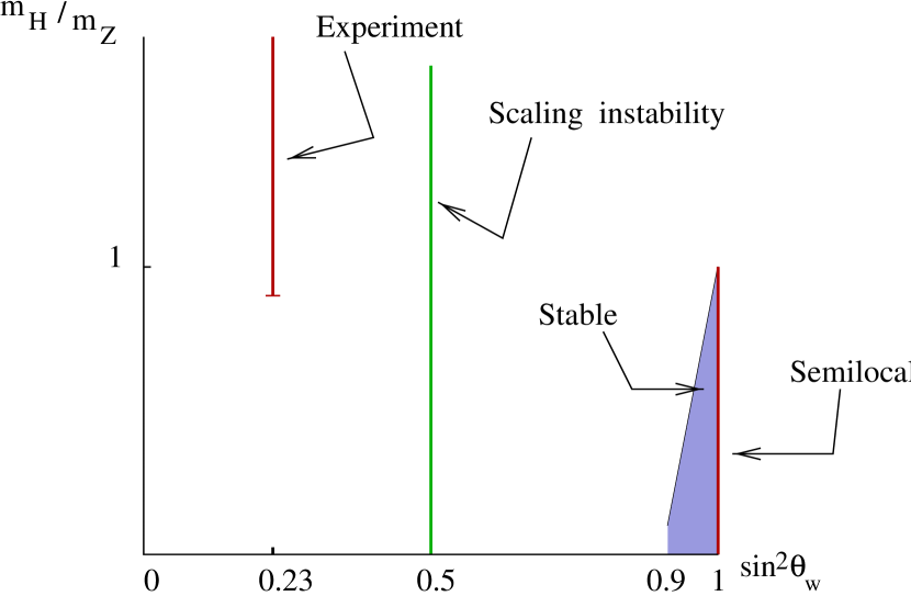
Figure 11: The Z-string is stable in the triangular shaded region of parameter space. At $\sin^{2}\theta_{w}=0.5$, the string has a scaling instability. The experimentally allowed parameters are also shown.

The stability analysis of the Z-string described above leaves open the possibility that the string might be stable in some special circumstances such as, the presence of extra scalar fields, or a magnetic field background, or fermions. We now describe some circumstances in which the Z-string stability has been analyzed.

7.3 Z-string stability continued

The stability of Z-strings has been studied in various other circumstances:

(i) Thermal effects: In [61] the authors examined thermal effects on Z-string stability using the high temperature effective potential and found slight modifications to the stability. The conclusion is that Z-strings in the GSW model are unstable at high temperatures as well. In the same paper, left-right symmetric models were studied and it was found that these could contain stable strings that are similar to the Z-string.

(ii) Extra scalar fields: It is natural to wonder if the presence of extra scalar fields in the model can help provide stability. In [37] the stability was examined in the physically motivated two Higgs doublet model with little advantage. In [126] it was shown that an extra (globally) charged scalar field could enhance stability. The extra complex scalar field, $\psi$, is coupled to the electroweak Higgs by a term $|\psi|^{2}\Phi^{\dagger}\Phi$ and hence the charges have lower energy on the string where $\Phi^{\dagger}\Phi\sim 0$ than outside the string where $\Phi$ has a non-zero VEV. the background of a string and hence a sufficient amount of charge can stabilize the string. This is exactly as in the case of non-topological solitons or Q-balls [108, 44, 31]. However, scalar global charges attract and this can cause an instability of the charge distribution along the string [32, 126]. For realistic parameters, stable Z-strings do not seem likely even in the presence of extra scalar fields.

(iii) Adjoint scalar field: A possible variant of the above scheme is that an $SU(2)$ adjoint can be included in the GSW model as described in Sec. (6.2). Now, since the Z-string is topological within the second symmetry breaking stage in eq. (128), it is stable. However, to be consistent with current experimental data the VEV of the $SU(2)$ adjoint must vanish at a lower energy scale. At this stage the Z-string becomes unstable. Hence, in this scheme, there could be an epoch in the early universe where Z-strings would be stable.

(iii) External magnetic field: An interesting possibility was studied by Garriga and Montes [47] when they considered the stability of the Z-string placed in an external electromagnetic magnetic field of field strength $B$ parallel to the string. First, note that $B$ should be less than $B_{c}=m_{W}^{2}/e$, otherwise the vacuum outside the string is unstable to W-condensation [12]. Then they found that the Z-string could be stable if $B>\sqrt{\beta}B_{c}$, where $\beta=m_{H}^{2}/m_{Z}^{2}$ should be less than 1 for stability of the ambient vacuum. The region of stability for a few values of the magnetic field (given by $K=g_{z}B/2m_{Z}^{2}$) is sketched in Fig. 12. For a certain range of $K\sim 0.85$, stable Z-strings in the GSW model are still just possible.

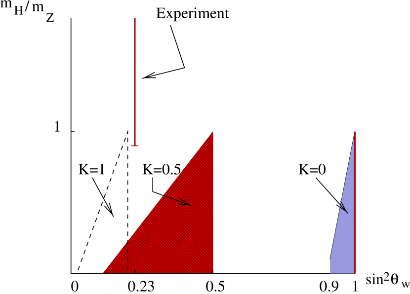
Figure 12: The triangular regions depict the parameter range for which the electroweak vacuum and the Z-string are both stable in the presence of a uniform external magnetic field whose strength is proportional to $K$. For a range of magnetic field ($K\sim 0.85$), stable strings are possible even with the experimentally constrained parameter values.

A way to understand the enhanced stability of the Z-string in a magnetic field is to realize that the W-condensation instability is due to the interaction of $W^{3}_{\mu}=\sin\theta_{w}A_{\mu}+\cos\theta_{w}Z_{\mu}$ and $W^{\pm}_{\mu}$. The Z-string itself has a Z magnetic flux. Then the external electromagnetic flux can serve to lower the net $W^{3}$ flux. This reduces the efficiency of W-condensation and makes the string more stable. Another viewpoint can be arrived at if we picture the Z-string instability to be one in which the string breaks due to the production of a monopole- antimonopole pair on the string. If the external magnetic field is oriented in a direction that prevents the nucleated magnetic monopoles from accelerating away from each other, it will suppress the monopole pair production process, leading to a stabilization of the string for sufficiently strong magnetic fields.

(iv) Fermions: The effect of fermions on the stability of the Z-string has been considered in Refs. [38, 93, 77, 84]. Naculich [93] found that fermions actually make the Z-string unstable. In [84] it was argued that this effect of fermions is quite general and also applies to situations where the strings form at a low energy scale due to topological reasons but can terminate on very massive monopoles formed at a very high energy scale. This most likely indicates that the Z-string solution itself should be different from the Nielsen-Olesen solution when fermions are included. We shall describe these results in greater detail in Sec. 8 after discussing fermion zero modes on strings.

Z-strings have also been considered in the presence of a cold bath of fermions [23]. The effect of the fermions is to induce an effective Chern-Simons term in the action which then leads to a long range magnetic field around the string.

7.4 Semiclassical stability

Preskill and Vilenkin [104] have calculated the decay rate of electroweak strings in the region of parameter space where they are classically stable. The instability is due to quantum tunneling and is calculated by finding the semiclassical rate of nucleation of monopole-antimonopole pairs on electroweak strings. The bounce action is found to be

$$S\sim{{4\pi^{2}}\over{g^{2}}}{{a_{\infty}}\over{a_{s}}}$$ (167)

where, the strings are classically stable if the ratio of parameters ${{a_{\infty}}/{a_{s}}}$ is larger than 1. ($a_{\infty}/a_{s}$ is the ratio of energy in the magnetic flux when it is spread over an infinite area to that if it is confined within the string.) The semiclassical decay probability of the string per unit length per unit time is proportional to $\exp[-S]$.

The decay rate gets suppressed as we approach the semilocal string ($g\rightarrow 0$) thus the semilocal string is also stable semiclassically.

8 Superconductivity of electroweak strings

8.1 Fermion zero modes on the Z-string

Here we shall consider the fermionic sector of the GSW model in the fixed background of the unit winding Z-string for which the solution is given in eq. (82). The Dirac equations for a single family of leptons and quarks are obtained from the Lagrangian in Sec. 1.1.2. These have been solved in the background of a straight Z string in [38, 48, 92]. The analysis is similar to that for $U(1)$ strings [64] since the Z-string is an embedded $U(1)$ string in the GSW model (see Sec. 5.3). A discussion of the fermion zero modes in connection with index theorems can be found in [76, 73]

In polar coordinates with the Z-string along the $z$-axis, a convenient representation for the $\gamma$ matrices is:

$$\gamma^{\rho}=\pmatrix{0&e^{-i\varphi}&0&0\cr-e^{i\varphi}&0&0&0\cr 0&0&0&-e^{-i\varphi}\cr 0&0&e^{i\varphi}&0\cr}\ ,\ \ \ \gamma^{\varphi}=\pmatrix{0&-ie^{-i\varphi}&0&0\cr-ie^{i\varphi}&0&0&0\cr 0&0&0&ie^{-i\varphi}\cr 0&0&ie^{i\varphi}&0\cr}\ ,$$ (168)

$$\gamma^{t}=\pmatrix{\tau^{3}&0\cr 0&-\tau^{3}\cr}\ ,\ \ \ \gamma^{z}=\pmatrix{0&{\bf 1}\cr-{\bf 1}&0\cr}\ ,\ \ \ \gamma^{5}=\pmatrix{0&{\bf 1}\cr{\bf 1}&0\cr}\ .$$ (169)

(Note that the derivative $\gamma^{\mu}\partial_{\mu}$ is given by $\gamma^{t}\partial_{t}+\gamma^{\rho}\partial_{\rho}+\gamma^{\phi}\partial_{\phi}/\rho+\gamma^{z}\partial_{z}$.) Then the electron has a zero mode solution

$$e_{L}=\pmatrix{1\cr 0\cr-1\cr 0\cr}\psi_{1}(\rho)\ ,\ \ \ e_{R}=\pmatrix{0\cr 1\cr 0\cr 1\cr}i\psi_{4}(\rho)$$ (170)

where,

$$\psi_{1}^{\prime}+{{qv}\over\rho}\psi_{1}=-h{\eta\over\sqrt{2}}f\psi_{4}$$ (171)

$$\psi_{4}^{\prime}-{{(q-1)v}\over\rho}\psi_{4}=-h{\eta\over\sqrt{2}}f\psi_{1}\ .$$ (172)

In these equations $q$ is the eigenvalue of the operator ${\bf q}$ defined in eq. (87) and denotes the Z-charge of the various left-handed fermions. (For the electron, $q=\cos(2\theta_{w})$.) The boundary conditions are that $\psi_{1}$ and $\psi_{4}$ should vanish asymptotically. This means that there is only one arbitrary constant of integration in the solution to eqns. (171) and (172). This may be taken to be a normalization of $\psi_{1}$ and $\psi_{4}$.

For the $d$ quark, the solution is the same as in eqns. (170), (171) and (172) except that $q=1-(2/3)\sin^{2}\theta_{w}$. For the $u$ quark the solution is:

$$u_{L}=\pmatrix{0\cr 1\cr 0\cr-1\cr}\psi_{2}(\rho)\ ,\ \ \ u_{R}=\pmatrix{1\cr 0\cr 1\cr 0\cr}i\psi_{3}(\rho)$$ (173)

where,

$$\psi_{2}^{\prime}-{{qv}\over\rho}\psi_{2}=-G_{u}{\eta\over\sqrt{2}}f\psi_{3}$$ (174)

$$\psi_{3}^{\prime}+{{(q+1)v}\over\rho}\psi_{3}=-G_{u}{\eta\over\sqrt{2}}f\psi_{2}$$ (175)

where, $q=-1+(4/3)\sin^{2}\theta_{w}$. Note that (171), (172) are related to (174), (175) by $q\rightarrow-q$.

The right-hand sides of the neutrino Dirac equations (corresponding to eqns. (171) and (172)) vanish since the neutrino is massless. The solutions can be found explicitly in terms of the string profile equations in the case when the Higgs boson mass ($m_{H}=\sqrt{2\lambda}\eta$) equals the Z boson mass ($m_{Z}=g_{z}\eta/2$) [48]. Recall that the string equations in the $m_{H}=m_{Z}$ case are [25]:

$$f^{\prime}={f\over\rho}(1-v)$$ (176)

$$v^{\prime}={{m_{Z}^{2}}\over 2}\rho(1-f^{2})$$ (177)

yielding the useful relation:

$$\int d\rho{v\over\rho}={\rm ln}\biggl{(}{m_{Z}\rho\over f}\biggr{)}$$ (178)

where we have included a factor of $m_{Z}$ to make the argument of the logarithm dimensionless. Now the zero mode profile functions for the massless fermions are:

$$\psi_{1}=c_{1}m_{Z}^{3/2}\biggl{(}{{m_{Z}\rho}\over f}\biggr{)}^{-q}\ ,\ \ \ \psi_{4}=c_{4}m_{Z}^{3/2}\biggl{(}{{m_{Z}\rho}\over f}\biggr{)}^{q-1}$$ (179)

where, $c_{1}$ and $c_{4}$ are independent constants that can be chosen to normalize the left- and right-handed fermion states and the spinors are given in (170). The boundary condition that the left-handed fermion wavefunction should vanish at infinity is only satisfied if $q>0$. Hence (179) can only give a valid solution for $q>0$ for the left-handed fermion. If we also require normalizability, we need $q>1$. (Note that there is no singularity at $\rho=0$ because $f\propto\rho$ when $\rho\sim 0$.) If we have a left-handed fermion with $q\leq-1$, the correct equations to use are the equations corresponding to the up quark equations given in (174) and (175) and these are solved by letting $q\rightarrow-q$ in (179). In this case, the spinors are given in (173).

For the electroweak neutrino, the right-handed component is absent and $q=-1$. This means that the neutrino has the same spinor structure as the left-handed up quark and the solution is that in (179) with $q$ replaced by $+1$. Therefore the wave function falls off as $1/\rho$ and the state is strictly not normalizable - the normalization integral diverges logarithmically. However, depending on the physical situation, one could be justified in imposing a cut-off. For example, when considering closed loops of string, the cutoff is given by the radius of the loop.

Next we give the explicit solutions to the Dirac equations in (171) and (172) in the case when the fermion mass ($m_{f}=h\eta/\sqrt{2}$) is equal to the scalar mass which is also equal to the vector mass. This so-called “super-Bogomolnyi” limit is not realized in the GSW model but may be of interest in other situations (for example, in supersymmetric models). Then, if the charge on the left-handed fermion vanishes ($q=0$), the solution can be verified to be:

$$\psi_{1}(\rho)=Nm_{Z}^{3/2}(1-f(\rho)^{2})$$ (180)

$$\psi_{4}(\rho)=2Nm_{Z}^{1/2}{f(\rho)\over\rho}(1-v(\rho))$$ (181)

where $N$ is a dimensionless normalization factor. For the same set of parameters, the solution for the up quark equations can be written by using the transformation $q\rightarrow-q$ in the above solutions. Further, this solution can also be derived using supersymmetry arguments [127, 33].

The left-handed fermion wave-functions found above can be multiplied by a phase factor ${\rm exp}[i(E_{p}t-pz)$ and the resulting wave-function will still solve the Dirac equations provided

$$E_{p}=\epsilon_{i}p$$ (182)

where, $i$ labels the fermions, and,

$$\epsilon_{\nu}=+1=\epsilon_{u}\ ,\ \ \ \epsilon_{e}=-1=\epsilon_{d}\ .$$ (183)

In other words, $\nu_{L}$ and $u$ travel parallel to the string flux while $e$ and $d$ travel anti-parallel to the string flux.

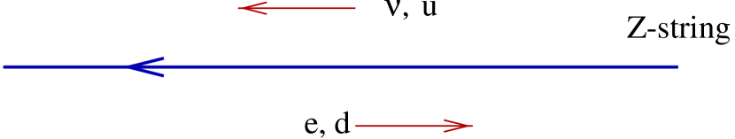
Figure 13: The direction of propagation of quark and lepton zero modes on the Z-string.

We should mention that the picture of quarks travelling along the Z-string may be inaccurate since QCD effects have been totally ignored. At the present time it is not known if the strong forces of QCD will confine the quarks on the string into mesons and baryons (for example, pions and protons). Further, the electromagnetic interactions of the particles on the string might lead to bound states of electrons and protons on the string. This would imply a picture where hydrogen (and other) atoms are the fundamental entities that live on the string.

8.2 Stability of Z-string with fermion zero modes

In Fig. 14 we show the effect that perturbations of order $\epsilon$ in the Z-string fields have on the fermion (u and d quarks) zero modes. The zero momentum modes acquire an $O(\epsilon)$ mass while the non-zero momentum modes get an $O(\epsilon^{2})$ mass. For the perturbation analysis to make sense, we require that the u and d quark zero momentum modes are either both filled or both empty. In that case, the $O(\epsilon)$ terms in the variation in the energy will cancel and we will be left with something that is $O(\epsilon^{2})$. In fact,

$$\Delta E=-{{\epsilon^{2}}\over 2}|m_{1}|^{2}L\sum_{k=1}^{N}{1\over k}$$ (184)

where $m_{1}$ is a matrix element having to do with the interactions of the u and d quarks, $L\rightarrow\infty$ is the length of the string on which periodic boundary conditions have been imposed, and $N\rightarrow\infty$ is a cut-off on the energy levels which are labeled by $k$. The crucial piece of this formula is the minus sign which shows that the energy of the string is lowered due to perturbations [93].

In Ref. [84] it was argued that an identical calculation could be done for any classically stable string that could terminate on (supermassive) magnetic monopoles. However, in the low energy theory, the strings are effectively topological and hence, it seems unlikely that fermions can lead to an instability. This suggests that the bosonic string configuration gets modified by the fermions and the stability analysis around the Nielsen-Olesen solution may be inappropriate.

So far, the stability analysis with fermions presented here only considered the zero modes and ignored the infinitely many massive fermion modes. Very recently, Groves and Perkins [55] have analysed the full spectrum of massless and massive fermionic modes in the background of the electroweak string. They then calculate the effect of the Dirac sea on the stability of electroweak strings by calculating the renormalised energy shift of the Dirac sea when a Z-string is perturbed by introducing a non-zero upper component to the Higgs doublet. This energy shift is negative and so destabilises the string, but it is small, leading them to conclude that if positive energy fermionic states are populated, it is conceivable that the total fermionic contribution could be to stabilise the string. This work is still in progress. In the meantime, the stability of Z–strings remains an open question.

Figure 14: The effect of perturbations of the Z-string on fermion zero modes.

8.3 Scattering of fermions off electroweak strings

The elastic scattering of fermions off semilocal and electroweak strings has been considered in [46, 35, 85].

The main feature of the cross section is that the scattering violates helicity [46]. It is straightforward to show that the helicity operator $\Sigma\cdot\Pi$, where $\Sigma^{i}=\epsilon^{ijk}\gamma^{i}\gamma^{j}$ is the spin operator and $\Pi^{i}$ are the canonical momenta, does not commute with the hamiltonian. If $\Phi^{T}=(\phi^{+},\phi^{0})$, the commutator is proportional to $(D\phi^{0})$ terms. Consider for a moment the usual representation of Dirac matrices,

$$\gamma^{0}=\pmatrix{0\ \ \ \ 1\cr 1\ \ \ \ 0}\qquad\qquad\gamma^{i}=\pmatrix{0\ \ -\tau^{i}\cr\tau^{i}\ \ \ \ 0}\qquad\qquad\gamma_{5}=\pmatrix{1\ \ \ \ \ 0\cr 0\ \ -1}$$ (185)

Then, for an incoming electron, one finds

$$[{\rm H},{\Sigma}\cdot{\Pi}]=ih\left(\begin{array}[]{cc}0&\tau^{j}(D^{j}\phi^{0})^{\dagger}\\ \tau^{j}D^{j}\phi^{0}&0\\ \end{array}\right),$$ (186)

where $h$ is the Yukawa coupling and $(D_{j}\phi^{0})$ is given in eq. (86). Therefore helicity-violating processes can take place in the core of the string.

A preliminary calculation by Ganoulis in ref. [46] showed that, for an incoming plane wave, the dominant mode of scattering gives identical cross sections for positive and negative helicity scattered states. More precisely, for an incoming electron plane wave of momentum $k$, energy $\omega$ and positive helicity it was found that, to leading order,

$${d\sigma\over dk}\biggr{|}_{\pm}\sim{1\over k}\left(\omega-k\over 2\omega\right)^{2}\sin^{2}(\pi q_{R})$$ (187)

where $\omega^{2}=k^{2}+m_{e}^{2}$, $q_{R}$ is the Z-charge of the right fermion field, given in eq. (87) (recall that right and left fermion fields have different Z-charges, $q_{R}=q_{L}\pm 1$).

A more detailed calculation was done by Davis, Martin and Ganoulis [35], and later extended by Lo [85], using a ‘top hat’ model

$$f(r)=\cases{0&$r<R$\cr{\eta/\sqrt{2}}&$r>R$\cr}\qquad\qquad\qquad v(r)=\cases{0&\ \ $r<R$\cr{2/g_{z}}&\ \ $r>R$\cr}\ \ ,$$ (188)

which is expected to be a reasonable approximation since the scattering cross section in the case of cosmic strings has been shown to be insensitive to the core model [102]. Note that there is a discontinuous jump in the fermion mass and string flux; however the wave functions are matched so that they are continuous at $r=R$. Note that the left and right fields decouple in the core of the string, so helicity violating processes are concentrated at $r=R$.

The authors of [35, 85] confirmed that, in the massive case, there are helicity-conserving and helicity-flip scattering cross sections of equal magnitude. The latter goes to zero in the massless limit (in that case, the left and right fields decouple, and no helicity violation is possible), suggesting that helicity violation may be stronger at low energies. For “fractional string flux” (i.e. for fractional $q$) the cross section is of a modified Aharonov-Bohm form, and independent of string radius. For integer $q$ it is of Everett form [41] (the strong interaction cross section is suppressed by a logarithmic term).

Another interesting feature has to do with the amplification of the fermionic wave function in the core of the string. Lo [85] has remarked that there is a regime in which the scattering cross section for electroweak strings is much less sensitive to the fermion charge (that is, to $\sin^{2}\theta_{w}$) than for cosmic strings. In contrast with, e.g., baryon number violating processes, which show maximal enhancement only for discrete values of the fractional flux, the helicity violating cross section for electroweak strings in the regime $k\sim m,\ kR<<1$ shows a plateau for $0<\sin^{2}\theta_{w}<1/2$ where amplification is maximal and the cross section becomes of order $m_{f}^{-1}$. This can be traced back to the asymmetry between left and right fields; while the wave function amplification is a universal feature, different components of the fermionic wave function acquire different amplification factors in such a way that the total enhancement of the cross section is approximately independent of the fermionic charge, $q$ (or, equivalently, of $\sin^{2}\theta_{w}$).

Elastic scattering is independent of the string radius for both electroweak and semilocal strings (for integral flux there is only a mild dependence on the radius coming from the logarithmic suppresion factor in the Everett cross section). Since the cross section is like that of $U(1)$ strings, we would expect electroweak and semilocal strings to interact with the surrounding plasma in a way that is analogous to topological strings.

9 Electroweak strings and baryon number

As first shown by Adler [9], and, Bell and Jackiw [17], currents that are conserved in a classical field theory may not be conserved on quantization of the theory. In the GSW model, one such current is the baryon number current and the anomalous current conservation equation is:

$$\partial_{\mu}j^{\mu}_{B}={{N_{F}}\over{32\pi^{2}}}[-g^{2}W^{a}_{\mu\nu}{\tilde{W}}^{a\mu\nu}+{g^{\prime}}{}^{2}Y_{\mu\nu}{\tilde{Y}}^{\mu\nu}].$$ (189)

where $j^{\mu}_{B}$ is the expectation value of the baryon number current operator $\sum_{s}b_{s}:{\bar{\psi}}\gamma^{\mu}\psi:$ where the sum is over all the species of fermions labeled by $s$, $\psi$ is the fermion spinor and $b_{s}$ is the baryon number for species $s$ and the operator product is normal ordered. Also, $N_{F}$ denotes the number of families, and tilde the dual of the field strengths.

The anomaly equation can be integrated over all space leading to

$$\Delta Q_{B}={{N_{F}}\over{32\pi^{2}}}\int dtd^{3}x[-g^{2}W^{a}_{\mu\nu}{\tilde{W}}^{a\mu\nu}+{g^{\prime}}{}^{2}Y_{\mu\nu}{\tilde{Y}}^{\mu\nu}]=\Delta Q_{CS}.$$ (190)

with,

$$Q_{CS}={{N_{F}}\over{32\pi^{2}}}\int d^{3}x\epsilon_{ijk}\biggl{[}g^{2}\biggl{(}W^{aij}W^{ak}-{g\over 3}\epsilon_{abc}W^{ai}W^{bj}W^{ck}\biggr{)}-{g^{\prime}}{}^{2}Y^{ij}Y^{k}\biggr{]}\ .$$ (191)

Here, $\Delta(\cdot)$ denotes the difference of the quantities evaluated at two different times, $Q_{B}$ is the baryonic charge and the surface currents and integrals at infinity are assumed to vanish. $Q_{CS}$ is called the Chern-Simons, or topological, charge and can be evaluated if we know the gauge fields. The left-hand side of eq. (190) evaluates the baryon number by counting the fermions directly. We describe the evaluation of both the right- and left-hand side for fermions on certain configurations of Z-strings in the following subsections. Finally, in Sec. 9.4 we briefly comment on possible applications to cosmology.

9.1 Chern-Simons or topological charge

We will be interested in the Chern-Simons charge contained in configurations of Z-strings. Then, we set all the gauge fields but for the Z-field to zero in the expression for the Chern-Simons charge, yielding

$$Q_{CS}=N_{F}{{\alpha^{2}}\over{32\pi^{2}}}\cos(2\theta_{w})\int d^{3}x{\vec{Z}}\cdot{\vec{B}}_{Z}$$ (192)

where, ${\vec{B}}_{Z}$ denotes the magnetic field in the Z gauge field: $B^{i}_{Z}=\epsilon^{ijk}\partial_{j}Z_{k}$.

The terms on the right-hand side have a simple interpretation in terms of a concept called “helicity” in fluid dynamics [19]. Essentially, if a fluid flows with velocity $\vec{v}$ and vorticity $\vec{\omega}=\vec{\nabla}\times\vec{v}$, then the helicity is defined as:

$$h=\int d^{3}x{\vec{v}}\cdot{\vec{\omega}}$$ (193)

Since the helicity measures the velocity flow along the direction of vorticity, it measures the corkscrew motion (or twisting) of the fluid flow. A direct analog is defined for magnetic fields:

$$h_{B}=\int d^{3}x{\vec{A}}\cdot{\vec{B}}$$ (194)

which is of the same form as the terms appearing in (192). Hence the Chern-Simons charge measures the twisting of the magnetic lines of force. The helicity associated with the Z field alone is given by:

$$H_{Z}=\int d^{3}x{\vec{Z}}\cdot{\vec{B}}_{Z}\ .$$ (195)

If we think in terms of flux tubes of $Z$ magnetic field, $H_{Z}$ measures the sum of the link and twist number of these tubes:

$$H_{Z}=L_{Z}+T_{Z}\ .$$ (196)

For a pair of unit winding Z flux tubes that are linked once as shown in Fig. 15 the helicity is:

$$H_{Z}=2F_{Z}^{2}$$ (197)

where, $F_{Z}$ is the magnetic flux in each of the two tubes Note that the helicity is positive for the strings shown in Fig. 15. If we reversed the direction of the flux in one of the loops, the magnitude of $H_{Z}$ would be the same but the sign would change. For the Z-string, we also know that

$$F_{Z}={{4\pi}\over g_{z}}$$ (198)

and so eq. (192) yields [124]:

$$Q_{CS}=N_{F}\cos(2\theta_{w})\ .$$ (199)

Figure 15: A pair of linked loops.

9.2 Baryonic charge in fermions

The baryon number associated with linked loops of Z-string has been evaluated in Ref. [48] by studying the fermionic zero modes on such loops. This corresponds to evaluating the left-hand side of eq. (190) directly in terms of the fermions that carry baryon number. The calculation involves adding the baryonic charges of the infinite Dirac sea of fermions living on the string together with zeta function regularization.

To understand why the linking of loops leads to non-trivial effects, note that the quarks and leptons have a non-trivial Aharanov-Bohm interaction with the Z-string. So the Dirac sea of fermions on a loop in Fig. 15 is affected by the Z-flux in the second loop. This shifts the level of the Dirac sea in the ground state leading to non-trivial baryonic and other charges.

Instead of considering the linked loops as shown in Fig. 15 it is simpler to consider a large circular loop of radius $a\rightarrow\infty$ in the $xy$-plane threaded by $n$ straight infinite strings along the $z$-axis (Fig. 16). Then the fermionic wave-functions take the form:

$$\psi_{L}=e^{-i(E_{p}t-p\sigma)}\psi_{L}^{(0)}(r)\ ,\ \ \ \psi_{R}=e^{-i(E_{p}t-(p-n/a)\sigma)}\psi_{R}^{(0)}(r)\$$ (200)

where the functions with superscript $(0)$ are the zero mode profile functions described in Sec. 8.1 and $\sigma$ is a coordinate along the length of the circular loop. From these wavefunctions, the dispersion relation for a zero mode fermion on the circular loop is

$$\omega_{k}=\epsilon_{i}(k-qZ)\ .$$ (201)

where, $q$ is the Z-charge of the fermion, $\epsilon_{i}$ is defined in eq. (183), $\omega$ is related to the energy $E$ by $\omega\equiv aE$, and $k$ to the momentum $p$ by $k\equiv ap\in{\rm\angle\!\!\!Z}$. $Z$ is the component of the gauge field along the circular loop multiplied by $a$ and is given by,

$$Z\equiv{{2n}\over{g_{z}}}\ .$$ (202)

The crucial property of the dispersion relation is that, if there is an Aharanov-Bohm interaction between the Z-string and the fermion, $\omega_{k}$ cannot be zero for any value of $k$ since $k$ is an integer but $qZ$ is not.

The Z- , A- and baryon number (B) charges of the leptons and quarks are shown in Table 1. Note that we use $2q_{Z}/g_{z}$ to denote the Z-charge and this is identical to the eigenvalue of the operator ${\bf q}$ defined in eq. 87 and also to $q$ used in the previous section.

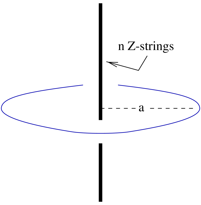
Figure 16: A circular Z-string loop of radius $a$ threaded by $n$ Z-strings.

Table 1: Summary of $Z-$, electric and baryonic charges for the leptons and quarks. The charges $q_{Z}$ are for the left-handed fermions and $s^{2}\equiv\sin^{2}\theta_{w}$.

	$\nu_{L}$	$e$	$d$	$u$
$2q_{Z}/g_{z}$	-1	$1-2s^{2}$	$1-{{2s^{2}}/3}$	$-1+{{4s^{2}}/3}$
$q_{A}/e$	0	-1	$-1/3$	$2/3$
$q_{B}$	0	0	$1/3$	$1/3$

The energy of the fermions is found by summing over the negative frequencies - that is, the Dirac sea - and so the energy $E$ due to a single fermion species is:

$$E={1\over a}\sum\omega_{k}=\epsilon_{i}{1\over a}\sum_{k=k_{F}}^{-\epsilon_{i}\infty}(k-qZ)$$ (203)

where, $k_{F}$ denotes the Fermi level - the value of $k$ for the highest filled state. Therefore we need to sum a series of the type:

$$S=\sum_{k=k_{F}}^{\infty}(k-qZ)=\sum_{k=0}^{\infty}(k+k_{F}-qZ)\ .$$ (204)

The sum is found using zeta function regularization:

$$S=\zeta(-1,k_{F}-qZ)=-{1\over{12}}-{1\over 2}(k_{F}-qZ)(k_{F}-qZ-1)$$ (205)

With this result, the energy contribution from the $i^{th}$ species of fermions takes the form:

$$E_{i}=-{1\over{24a}}+{1\over{2a}}\biggl{[}k_{F}^{(i)}-q_{i}Z+{\epsilon_{i}\over 2}\biggr{]}^{2}\equiv-{1\over{24a}}+{1\over{2a}}K_{i}^{2}\ .$$ (206)

Adding the contributions due to different members of a single fermion family, we get

$$2aE=K_{\nu}^{2}+K_{e}^{2}+3K_{d}^{2}+3K_{u}^{2}\ .$$ (207)

Next we can calculate the angular momentum of the fermions in the circular loop background. The system has rotational symmetry about the $z-$axis and this enables us to define the generalized angular momentum operator as the operator that annihilates the background field configuration [67]:

$$M_{z}=L_{z}+S_{z}+nI_{z}$$ (208)

where,

$$L_{z}=-i{\bf 1}{{\partial\ }\over{\partial\varphi}}\ ,$$ (209)

$S_{z}$ is the spin operator, and, the isospin operator is given in terms of the $U(1)$ (hypercharge) and $SU(2)$ charges - $q_{1}$ and $q_{2}$ respectively - of the field in question:

$$I_{z}={1\over 2}\biggl{[}\biggl{(}{{2q_{2}}\over g}\biggr{)}T^{3}-\biggl{(}{{2q_{1}}\over{g^{\prime}}}\biggr{)}{\bf 1}\biggr{]}\ .$$ (210)

The isopin operator acts via a commutator bracket on the gauge fields and by ordinary matrix multiplication on the Higgs field and fermion doublets.

We are interested in the angular momentum of the chiral fermions on the circular loop which lies entirely in the $xy$-plane. The fermions in the zero modes therefore have $S_{z}=0$. (The spin of the fermions is oriented along their momenta which lies in the $xy$-plane.) The action of $L_{z}$ is found by acting on the fermion wave-functions such as in eq. (200) (remembering to let $n\rightarrow-n$ for the neutrino and up quark). The action of $I_{z}$ is found by using the charges of the fermions given in the GSW model defined in Sec. 1.1.2. We then find:

$$M_{z}\pmatrix{\nu_{L}\cr e_{L}\cr}=\pmatrix{(k^{(\nu)}+n)\nu_{L}\cr k^{(e)}e_{L}\cr}\ ,\ \ \ M_{z}\pmatrix{u_{L}\cr d_{L}\cr}=\pmatrix{(k^{(u)}+{n/3})u_{L}\cr(k^{(d)}-{{2n}/3})d_{L}\cr}\ ,$$ (211)

$$M_{z}e_{R}=k^{(e)}e_{R}\ ,\ \ M_{z}u_{R}=(k^{(u)}+{n/3})u_{R}\ ,\ \ M_{z}d_{R}=(k^{(d)}-{{2n}/3})d_{R}\$$ (212)

where the $k^{(i)}$ are defined above eqn. (201). Now summing over states, as in the case of the energy, we find the total generalized angular momentum of the fermions on the circular loop:

$${\cal M}={1\over 2}\biggl{[}k_{F}^{(\nu)}+n+{1\over 2}\biggr{]}^{2}-{1\over 2}\biggl{[}k_{F}^{(e)}-{1\over 2}\biggr{]}^{2}-{3\over 2}\biggl{[}k_{F}^{(d)}-{{2n}\over 3}-{1\over 2}\biggr{]}^{2}+{3\over 2}\biggl{[}k_{F}^{(u)}+{{n}\over 3}+{1\over 2}\biggr{]}^{2}\ .$$ (213)

Note that though the gauge fields do not enter explicitly in the generalized angular momentum, they do play a role in determining the angular momentum of the ground state through the values of the Fermi levels.

The calculation of the electromagnetic and baryonic charges and currents on the linked loops is similar but has a subtlety. To find the total charge, a sum over the charges in all filled states must be done. This leads to a series of the kind:

$$S_{q}=\sum_{k=k_{F}}^{\infty}1\ .$$ (214)

To regularize the divergence of the series, it is written as

$$S_{q}=\lim_{\lambda\to 0}\sum_{k=k_{F}}^{\infty}(k-qZ)^{\lambda}\ .$$ (215)

The subtlety is that the gauge invariant combination $k-qZ$ is used as a summand rather than $k$ or some other gauge non-invariant expression [91]. Once again zeta function regularization is used to get:

$$S_{q}=\sum_{k=0}^{\infty}(k+k_{F}-qZ)^{0}=\zeta(0,k_{F}-qZ)=-\biggl{[}k_{F}-qZ-{1\over 2}\biggr{]}\ .$$ (216)

With this result, the contribution to the charge due to fermion $i$ is:

$$Q_{i}=\epsilon_{i}{\bar{q}}_{i}\biggl{[}k_{F}^{(i)}-q_{i}Z+{\epsilon_{i}\over 2}\biggr{]}=\epsilon_{i}{\bar{q}}_{i}K_{i}$$ (217)

where, ${\bar{q}}_{i}$ is the charge carried by the $i^{th}$ fermion of the kind that we wish to calculate. (Note that ${\bar{q}}_{i}$ can represent any charge - electric, baryonic etc. - and is, in general, different from the Z-charge $q_{i}$.)

The currents along the string are given by ${\bar{\psi}}\gamma^{z}\psi$ where $\gamma^{z}$ is given in eq. (169). This gives

$$J_{i}=\epsilon_{i}{{Q_{i}}\over{2\pi a}}\ .$$ (218)

By adding the contributions due to each variety of fermion, expressions for the energy, angular momentum, charges and currents for one loop threaded by $n$ have been found in [48]. These results are reproduced in Table 2. It is reassuring to note that in the ground state, the baryon number of the single loop is given by $nN_{F}\cos 2\theta_{W}$ in agreement with the calculation of the Chern-Simons number.

Table 2: Expressions for the energy, generalized angular momentum, charges and currents in terms of $x=2n\sin^{2}\theta_{w}/3$. We have omitted the multiplicative factor $N_{F}$ in all the expressions for convenience.

	$x\in(0,1/3)$	$(1/3,1/2)$	$(1/2,2/3)$	$(2/3,1)$
$aE$	$12x^{2}-6x+1$	$12x^{2}-9x+2$	$12x^{2}-15x+5$	$12x^{2}-18x+7$
$M$	0	$n-1$	$2-n$	0
$Q_{A}/e$	0	-1	+1	0
$B$	$-3x+1$	$-3x+1$	$-3x+2$	$-3x+2$
$2\pi aJ_{A}/e$	$-8x+2$	$-8x+3$	$-8x+5$	$-8x+6$
$2\pi aJ_{B}$	$-x$	$-x$	$1-x$	$1-x$

Figure 17: The energy of the ground state of linked loops versus $x=2n\sin^{2}\theta_{w}/3$.

The energy of the fermionic ground state shows a complicated dependence on $x$ as is demonstrated in Fig. 17. Note that $E(x)$ does not have a monotonic dependence on $x$ and the energy of strings that are linked $n$ times bears no simple relation to those linked $m$ times. In particular, the energy does not continue to decrease as we consider strings that have higher linkage. The lowest energy possible, however, is when $x=1/4$ and for $n=1$, this corresponds to $\sin^{2}\theta_{w}=3/8$, which is also the value set by Grand Unified models. It is not clear if this is simply a coincidence or if there is some deeper underlying reason [70].

9.3 Dumbells

In his 1977 paper, Nambu discussed the possible occurrence of electroweak monopoles and strings in particle accelerators. There are two issues in this discussion: the first is the production crossection of solitonic states in particle collisions, and the second is the signatures of such states if they are indeed produced in an accelerator. The answer to the first question is not known though it is widely believed that the process is suppressed not only by the large amount of energy required but also due to the coherence of the solitonic state. The second question was addressed by Nambu [94] and he estimated the energy and lifetime of electroweak strings that may be possible to detect in accelerators.

To find the energy of a Z-string segment, Nambu treated the monopoles at the ends as hollow spheres of radius $R$ inside which all fields vanish. A straightforward variational calculation in units of $\eta\approx 246$ GeV then gives the monopole mass

$$M={4\pi\over 3e}\sin^{5/2}\theta_{w}\sqrt{m_{H}\over m_{W}}$$ (219)

and radius

$$R=\sqrt{\sin\theta_{w}\over m_{H}m_{W}}$$ (220)

The string segment is approximated by a cylindrical tube with uniform $Z$ magnetic flux with all other fields vanishing. This gives

$$\rho={2\over\sqrt{m_{H}m_{Z}}}\ \ ,\qquad\qquad\tau=\pi\left({m_{H}\over m_{Z}}\right)$$ (221)

for the core radius and string tension, respectively.

Now, if the monopoles are a distance $l$ apart, the total energy of the system is

$$E=2M-{Q^{2}\over 4\pi l}+\tau l$$ (222)

which is clearly minimised by $l=0$ i.e. the string can minimize its energy by collapsing. The tendency to collapse can be countered by a centrifugal barrier if the string segment (“dumbell”) is rotating fast enough about a perpendicular axis. The energy and angular momentum of a relativistic dumbell has been estimated by Nambu to be:

$$E\sim{\mathchoice{{\textstyle{1\over 2}}}{1\over 2}{1\over 2}{1\over 2}}\pi l\tau\qquad L\sim{1\over 8}\pi l^{2}\tau$$ (223)

where,

$${l\tau\over 2M}={v^{2}\over 1-v^{2}}$$ (224)

with $v\sim 1$ being the velocity of the poles. The expressions for $E$ and $L$ imply the existence of asymptotic Regge trajectories,

$$L\sim\alpha_{0}^{\prime}E^{2}$$ (225)

with slope

$$\alpha_{0}^{\prime}={1\over{2\pi\tau}}\sim\left({m_{Z}\over m_{H}}\right){\rm TeV}^{-2}\ .$$ (226)

which, if found, would be a signature of dumbells.

The orbiting poles at the ends of the rotating dumbell will radiate electromagnetically and this energy loss provides an upper bound to the lifetime of the configuration. An estimate of the radiated power from the analysis of synchrotron radiation in classical electrodynamics (eg. see [63]) gives

$$P\sim{{8\pi}\over 3}\times 137\left({\tau\over M}\right)^{2}\sin^{4}\theta_{w}$$ (227)

Therefore the decay width $\Gamma=P/E$ is given by

$$\Gamma\simeq{E\over L}$$ (228)

and for large angular momentum, can lead to significant lifetimes (compared to $E^{-1}$).

To obtain numerical estimates, note that the above estimates are valid only if the dumbell length is much greater than the width of the Z-string. This imposes a lower bound on the angular momentum:

$$L>>{\pi\over 2}\times 137\sin^{2}\theta_{w}\cos^{2}\theta_{w}\sim 36$$ (229)

Using the relation between the energy and the angular momentum, such an object has $E>>6(m_{H}/m_{Z})^{1/2}$ TeV.

The estimates above assume that the lifetime of the dumbell is dictated by the energy emission in photons. In reality, there are other decay channels as well, though it is likely that these will be comparitively suppressed since the photon is the only massless boson present in the system. The dumbell can also decay by fragmenting due to field-theoretic instabilities of the kind discussed in Sec. 7. These may be suppressed due to the finite size of the dumbell, and as Nambu points out, due to the angular momentum of the dumbell . A careful analysis of these factors has not yet been performed and is a vital open problem that may become experimentally relevant with the next generation of accelerators.

9.4 Possible cosmological applications

The role of electroweak strings in cosmology depends on their abundance during and after the electroweak phase transition. If this abundance is negligible, electroweak strings may at best only be relevant in future accelerator experiments (see Sec. 9.3). If, however, there is a cosmological epoch during which segments and loops of electroweak strings were present, they could impact on two observational consequences: the first is the presence of a primordial magnetic field, and the second is the generation of a cosmological baryon number. What is perhaps most remarkable is that the two consequences might be related - the baryonic density of the universe would be related to the helicity of the primordial magnetic field [120, 107].

(i) Primordial magnetic fields: A gas of electroweak segments is necessarily accompanied by a gas of electroweak monopoles. The eventual collapse and disappearance of electroweak strings removes all the electroweak monopoles but the long range magnetic field emanating from the monopoles is expected to remain trapped in the cosmological plasma since that is a very good electrical conductor. This will then lead to a residual primordial magnetic field in the present universe.

A quantitative estimate of the resulting primordial magnetic field cannot be made with confidence but a dimensional estimate is possible. An estimate for the average flux through an area $L^{2}=N^{2}/T^{2}$, where $N$ is a dimensionless number that relates the length scale of interest, $L$, to the cosmological thermal correlation length $T^{-1}$, was obtained in [117, 120], and then translated into the average magnetic field through that area. The result is:

$$B|_{area}\sim T^{2}/N\ .$$ (230)

(Magneto-hydrodynamical considerations provide a lower bound $\sim 10^{12}$ cms on $L$ at the present epoch.) It is important to remember that the above is an areal (i.e. flux) average, defined by [40]

$$B|_{area}\equiv\biggl{\langle}\biggl{(}{1\over A}\int d{\vec{S}}\cdot{\vec{B}}\biggr{)}^{2}\biggr{\rangle}^{1/2}$$ (231)

where the surface integral is over an area $A$ and $\langle\cdot\rangle$ denotes ensemble averaging.

(ii) Baryon number: A gas of electroweak string segments and loops would, in general, contain some helicity density of the Z-field. When the electroweak strings eventually annihilate, it is possible that the helicity gets converted into baryon number [124, 120]. However, in Ref. [42, 43] it is argued that fractional quantum numbers of a soliton are unrelated to the number of particles produced when the soliton decays. Instead, only the change in the winding of the Higgs field in a process that starts out in the vacuum and ends up in the vacuum can be related to the particle number. This would imply that we would have to consider the formation of electroweak strings together with their decay before we can find the resulting baryon number. Such a calculation has not yet been attempted.

An interesting question is to consider what happens to the helicity in the Z-field after the strings disappear. One possibility is that the helicity gets transferred to a frozen-in residual magnetic field after the strings have decayed. To see this, consider a linked pair of loops as in Fig. 15. The strings can break by nucleating monopole-antimonopole pairs, and then the string segments can shrink, finally leading to monopole annihilation. If this process happens in the early universe, the loops will be surrounded by the ambient plasma which will freeze-in the magnetic field lines. Hence, after the strings have disappeared, we will be left with a linked pair of magnetic field lines. In other words, the original helicity in the Z-field has been transferred to helicity in the A-field. This argument relies on the freezing-in of the magnetic field emanating from the monopoles and in the real setting the physics can be much more complicated. However, a connection between the baryon abundance of the universe and the properties of a primordial magnetic field seems tantalizing.

Stable strings at the electroweak scale: If in more exotic models, strings at the electroweak scale were stable and had the superconducting properties discussed above, they could be responsible for baryogenesis [14] and the presence of primary antiprotons in cosmic rays [113]. The production of antiprotons follows on realizing that any strings tangled in the galactic plasma would be moving across the galactic magnetic field. In the rest frame of the string, the changing magnetic field causes an electric field along the string according to Faraday’s law. The electric field along the string raises the levels of the u- and d-quark Dirac seas (see Fig. 18), as well as the electron Dirac sea (not shown in the figure). This means that the electric field produces quarks and leptons on the string. The electric charges of the particles are in the ratio $e:u:d::-1:+2/3:-1/3$ and the rate of production of these particles due to the applied electric field is proportional to the charges. Furthermore, the quarks come in three colors and so for every electron that is produced, $3\times 2/3=2$ u-quarks and $3\times 1/3=1$ d-quark are also produced. As a result, the net electric charge produced is $1\times(-1)+2\times(2/3)+1\times(-1/3)=0$. However, net baryon number $2\times(1/3)+1\times(1/3)=1$ is produced because the quarks carry baryonic charge $1/3$ while the baryonic charges of the leptons vanish. Depending on the orientation of the string, either baryons or antibaryons will be produced. Some of these would then be emitted from the string and would arrive on earth as cosmic rays.

Formation of strings in the electroweak phase transition. Early attempts to understand the formation rates of electroweak strings were made in [120] based on the statistical mechanics of strings. The estimates indicate that a density of strings will be formed immediately after the phase transition. However, the application of string statistical mechanics to electroweak strings may not be justified and so other avenues of investigation are needed. An alternative approach to study electroweak string formation was taken by Nagasawa and Yokoyama [98]. They assumed a thermal distribution of scalar field values and gradients, and estimated the probability of obtaining a string-like scalar field configuration. The conclusion was that electroweak vortex formation in a thermal system is totally negligible. One possible caveat is that the technique used in [98] ignores the effect of gauge fields, which we know are significant in the formation of related objects such as semilocal strings. In [110], Saffin and Copeland have evolved the classical equations of motion to study the formation of electroweak strings, and they found the presence of the gauge fields led to larger string densities than one would have inferred from the scalar fields alone, at least when $\sin^{2}\theta_{w}=0$. However, this study does not directly address the question of string formation in a phase transition because no measure has been placed on the choice of initial conditions and their choice may be too restrictive. Most recently, a promising development has taken place [27] - calculations in lattice gauge theory have been done to study the electroweak phase transition and there is evidence that electroweak strings will form. Further studies along these lines will provide important and quantitative insight into the formation of electroweak strings.

Using the results on the formation of semilocal strings, we can gain some intuition about the formation of electroweak strings in the region of parameter space close to the semilocal limit (the region of stability in Fig. 11). We have seen that semilocal strings with $\beta<1$ have a non-zero formation rate, increasing as $\beta\to 0$. Initially short segments of string are seen to grow and join nearby ones because this reduces the gradient energy at the ends of the strings. The ends of electroweak strings are proper magnetic monopoles, and therefore the scalar gradients are cancelled much more efficiently by the gauge fields, but as $\sin\theta_{w}\to 0$ the cores of the monopoles get larger and larger, and they could begin to overlap with nearby monopoles, so it is possible that short segments of electroweak string will also grow into longer ones.

Figure 18: The dispersion relations for the u and d quark zero modes are shown. The filled states are denoted by solid circles while dashes denote unfilled states. For convenience, periodic boundary conditions are assumed along the string and so the momentum takes on discrete values.

10 Electroweak strings and the sphaleron

The sphaleron is a classical solution in the GSW model that carries baryon number $N_{F}/2$, where $N_{F}$ is the number of fermion families [90, 74]. For $\theta_{w}=0$, the asymptotic form of the sphaleron Higgs field is:

$$\Phi_{sph}=\pmatrix{\cos\theta\cr\sin\theta~{}e^{i\varphi}\cr}\ .$$ (232)

while the gauge fields continue to be given by eq. (100)-(101) in which ${\bar{\Phi}}$ should be replaced by $\Phi_{sph}$. (Note that the hypercharge gauge field vanishes for $\theta_{w}=0$.) Inside the sphaleron, the Higgs field vanishes at one point. The sphaleron also has a magnetic dipole moment that has been evaluated for small values of $\theta_{w}$. The reason that the sphaleron is important for particle physics is that its energy defines the minimum energy required for the classical violation of baryon number in the GSW model.

As has already been described in Sec. 9, non-trivial baryon number can be associated with linked and twisted segments of electroweak string. Further, for specific values of the link and twist, the baryon number of a configuration of Z-strings can also be $N_{F}/2$. This raises the question: are sphalerons related to Z-string segments?

An early paper to draw a connection between the various solutions in the GSW model is Ref. [45]. In [124, 60, 120, 59], however, a direct correspondence between the field configuration of the Z-string and the sphaleron was made.

10.1 Content of the sphaleron

In [60] Hindmarsh and James evaluated the magnetic charge density and current density within the sphaleron. A subtlety in this calculation is that there is no unique definition of the electromagnetic field when the Higgs field is not everywhere in the vacuum. The choice adopted in [60] (and also the choice in this review) is

$$F_{ij}^{em}=\sin\theta_{w}W_{ij}^{a}n^{a}+\cos\theta_{w}Y_{ij}\ .$$ (233)

The evaluation of the magnetic charge density (which is proportional to the divergence of the magnetic field strength) clearly shows that the sphaleron contains a region with positive magnetic charge density and a region with negative magnetic charge density. Furthermore, the total charge in, say, the positive charge region agrees with the magnetic charge of a monopole. In addition, there is a flux of Z magnetic field connecting the two hemispheres. This would seem to confirm that the sphaleron consists of a Z-string segment. However, this is not the full picture. In addition to the string segment, Hindmarsh and James find that the electric current is non-zero in the equatorial region and is in the azimuthal (${\hat{e}}_{\varphi}$) direction.

10.2 From Z-strings to the sphaleron

The scalar field configuration for a finite segment of Z-string was given in Sec. 9.3:

$$\Phi_{m\bar{m}}=\pmatrix{\cos(\Theta/2)\cr\sin(\Theta/2)~{}e^{i\varphi}\cr}$$ (234)

where,

$$\cos\Theta\equiv\cos\theta_{m}-\cos\theta_{\bar{m}}+1$$ (235)

and the angles $\theta_{m}$ and $\theta_{\bar{m}}$ are measured from the monopole and antimonopole respectively, as shown in Fig. 19.

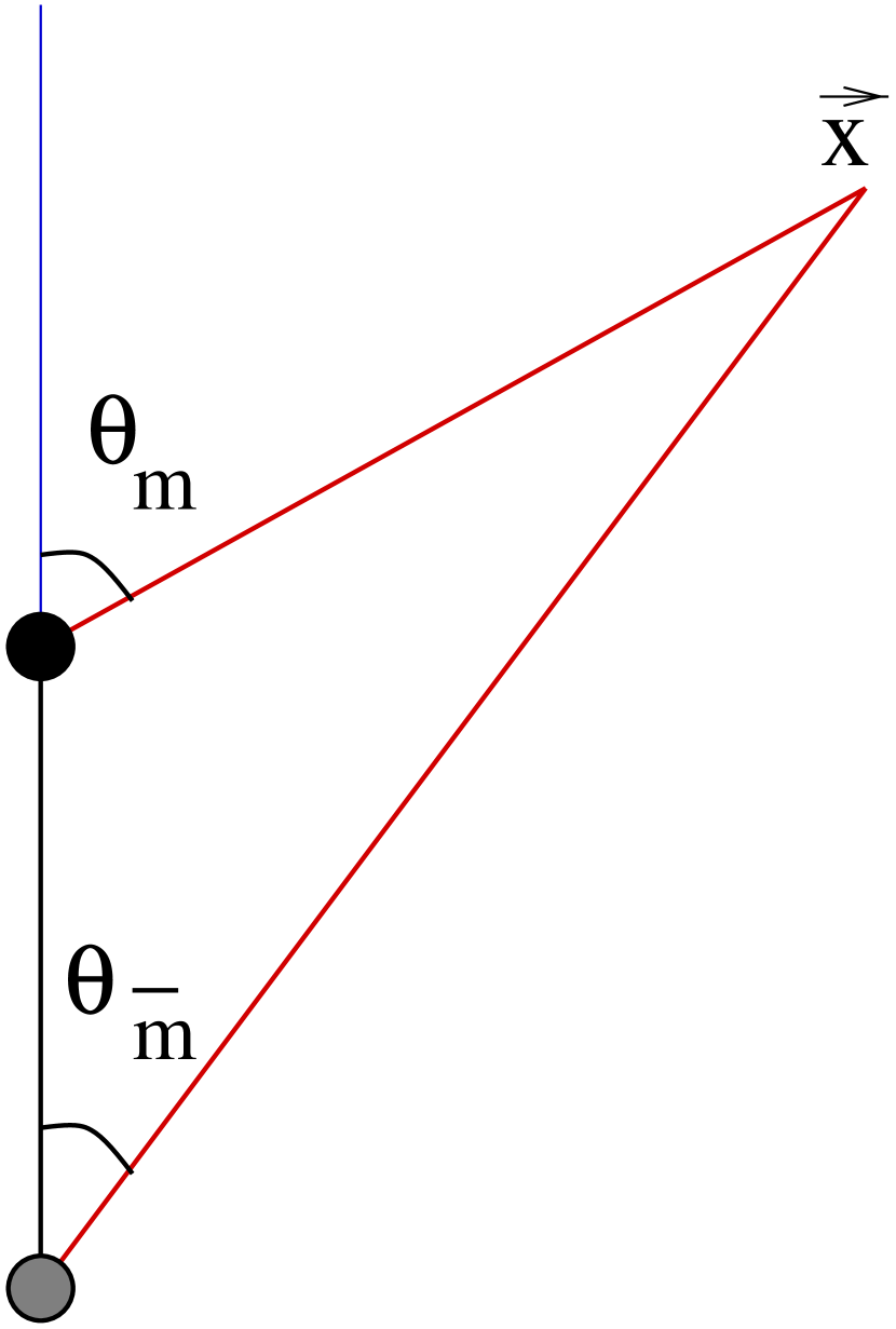
Figure 19: Definition of the coordinate angles $\theta_{m}$ and $\theta_{\bar{m}}$. The azimuthal angle, $\varphi$, is not shown.

It is straightforward to check that (234) yields the monopole field configuration close to the monopole ($\theta_{\bar{m}}\rightarrow 0$) and the antimonopole configuration close to the antimonopole ($\theta_{m}\rightarrow\pi$). It also yields a string singularity along the straight line joining the monopole and antimonopole ($\theta_{m}=\pi,~{}\theta_{\bar{m}}=0$). However, there are other Higgs field configurations that also describe monopoles and antimonopoles:

$$\Phi_{m}=e^{i\gamma}\pmatrix{\cos(\theta_{m}/2)\cr\sin(\theta_{m}/2)~{}e^{i\varphi}\cr}\ ,\ \ \ \ \Phi_{\bar{m}}=e^{i\gamma}\pmatrix{\sin(\theta_{\bar{m}}/2)\cr\cos(\theta_{\bar{m}}/2)~{}e^{i\varphi}}\ .$$ (236)

Next consider the Higgs field configuration:

$$\Phi_{m\bar{m}}(\gamma)=\pmatrix{\sin(\theta_{m}/2)\sin(\theta_{\bar{m}}/2)e^{i\gamma}+\cos(\theta_{m}/2)\cos(\theta_{\bar{m}}/2)\cr\sin(\theta_{m}/2)\cos(\theta_{\bar{m}}/2)e^{i\varphi}-\cos(\theta_{m}/2)\sin(\theta_{\bar{m}}/2)e^{i(\varphi-\gamma)}\cr}$$ (237)

together with the gauge fields given by eq. (100)-(101) with ${\bar{\Phi}}$ replaced by $\Phi_{m\bar{m}}(\gamma)$. When we take the limit $\theta_{\bar{m}}\rightarrow 0$ we find the monopole configuration (with $\gamma=0$) and when we take $\theta_{m}\rightarrow\pi$ the configuration is that of an antimonopole (with arbitrary $\gamma$) provided we perform the spatial rotation $\varphi\rightarrow\varphi+\gamma$. Note that the asymptotic gauge fields agree since these are determined by the Higgs field. The monopole and antimonopole in (237) also have the usual string singularity joining them. This means that the configuration in eq. (237) describes a monopole and antimonopole pair that are joined by a Z-string segment that is twisted by an angle $\gamma$. The Chern-Simons number of one such segment can be calculated [124] and is

$$Q_{CS}=N_{F}\cos 2\theta_{w}~{}{{\gamma}\over{2\pi}}\ .$$ (238)

If $\gamma=\pi/\cos(2\theta_{w})$ then the Chern-Simons number of the twisted segment of string is $N_{F}/2$ and is precisely that of the sphaleron.

Given that the segment with twist $\pi/\cos(2\theta_{w})$ has Chern-Simons number equal to that of the sphaleron, it is natural to ask if some deformation of it will yield the sphaleron. This deformation is not hard to guess for the $\theta_{w}=0$ case. In this case, if we let the segment size shrink to zero, we have $\theta_{m}=\theta_{\bar{m}}=\theta$ and the Higgs field configuration of eq. (237) gives:

$$\Phi_{m\bar{m}}(\gamma=\pi)=\pmatrix{\cos\theta\cr\sin\theta~{}e^{i\varphi}\cr}\ .$$ (239)

This is exactly the scalar field configuration of the sphaleron for $\theta_{w}=0$ (eq. (232)). Note that the asymptotic gauge fields continue to be given by eq. (100)-(101) and satisfy the requirement that the covariant derivatives of the Higgs field vanish.

Encouraged by this successful connection in the $\theta_{w}=0$ case, it was conjectured in [124, 120] that the sphaleron can also be obtained by collapsing a twisted segment of Z-string with Chern-Simons number $N_{F}/2$ for any $\theta_{w}$. If true, this would mean that the asymptotic Higgs field configuration, $\Phi_{S}$, for the sphaleron for arbitrary $\theta_{w}$ is given by

$$\Phi_{S}=\pmatrix{\sin^{2}(\theta/2)~{}e^{i\gamma_{S}}+\cos^{2}(\theta/2)\cr\sin(\theta/2)\cos(\theta/2)~{}e^{i\varphi}(1-e^{-i\gamma_{S}})\cr}$$ (240)

where $\gamma_{S}=\pi/\cos(2\theta_{w})$.

The twisting of the magnetic field lines in the sphaleron configuration has been further clarified in [59]. The direction of magnetic field lines is shown for a dumbell in Fig. 20 and for a “stretched” sphaleron in Fig. 21. (The asymptotic fields for the stretched sphaleron are identical to those for the sphaleron and the twisted Z-string.) In the stretched sphaleron case, the magnetic field line twists around the vertical string segment by an angle $\pi$ (for $\theta_{w}\rightarrow 0$) as one goes from monopole to antimonopole. This twist provides non-trivial Chern-Simons number to the configuration [124].

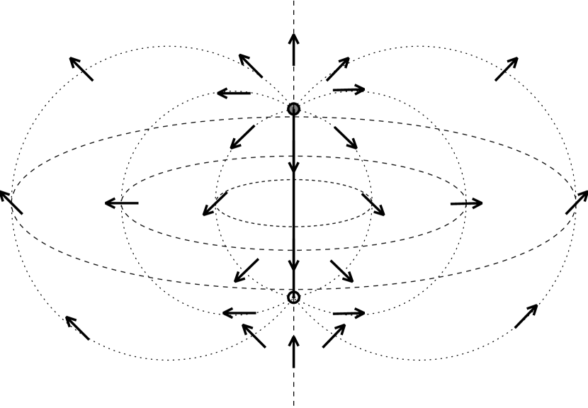
Figure 20: The thick solid line is the location of the Z-string for a dumbell configuration and the dashed curves lie in the equatorial plane and are drawn to guide the eye. The dotted lines depict lines of magnetic flux. The arrows show the orientation of the vector ${\hat{n}}\propto-\Phi^{{\dagger}}{\vec{\tau}}\Phi$.

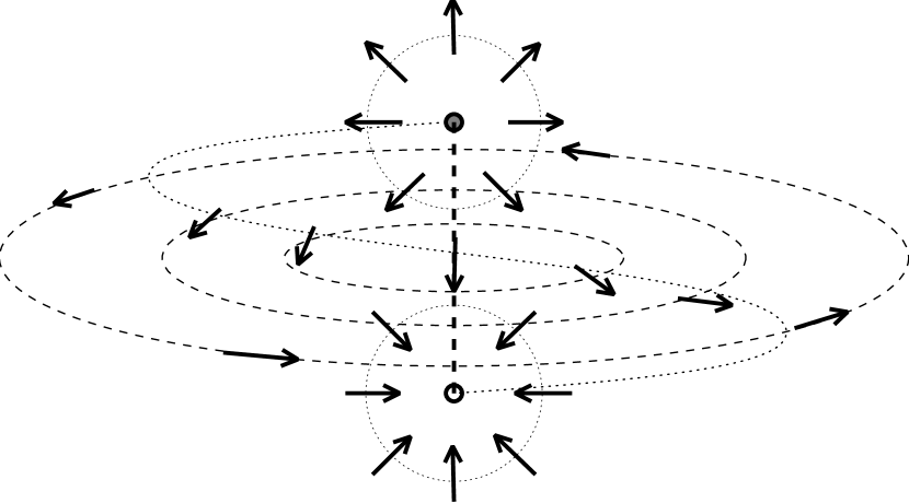
Figure 21: The field configuration for a stretched sphaleron as in Fig. 20. Only one magnetic field line is shown.

On physical grounds it seems reasonable that there should be a critical value of twist at which one can get a static solution for a Z-string segment. This is because the segment likes to shrink under its own tension but the twist prevents the shrinkage and is equivalent to a repulsive force between the monopole and antimonopole. (This idea owes its origin to Taubes [114] who discovered a solution containing a monopole and an antimonopole in an O(3) model in which the Coulomb attraction is balanced by the relative misorientation of the magnetic poles.) Then, if the string is sufficiently twisted, the attractive force due to the tension and the repulsive force due to the twist will balance and a static solution can exist. So far we have been assuming that the only dynamics of the segment is towards collapsing or expanding of the string segment. However, since we are dealing with twisted segments, we should also include the rotational dynamics associated with twisting and untwisting. So, while any twist greater than a certain critical twist might successfully prevent the segment from collapsing, only a special value of the twist can give a static solution to the rotational dynamics. Furthermore, we expect that this solution will be unstable towards rotations that twist and untwist the string segment. This would be the unstable mode of the sphaleron.

Similar connections between the W–string and the sphaleron have also been constructed in [13].

11 The ³He analogy

The symmetry structure of ³He closely resembles the electroweak symmetry group and hence we expect the analog of electroweak strings to exist in ³He [133, 130, 132]. Indeed, this analog is called the $n=2$ vortex. We now explain this correspondence in greater detail.

11.1 Lightning review of ³He

³He nuclei have spin $1/2$ and two such nuclei form a Cooper pair which is the order parameter for the system. Unlike ⁴He, the pairing is a spin triplet ($S=1$) as well as an orbital angular momentum triplet ($L=1$). As a result there are $3\times 3$ components of the wavefunction of the Cooper pair - that is the order parameter has 9 complex components. Hence, the order parameter is written as a 3 by 3 complex valued matrix: $A_{\alpha i}$ with $\alpha$ (spin index) and $i$ (spatial index) ranging from 1 to 3.

At temperatures higher than a few milli Kelvin the system is invariant under spatial rotations ($SO(3)_{L}$) as well as rotations of the spin degree of freedom of the Cooper pair ($SO(3)_{S}$). Another symmetry is under overall phase rotations of the wavefunction ($U(1)_{N}$) and the corresponding conserved charge is particle number ($N$). Hence the symmetry group is:

$$G=SO(3)_{L}\times SO(3)_{S}\times U(1)_{N}\ .$$ (241)

There are several possible phases of ³He corresponding to different expectation values of the order parameter. In the A-phase, the orbital angular momenta of the Cooper pairs are all aligned and so are the spin directions. This corresponds to

$$A_{\alpha i}=\Delta_{0}{\hat{d}}_{\alpha}\psi_{i}$$ (242)

where $\Delta_{0}\sim 10^{-7}$ eV is the temperature dependent gap amplitude, the real unit vector ${\hat{d}}_{\alpha}$ is the spin part of the order parameter, and

$$\psi_{i}={{{\hat{m}}_{i}+i{\hat{n}}_{i}}\over{\sqrt{2}}}$$ (243)

with ${\hat{m}}$ and ${\hat{n}}$ being orthogonal unit vectors, is the orbital part of the order parameter. This expectation value of the order parameter leads to the symmetry breaking:

$$G\rightarrow U(1)_{S_{3}}\times U(1)_{L_{3}-N/2}\times Z_{2}\ .$$ (244)

The reason why a $U(1)$ subgroup of $SO(3)_{L}\times U(1)_{N}$ survives the symmetry breaking can be derived from the expectation value in eq. (242). A spatial rotation of the order parameter is equivalent to a phase rotation of $\psi_{i}$ and this phase can be absorbed by a corresponding $U(1)_{N}$ rotation of the order parameter. Hence, just as in the electroweak case, a diagonal $U(1)$ subgroup remains unbroken. The $U(1)_{S_{3}}$ survives since rotations about the ${\hat{d}}$ axis leave the order parameter invariant. The non-trivial element of the residual discrete $Z_{2}$ symmetry corresponds to a sign inversion of both $\psi_{i}$ and ${\hat{d}}$. A depiction of the A- and B- phases is shown in Fig. 22 (after [83]).

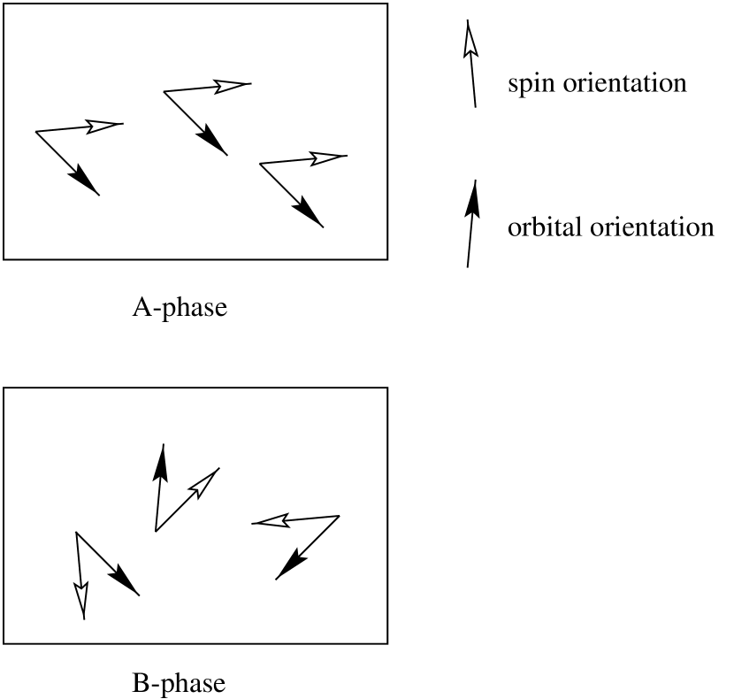
Figure 22: Depiction of the A- and B- phases of ³He. In the A-phase, the spin orientations of all the Cooper pairs are parallel and so are the orbital orientations. In the B-phase, the relative orientation of the spin and orbital orientations are fixed in all the Cooper pairs but neither the spin nor the orbital orientations of the various Cooper pairs are aligned.

In the B-phase, neither the orbital angular momenta nor the spin directions of the different Cooper pairs are aligned. But the angle between the direction of the angular momenta and the spin direction is fixed throughout the sample. Hence in the B-phase, independent rotations of the orbital angular momenta and of spin are no longer symmetries. However, a simultaneous rotation of both orbital angular momenta and spin remains an unbroken symmetry. In other words, a diagonal subgroup of $SO(3)_{S}\times SO(3)_{L}$ remains unbroken. Therefore, in the B-phase the order parameter is written as:

$$A_{\alpha i}=3^{-1/2}e^{i\phi}R_{\alpha i}({\hat{n}},\theta)$$ (245)

where, $\phi$ is a phase and the $3\times 3$ matrix $R_{\alpha i}$ describes relative rotations of the spin and orbital degrees of freedom about an axis ${\hat{n}}$ and by angle $\theta$. The symmetry breaking pattern is:

$$G\rightarrow SO(3)_{L_{3}+S_{3}}\ .$$ (246)

This symmetry breaking resembles the chiral symmetry breaking transition studied in QCD (with two flavors of quarks) and may be useful for experimentally investigating phenomenon such as the formation of “disoriented chiral condensates” [24]. The B-phase does not resemble the electroweak model and hence we will not discuss it any further. We shall also not discuss the various other phases of ³He (for example, the ${\rm A}_{1}$ phase) which are known to occur. (For a useful chart of the phases, see Sec. 6.2 of Ref. [133].)

In addition to the continuous symmetries, there are a number of discrete symmetries that arise in the phases of ³He. These are important for the classification of topological defects in ³He. A description may be found in [112].

11.2 Z-string analog in ³He

Clearly the A-phase closely resembles the electroweak symmetry breaking because of the mixing of the generator of the non-Abelian group ($SO(3)_{L}$) and the Abelian group ($U(1)_{N}$). The orbital part of the order parameter is responsible for this pattern of symmetry breaking and hence $\psi_{i}$ plays the role of the electroweak Higgs field $\Phi$. The connection, however, is indirect since $\psi_{i}$ is a complex 3 vector while $\Phi$ is a complex doublet. The idea is that the ³He-A real vector

$${\hat{l}}_{HeA}=i{{{\vec{\psi}}\times{{\vec{\psi}}^{{\dagger}}}}\over{{\vec{\psi}}^{{\dagger}}{\vec{\psi}}}}={\hat{m}}\times{\hat{n}}$$ (247)

is analogous to the electroweak real vector

$${\hat{l}}_{ew}=-{{\Phi^{{\dagger}}{\vec{\tau}}\Phi}\over{\Phi^{{\dagger}}{\vec{\tau}}\Phi}}\ .$$ (248)

The electroweak Z-string is a non-topological solution for which the Higgs field configuration is:

$$\Phi={\eta\over{\sqrt{2}}}f(r)e^{i\varphi}\pmatrix{0\cr 1\cr}\ .$$ (249)

For this configuration ${\hat{l}}_{ew}={\hat{z}}$.

The vacuum manifold $M_{A}$ of ³He-A has

$$\pi_{1}(M_{A})=Z_{4}$$ (250)

and hence there are topological $Z_{4}$ vortices in ³He-A. The vortices occur in classes labeled by $n=\pm 1/2,1$. The vortices with $n$ equal to an even integer are topologically equivalent to the vacuum. The non-trivial topological vortices (labeled by $n=\pm 1/2,1$) cannot be the equivalent of the non-topological Z-string. However, the topologically trivial $n=-2$ vortex is also seen in ³He-A. The order parameter for this vortex is:

$$A_{\alpha j}(\rho,\varphi)=\Delta_{0}\hat{z}_{\alpha}[\ e^{in\varphi}f_{1}(\rho)(\hat{x}_{j}+i\hat{y}_{j})+\ e^{i(n+2)\varphi}f_{2}(\rho)(\hat{x}_{j}-i\hat{y}_{j})]~{}~{}.$$ (251)

where $f_{1}(\rho)$ and $f_{2}(\rho)$ are two profile functions with $f_{1}(\infty)=1$, $f_{2}(\infty)=0$, $f_{1}(0)=0$ and $f_{2}(0)$ depending on $n$. In correspondence with the electroweak Z-string, the $n=2$ vortex has ${\hat{l}}_{HeA}={\hat{z}}$. However, the order parameter need not vanish at the center of the vortex for certain members of the $n=2$ class of vortices. For example, with $n=-2$, we may have $f_{2}(0)\neq 0$.

The $n=2$ vortex is not topological and can be continuously deformed into the vacuum manifold. The configuration at the terminus of the $n=2$ vortex is called the hedgehog or monopole ${\hat{l}}_{HeA}={\hat{r}}$ (the radial unit vector). This texture is the direct analog of the electroweak magnetic monopole (${\hat{l}}_{ew}={\hat{r}}$) at the terminus of a Z-string.

The $n=2$ discontinuous vortex is unstable but even so has been observed in ³He. In the laboratory, the rotation of the sample stabilizes the $n=2$ vortex. This seems to be closely analogous to the result of Garriga and Montes [47] who find that electroweak strings can be stabilized by external magnetic fields (Sec. 7.3).

Before proceeding further, it is prudent to remind ourselves of some important differences between the (bosonic sector of the) GSW model and ³He. The symmetries in ³He are all global whereas the symmetries in the GSW model are all local. So the $n=2$ discontinuous vortex is like a global analog of the Z-string. Another important difference is in the discrete symmetries in the two systems. The symmetry structure of the GSW model is really $[SU(2)\times U(1)]/Z_{2}$ since the $Z_{2}$ elements ${\bf 1}$ and $-{\bf 1}$ which form the center of $SU(2)$ also occur in $U(1)$. On the contrary, the symmetry group of ³He-A has a multiplicative $Z_{2}$ factor which gives rise to the non-trivial topology of the vacuum manifold.

It is important to note that we cannot expect ³He to provide an exact replica of the GSW model. However, the similar structures of the two systems means that certain issues can be experimentally addressed in the ³He context while they are far beyond the reach of current particle physics experiments. An issue of this kind is the baryon number anomaly in the GSW model and the anomalous generation of momentum in ³He.

As described in Sec. 8, there are fermionic zero modes on the Z-string and an electric field applied along the Z-string leads to the anomalous production of baryon number. What is the corresponding analog in ³He? At first sight, ³He does not have the non-Abelian gauge fields that the electroweak string has and so it seems that the analogy is doomed. But this is not true. The point is that the physics of fermionic zero modes has to do with the dynamics of fermions on the fixed background of the Z-string. Likewise, in ³He we can be interested in the dynamics of quasiparticles in the fixed background of the $n=2$ vortex. As far as the interaction of quasiparticles with the order parameter background is concerned, one can think of the ³He-A vortex as being due to a to a (fictitious) gauge field ${{Z^{\prime}}^{\mu}}$. Then the interaction of quasiparticles with the order parameter is of the form $j_{\mu}{{Z^{\prime}}^{\mu}}$ which is exactly analogous to the interaction of quarks and leptons with the Z-boson. Just as in the electroweak case, the ³He quasiparticles have zero modes on the vortex. In close analogy with the scenario where the motion of a superconducting string through an external magnetic field leads to currents along the string (Sec. 9.4), the velocity of the ³He vortex through the superfluid leads to an anomalous flow of quasiparticles but this time in the direction perpendicular to the vortex. This flow causes an extra force on the vortex as it moves through the superfluid that can be monitored experimentally. Such a force was measured in the Manchester experiment [20, 131] and is in excellent agreement with theoretical predictions. Hence the Manchester experiment verifies the anomalous production of quasiparticle momentum on moving vortices and the corresponding production of baryon number on electroweak strings moving through a magnetic field.

12 Concluding remarks and open problems

Quantum field theory has been very successful in describing particle physics. Yet the successes have mostly been relegated to perturbative phenomena. A more spectacular level of success will be achieved when our field theoretic description of particle physics is confirmed at the non-perturbative level. The first non-perturbative objects that are likely to be encountered in this quest are topological defects and their close cousins that we have described in this review.

The search for topological defects can be conducted in accelerator experiments or in the cosmological realm via astronomical surveys. These searches are complementary - only supermassive topological defects can be evident in astronomical surveys, while only the lightest defects can potentially be produced in accelerators. Foreseeable accelerator experiments give us access only to topological defects at the electroweak symmetry breaking scale. So it is very important to understand the defects present in the standard electroweak model and all its viable extensions. One may hope that the structure of defects will yield important clues about the underlying symmetry of the standard model.

With this hope, we have described wide classes of defects present in field theories. These defects are not all topological and this is relevant to the standard electroweak model which also lacks the non-trivial topology needed to contain topological defects. The absence of topology in the model means that the defect solutions cannot be enumerated in topological terms and neither can their stability be guaranteed. We have described, however, how the existence of defect solutions may still be derived by examining the topological defects occurring in subspaces of the model. The electroweak defects can be thought of as being topological defects that are embedded in the electroweak model.

The issue of stability of the defect solution is yet more involved and has not yet been fully resolved in the presence of fermions. That the electroweak Z-string is stable for large $\theta_{w}$ (within the bosonic sector) was inspired by the discovery of semilocal strings and their stability properties. The explicit stability analysis of the electroweak string marks out the region of parameter space in which the Z-string is stable. Then it is clear that the Z-string is unstable for the parameters of the standard model. In certain viable extensions of the standard model and under some external conditions (such as an external magnetic field), the standard electroweak Z-string can still be stable.

Even if the Z-string is unstable, it is possible that the lifetime of segments of string is long enough so that they can be observed in accelerators. This possibility was discussed in the first paper on the subject by Nambu [94]. The discovery of Z-string segments would truly be historic since it would confirm the existence of magnetic monopoles in particle physics. However, the rate of formation of Z-string segments and their lifetime has not yet been studied in detail. Some of the difficulties in this problem lie quite deep since they involve the connection of perturbative particle physics to the non-perturbative solitonic features. Additionally, the influence of fermions on electroweak strings needs further investigation.

Electroweak strings may play a cosmological role in the genesis of matter over antimatter as is evident since configurations of electroweak string have properties that are similar to the electroweak sphaleron. The challenge here is to determine the number density of electroweak strings formed during the electroweak phase transition and their decay rate. Note that the formation of topological strings has been under constant examination over the last two decades and only now, with some experimental input, are we beginning to understand their formation. The cosmological formation of electroweak defects has not been addressed with as much vigour. Recently though, there have been spurts of activity in this area, with lattice calculations beginning to shed interesting insight [27]. It is very likely that further lattice results will be able to give quantitative information about the formation of electroweak strings at the electroweak phase transition.

While particle physics experiments to detect electroweak strings are quite distant, experiments in condensed matter systems to study topological defects are becoming more feasible and can be used to test theoretical ideas that are relevant to both particle physics and condensed matter physics. Already there are experiments that test theories of the formation of topological vortices. We can also expect that condensed matter experiments might some day test the formation of defects that are not topological. The experiments on He³ are most relevant in this regard since it contains close analogs of electroweak strings. Furthermore, ideas relating to the behaviour of fermions in the background of electroweak strings can also be tested in the realm of He³. This makes for exciting physics in the years to come which will stimulate the growth of particle physics, cosmology and both, theoretical and experimental, condensed matter physics.

13 Acknowledgements

We are grateful to G. Volovik for very useful comments on section 11, to M. Groves and W. Perkins for an early draft of their paper, and to M. Hindmarsh for the sphaleron figures in section 10. AA thanks K. Kuijken and L. Perivolaropoulos for help with some of the figures in sections 2 and 3, and J. Urrestilla for pointing out several typos in an earlier draft.

This work was supported by a NATO Collaborative Research Grant CRG 951301, and our travel was also partially supported by NSF grants PHY-9309364 (AA), as well as by UPV grant UPV 063.310-EB187/98 and CICYT grant AEN-93-0435. TV was partially supported by the Department of Energy, USA. TV thanks the University of the Basque Country, and AA thanks Case Western Reserve University, Pierre Van Baal and Leiden University for their hospitality.

References

- [1]
- [2] E. Abraham, Nucl. Phys. B399 (1993) 197.
- [3] A.A. Abrikosov, Sov. Phys. JETP 5 (1957) 1174.
- [4] A. Achúcarro, J. Borrill and A. R. Liddle, Phys. Rev. D57 (1998) 3742.
- [5] A. Achúcarro, J. Borrill and A. R. Liddle, Phys. Rev. Lett. 82 (1999) 3742.
- [6] A. Achúcarro, J. Borrill and A. R. Liddle, Physica B255 (1998) 116.
- [7] A. Achúcarro, R. Gregory, J. A. Harvey and K. Kuijken, Phys. Rev. Lett. 72 (1994) 3646.
- [8] A. Achúcarro, K. Kuijken, L. Perivolaropoulos and T. Vachaspati, Nucl. Phys. B388 (1992) 435.
- [9] S. Adler, Phys. Rev. 177 (1969) 2426.
- [10] B. Allen, R.R. Caldwell, S. Dodelson, L. Knox, E.P.S. Shellard and A. Stebbins, Phys. Rev. Lett. 79 (1997) 2624; U.-L. Pen, U. Seljak and N. Turok, Phys. Rev. Lett. 79 (1997) 1611; A. Albrecht, R. A. Battye and J. Robinson, Phys. Rev. Lett. 79 (1997) 4736; A. Albrecht, R. A. Battye and J. Robinson, Report astro-ph/9711121.
- [11] J. Ambjørn and P. Olesen, Nucl. Phys. B315 (1989) 606; Nucl. Phys. B330 (1990) 193.
- [12] J. Ambjørn and P. Olesen, Int. J. Mod. Phys. A5 (1990) 4525.
- [13] M. Axenides, A. Johansen, H. B. Nielsen and O. Tornkvist, Nucl. Phys.B474 (1996) 3.
- [14] M. Barriola, Phys. Rev. D51 (1995) 300.
- [15] M. Barriola, T. Vachaspati and M. Bucher, Phys. Rev. D50 (1994) 2819.
- [16] M. Barriola and A. Vilenkin, Phys. Rev. Lett. 63 (1989) 341.
- [17] J. S. Bell and R. Jackiw, Nuovo Cimento A60 (1969) 47.
- [18] K. Benson and M. Bucher, Nucl. Phys. B406 (1993) 355.
- [19] M. Berger and G. Field, J. Fluid Mech. 147 (1984) 133.
- [20] T.D.C. Bevan, A.J. Manninen, J.B. Cook, J.R. Hook, H.E. Hall, T. Vachaspati and G.E. Volovik, Nature, 386 (1997) 689.
- [21] G. Bimonte and G. Lozano, Phys. Rev. D50 (1994) 6046.
- [22] G. Bimonte and G. Lozano, Phys. Lett. B326 (1994) 270.
- [23] G. Bimonte and G. Lozano, Phys. Lett. B348 (1995) 457.
- [24] J. D. Bjorken, Acta Phys. Polon. B28 (1997) 2773.
- [25] E. B. Bogomolnyi, Sov. J. Nucl. Phys. 24 (1976) 449 [Yad. Phys. 24 (1976) 861]; reprinted in [105].
- [26] I. Burlachkov and N.B. Kopnin, Sov. Phys. JETP 65 (1987) 630.
- [27] M. N. Chernodub, JETP Lett. 66 (1997) 605; M.N. Chernodub, F.V. Gubarev, E.-M. Ilgenfritz and A. Schiller, Nucl. Phys. Proc. Suppl. 73 (1999) 671. M. N. Chernodub, F. V. Gubarev, E.-M. Ilgenfritz and A. Schiller, Phys. Lett. B443 (1998) 244; M. N. Chernodub, F. V. Gubarev, E.-M. Ilgenfritz and A. Schiller, Phys.Lett. B434 (1998) 83; M. N. Chernodub, F. V. Gubarev and E.-M. Ilgenfritz, Phys.Lett. B424 (1998) 106.
- [28] T. P. Cheng and L. F. Li, “Gauge Theory of Elementary Particle Physics”, Oxford University Press (1991).
- [29] Y.M. Cho and D. Maison, Phys. Lett. 391B (1997) 360.
- [30] S. Coleman, “Aspects of Symmetry” (Cambridge University Press, Cambridge, 1985).
- [31] S. Coleman, Nucl. Phys. B262 (1985) 263.
- [32] E. J. Copeland, E. W. Kolb and K. Lee, Phys. Rev. D38 (1988) 3023.
- [33] S. C. Davis, A–C. Davis and M. Trodden, Phys. Rev. D57 (1998) 5184.
- [34] A–C. Davis and N. Lepora, Phys. Rev. D52 (1995) 7265.
- [35] A–C. Davis, A.P. Martin and N. Ganoulis, Nucl. Phys. B419 (1994) 323.
- [36] G. Dvali and G. Senjanović, Phys. Lett. B331 (1994) 63.
- [37] M. A. Earnshaw and M. James, Phys. Rev. D48 (1993) 5818.
- [38] M. A. Earnshaw and W. B. Perkins, Phys. Lett. B328 (1994) 337.
- [39] M.B. Einhorn and R. Savit, Phys. Lett. B77 (1981) 295; V. Soni, Phys. Lett. B93 (1980) 101; K. Huang and R. Tipton, Phys. Rev. D23 (1981) 3050; J.M. Gipson and C.H. Tze, Nucl. Phys. B183 (1981) 524.
- [40] K. Enqvist and P. Olesen, Phys. Lett. B319 (1993) 178.
- [41] A. Everett, Phys. Rev. D24 (1981) 858.
- [42] E. Farhi, J. Goldstone, S. Gutman, K. Rajagopal and R. Singleton, Phys. Rev. D51 (1995) 4561.
- [43] E. Farhi, J. Goldstone, A. Lue and K. Rajagopalan, Phys. Rev. D54 (1996) 5336.
- [44] R. Friedberg, T. D. Lee and A. Sirlin, Phys. Rev. D13 (1976) 2739.
- [45] K. Fujii, S. Otsuki and F. Toyoda, Prog. Theor. Phys. 81 (1989) 462.
- [46] N. Ganoulis, Phys. Lett. B298 (1993) 63.
- [47] J. Garriga and X. Montes, Phys. Rev. Lett. 75 (1995) 2268.
- [48] J. Garriga and T. Vachaspati, Nucl. Phys. B438 (1995) 161.
- [49] G.W. Gibbons, M. Ortiz, F. Ruiz-Ruiz and T. Samols, Nucl. Phys. B385 (1992) 127.
- [50] G. Glashow, Nucl. Phys 22 (1961) 579; S. Weinberg, Phys. Rev. Lett. 19 (1967) 1264; A. Salam, in “Elementary particle physics” (Nobel Symp. no. 8), ed. N. Svartholm, Almqvist and Wilsell, Stockholm 1968.
- [51] A. Goldhaber, Phys. Rev. Lett. 63 (1989) 719.
- [52] J. Goldstone and R. Jackiw, Phys. Rev. D11 (1975) 1486.
- [53] M. Goodband and M. Hindmarsh, Phys. Rev. D52 (1995) 4621.
- [54] M. Goodband and M. Hindmarsh, Phys. Lett. B363 (1995) 58.
- [55] M. Groves and W. Perkins, (private communication, 1999).
- [56] M. Hindmarsh, Phys. Rev. Lett. 68 (1992) 1263.
- [57] M. Hindmarsh, Nucl. Phys. B392 (1993) 461.
- [58] M. Hindmarsh, R. Holman, T.W. Kephart and T. Vachaspati, Nucl. Phys. B404 (1993) 794.
- [59] M. Hindmarsh, in the Proceedings of the NATO Workshop on “Electroweak Physics and the Early Universe”, eds. J. C. Romão and F. Freire, Sintra, Portugal (1994); Series B: Physics Vol. 338, Plenum Press, New York (1994).
- [60] M. Hindmarsh and M. James, Phys. Rev. D49 (1994) 6109.
- [61] R. Holman, S. Hsu, T. Vachaspati and R. Watkins, Phys. Rev. D46 (1992) 5352.
- [62] G. ’t Hooft, Nucl. Phys. B79 (1974) 276; A. M. Polyakov, JETP Lett. 20 (1974) 194.
- [63] J. D. Jackson, “Classical Electrodynamics”, John Wiley & Sons, 1975.
- [64] R. Jackiw and P. Rossi, Nucl. Phys. B190 (1981) 681.
- [65] A. Jaffe and C. Taubes, “Vortices and monopoles”, Progress in Physics 2 (Birkhäuser, Basel, 1980); C.H. Taubes, Comm. Math. Phys. 72 (1980) 277; ibid. 75 (1980) 207.
- [66] M. James, Phys. Lett. B334 (1994) 121.
- [67] M. James, L. Perivolaropoulos and T. Vachaspati, Phys. Rev. D46 (1992) R5232; Nucl. Phys. B395 (1993) 534.
- [68] B. Julia and A. Zee, Phys. Rev. D11 (1975) 2227.
- [69] See, e.g. B. Kastening, Report hep-ph/9307224.
- [70] T. W. Kephart (1998) unpublished.
- [71] T. W. Kephart and T. Vachaspati, Phys. Lett. B388 (1996) 481.
- [72] T. W. B. Kibble, J. Phys. A9 (1976) 1387.
- [73] F. Klinkhamer, Nucl. Phys. B535 (1998) 233.
- [74] F. R. Klinkhamer and N. S. Manton, Phys. Rev. D30 (1984) 2212.
- [75] F. R. Klinkhamer and P. Olesen, Nuc. Phys. B422 (1994) 227.
- [76] F. Klinkhamer, C. Rupp, Nucl. Phys B495 (1997) 172.
- [77] S. Kono and S. G. Naculich, Proc. of PASCOS/HOPKINS 1995, Baltimore, (1995); Report hep-ph/9507350.
- [78] R. Leese, Phys. Rev. D46 (1992) 4677.
- [79] R. Leese and T.M. Samols, Nucl. Phys. B396 (1993) 639.
- [80] N. Lepora and A–C. Davis, Phys. Rev. D58 (1998) 125027; ibid Phys. Rev. D58 (1998) 125028.
- [81] N. Lepora, T.W.B. Kibble, Phys. Rev. D59 (1999) 125019.
- [82] N. Lepora, T.W.B. Kibble, JHEP 9904 (1999) 027.
- [83] M. Liu, Physica 109/110B+C (1982) 1615 (Proceedings of the 16th International Conference on Low Temperature Physics, LT-16).
- [84] H. Liu and T. Vachaspati, Nuc. Phys. B470 (1996) 176.
- [85] H-K Lo, Phys. Rev. D51 (1995) 802.
- [86] S. W. MacDowell and O. Tornkvist, in the proceedings of the “Gürsey Memorial Conference on Strings and Symmetries”, Istanbul, Turkey (1994).
- [87] S. W. MacDowell and O. Tornkvist, Mod. Phys. Lett. A10 (1995) 1065.
- [88] K. Maki, Physics 90B (1977) 84.
- [89] N. S. Manton, Phys. Lett. 110B (1982) 54.
- [90] N. S. Manton, Phys. Rev. D28 (1983) 2019.
- [91] N. S. Manton, Ann. of Phys. 159 (1985) 220.
- [92] J. M. Moreno, D. H. Oaknin and M. Quirós, Phys. Lett. B347 (1995) 332.
- [93] S. Naculich, Phys. Rev. Lett. 75 (1995) 998.
- [94] Y. Nambu, Nucl. Phys. B130 (1977) 505.
- [95] See, for instance, Formation and Interactions of Topological Defects, NATO-ASI series B, Physics, vol. 349, eds. A.C. Davis and R. Brandenberger, Plenum Press 1995.
- [96] C. Bäuerle, Yu.M. Bunkov, S.N. Fisher, H. Godfrin and G.R. Pickett, Nature 382 (1996) 332; V.M.H. Ruutu, V.B. Eltsov, A.J. Gill, T.W.B. Kibble, M. Krusius, Yu.G. Makhlin, B. Plaçais, G.E. Volovik and Wen Xu, Nature 382 (1996) 334.
- [97] H. B. Nielsen and P. Olesen, Nucl. Phys. B61 (1973) 45.
- [98] M. Nagasawa and J. Yokoyama, Phys. Rev. Lett. 77 (1996) 2166.
- [99] W. B. Perkins, Phys. Rev. D17 (1993) 5224.
- [100] L. Perivolaropoulos, Phys. Rev. D48 (1993) 5961.
- [101] L. Perivolaropoulos, Phys. Rev. D50 (1994) 962.
- [102] W.B. Perkins, L. Perivolaropoulos, A.C. Davis, R.H. Brandenberger and A. Matheson, Nucl. Phys. B353 (1991) 237.
- [103] J. Preskill, Phys. Rev. D46 (1992) 4218.
- [104] J. Preskill and A. Vilenkin, Phys. Rev. D47 (1992) 4218.
- [105] “Solitons and Particles”, eds. C. Rebbi and G. Soliani, World Scientific (Singapore, 1984).
- [106] P. Goddard and D. Olive, Rep. Prog. Phys. 41 (1978) 1357-1437; T. W. B. Kibble, Phys. Rep. 67 (1980) 183; A. Vilenkin Phys. Rep. 121 (1985) 1; J. Preskill, “Vortices and Monopoles”, lectures presented at the 1985 Les Houches Summer School, Les Houches France; A. Vilenkin and E. P. S. Shellard, “Cosmic Strings and Other Topological Defects”, Cambridge University Press, Cambridge (1994); R. Brandenberger, Int. J. Mod. Phys. A9 (1994) 2117; M. Hindmarsh and T. W. B. Kibble, Rep. Prog. Phys. 58 (1995) 477.
- [107] A. Robergé, Ph. D. thesis, University of British Columbia (1989).
- [108] G. Rosen, J. Math. Phys. 9 (1968) 996; 9 (1968) 999.
- [109] P. J. Ruback, Nucl. Phys. B296 (1988) 669.
- [110] P. Saffin and E. Copeland, Phys. Rev. D56 (1997) 1215; E. Copeland and P. Saffin, Phys. Rev. D54 (1996) 6088.
- [111] T. M. Samols, Comm. Math. Phys. 145 (1992) 149.
- [112] M. M. Salomaa and G. E. Volovik, Rev. Mod. Phys. 59 (1987) 533.
- [113] G. D. Starkman and T. Vachaspati, Phys. Rev. D53 (1996) 6711.
- [114] C. Taubes, Comm. Math. Phys. 86 (1982) 299.
- [115] T.N. Tomaras, Report hep-ph/9707236, to appear in the Proceedings of the XXXII-th Rencontres de Moriond, ”Electroweak Interactions and Unified Theories”, Les Arcs, France (1997).
- [116] O. Tornkvist, Report no. hep-ph/9805255.
- [117] T. Vachaspati, Phys. Lett. B265 (1991) 258.
- [118] T. Vachaspati, Phys. Rev. Lett. 68 (1992) 1977; 69 (1992) 216(E).
- [119] T. Vachaspati, Nucl. Phys. B397 (1993) 648.
- [120] T. Vachaspati, in the Proceedings of the NATO Workshop on “Electroweak Physics and the Early Universe”, eds. J. C. Romão and F. Freire, Sintra, Portugal (1994); Series B: Physics Vol. 338, Plenum Press, New York (1994).
- [121] T. Vachaspati, Nucl. Phys. B439 (1995) 79.
- [122] T. Vachaspati and A. Achúcarro, Phys. Rev. D44, 3067 (1991).
- [123] T. Vachaspati and M. Barriola, Phys. Rev. Lett. 69 (1992) 1867.
- [124] T. Vachaspati and G. B. Field, Phys. Rev. Lett. 73 (1994) 373; 74 (1995) Errata.
- [125] T. Vachaspati and A. Vilenkin, Phys. Rev. D30 (1984) 2036.
- [126] T. Vachaspati and R. Watkins, Phys. Lett. B318 (1993) 163.
- [127] P. di Vecchia and S. Ferrara, Nucl. Phys. B130 (1977) 93.
- [128] H. de Vega, Phys. Rev. D18 (1978) 2932.
- [129] G.E. Volovik, Sov. Phys. Usp. 27 (1984) 363.
- [130] G. E. Volovik, “Exotic Properties of Superfluid 3He” (World Scientific, Singapore, 1992).
- [131] G. E. Volovik, to be published in the proceedings of “Symposium on Quantum Phenomena at Low Temperatures”, Lammi (Finland), 1998; cond-mat/9802091.
- [132] G. E. Volovik and T. Vachaspati, Int. J. Mod. Phys. B10 (1996) 471.
- [133] D. Volhardt and P. Wolfle, “The Superfluid Phases of 3He” (Taylor and Francis, London, 1990).
- [134] E. Witten, Phys. Lett. B86 (1979) 283.
- [135] W. H. Zurek, Nature 317 (1985) 505.