DESY 99-021
April 1999
NEUTRINO MIXING AND THE PATTERN
OF SUPERSYMMETRY BREAKING

Abstract

We study the implications of a large $\nu_{\mu}$-$\nu_{\tau}$ mixing angle on lepton flavour violating radiative transitions in supersymmetric extensions of the standard model. The transition rates are calculated to leading order in $\epsilon$, the parameter which characterizes the flavour mixing. The uncertainty of the predicted rates is discussed in detail. For models with modular invariance the branching ratio $BR(\mu\rightarrow e\gamma)$ mostly exceeds the experimental upper limit. In models with radiatively induced flavour mixing the predicted range includes the upper limit, if the Yukawa couplings in the lepton sector are large, as favoured by Yukawa coupling unification.

In connection with the recently reported atmospheric neutrino anomaly [1] the possibility of neutrino oscillations associated with a large $\nu_{\mu}$-$\nu_{\tau}$ mixing angle has received wide attention. The smallness of the corresponding neutrino masses can be accounted for by the seesaw mechanism [2], which leads to the prediction of heavy Majorana neutrinos with masses close to the unification scale $\Lambda_{GUT}$.

A large $\nu_{\mu}$-$\nu_{\tau}$ mixing angle as well as the mass hierarchies of quarks and charged leptons can be naturally explained by the Frogatt-Nielsen mechanism based on a U(1)_F family symmetry [3] together with a nonparallel family structure of chiral charges [4, 5, 6]. Depending on the family symmetry, such models can also explain the magnitude of the observed baryon asymmetry [7]. The expected phenomenology of neutrino oscillations depends on details of the model [8, 9].

The large hierarchy between the electroweak scale and the unification scale, and now also the mass scale of the heavy Majorana neutrinos, motivates supersymmetric extensions of the standard model [10]. This is further supported by the observed unification of gauge couplings. The least understood aspect of the supersymmetric standard model is the mechanism of supersymmetry breaking and the corresponding pattern of soft supersymmetry breaking masses and couplings.

It is well known that constraints from rare processes severely restrict the allowed pattern of supersymmetry breaking [10]. In this paper we therefore study lepton flavour changing radiative transition [11]. In the standard scenario with universal soft breaking terms at the GUT scale, radiative corrections induce flavour mixing at the electroweak scale. These effects can be important in the case of large Yukawa couplings [12, 13]. Following [14] we shall contrast these minimal models with the interesting class of models possessing modular invariance [15].

In this paper we shall restrict our discussion to one particular example with SU(5)$\otimes$U(1)_F symmetry [4, 7]. However, the results will be presented in such a form that they can easily be applied to other examples of lepton mass matrices [16]. We shall also address the uncertainty of the predicted lepton flavour changing transition rates.

We consider the leptonic sector of the supersymmetric standard model with right-handed neutrinos, which is described by the superpotential

$$W=h_{eij}\hat{E}^{c}_{i}\hat{L}_{j}\hat{H}_{1}+h_{\nu ij}\hat{N}^{c}_{i}\hat{L}_{j}\hat{H}_{2}+\mu\hat{H}_{1}\hat{H}_{2}+\frac{1}{2}h_{rij}\hat{N}^{c}_{i}\hat{N}^{c}_{j}\hat{R}\;.$$ (1)

Here $i,j=1\ldots 3$ are generation indices, and the superfields $\hat{E}^{c}$, $\hat{L}=(\hat{N},\hat{E})$, $\hat{N}^{c}$ contain the leptons $e_{R}^{c}$, $(\nu_{L},e_{L})$, $\nu_{R}^{c}$, respectively. The expectation values of the Higgs multiplets $H_{1}$ and $H_{2}$ generate ordinary Dirac masses of quarks and leptons, and the expectation value of the singlet Higgs field $R$ yields the Majorana mass matrix of the right-handed neutrinos.

In the following discussion the scalar masses will play a crucial role. They are determined by the superpotential and the soft breaking terms,

$${\cal{L}}_{soft}=-{\widetilde{m}}^{2}_{lij}L^{\dagger}_{i}L_{j}-{\widetilde{m}}^{2\dagger}_{eij}E^{c\dagger}_{i}E^{c}_{j}+A_{eij}E^{c}_{i}L_{j}H_{1}+c.c.+\ldots\;,$$ (2)

where $L=(N_{L},E_{L})$ and $E^{c}\equiv E_{R}^{*}$ denote the scalar partners of $(\nu_{L},e_{L})$ and $e_{R}^{c}$, respectively. Using the seesaw mechanism to explain the smallness of neutrino masses, we assume that the right-handed neutrino masses $M_{i}$ are much larger than the Fermi scale $v$. One then easily verifies that all mixing effects on light scalar masses caused by the right-handed neutrinos and their scalar partners are suppressed by ${\cal O}(v/M_{i})$, and therefore negligible.

The mass terms of the light scalar leptons are given by

$${\cal{L}}_{M}=-E^{\dagger}{\widetilde{M}_{e}}^{2}E-N_{L}^{\dagger}{\widetilde{m}_{l}}^{2}N_{L}\;,$$ (3)

where $\widetilde{M}_{e}^{2}$ is the mass matrix of the charged scalar fields $E=(E_{L},E_{R})$,

$${\widetilde{M}_{e}}^{2}\ \equiv\ \left(\begin{array}[]{ll}{\widetilde{M}_{L}}^{2}&{\widetilde{M}_{LR}}^{2}\\[4.30554pt] {\widetilde{M}_{RL}}^{2}&{\widetilde{M}_{R}}^{2}\\[4.30554pt] \end{array}\right)\ =\ \left(\begin{array}[]{ll}{\widetilde{m}_{l}}^{2}+v_{1}^{2}h_{e}^{\dagger}h_{e}&v_{1}A_{e}^{\dagger}+\mu v_{2}h_{e}^{\dagger}\\[4.30554pt] v_{1}A_{e}+\mu v_{2}h_{e}&{\widetilde{m}_{e}}^{2}+v_{1}^{2}h_{e}h_{e}^{\dagger}\\[4.30554pt] \end{array}\right)\;.$$ (4)

According to the Frogatt-Nielsen mechanism [3] the hierarchies among the various Yukawa couplings are related to a spontaneously broken U(1)_F generation symmetry. The Yukawa couplings arise from non-renormalizable interactions after a gauge singlet field $\Phi$ acquires a vacuum expectation value,

$$h_{ij}=g_{ij}\left({\left\langle\Phi\right\rangle\over\Lambda}\right)^{Q_{i}+Q_{j}}\;.$$ (5)

Here $g_{ij}$ are couplings ${\cal O}(1)$ and $Q_{i}$ are the U(1) charges of the various superfields with $Q_{\Phi}=-1$. The interaction scale $\Lambda$ is expected to be very large, $\Lambda>\Lambda_{GUT}$, and the phenomenology of quark and lepton mass matrices can be explained assuming

$$\left({\left\langle\Phi\right\rangle\over\Lambda}\right)^{2}\equiv\epsilon^{2}\simeq\left({m_{\mu}\over m_{\tau}}\right)^{2}\simeq{1\over 300}\;.$$ (6)

$\hat{\Phi}_{i}$	$\hat{E}^{c}_{3}$	$\hat{E}^{c}_{2}$	$\hat{E}^{c}_{1}$	$\hat{L}_{3}$	$\hat{L}_{2}$	$\hat{L}_{1}$	$\hat{N}^{c}_{3}$	$\hat{N}^{c}_{2}$	$\hat{N}^{c}_{1}$
$Q_{i}$	0	1	2	$a$	$a$	$a+1$	0	$1-a$	$2-a$

Table 1: Chiral charges for lepton superfields; a=0 or 1 [7].

The special feature of the two sets of charges $Q_{i}$ in table 1 is the non-parallel family structure. The assignment of the same charge to the lepton doublets of the second and third generation leads to a neutrino mass matrix of the form[4, 5],

$$m_{\nu_{ij}}\sim\epsilon^{a}\left(\begin{array}[]{ccc}\epsilon^{2}&\epsilon&\epsilon\\[4.30554pt] \epsilon&1&1\\[4.30554pt] \epsilon&1&1\end{array}\right){v^{2}\over\left\langle R\right\rangle}\;,$$ (7)

which can account for the large $\nu_{\mu}-\nu_{\tau}$ mixing angle. This form of the mass matrix is compatible with small and large mixing angle solutions of the solar neutrino problem. The Yukawa matrices which yield the Dirac masses of neutrinos and charged leptons have the general structure,

$$h_{e}\sim\ \epsilon^{a}\ \left(\begin{array}[]{ccc}\epsilon^{3}&\epsilon^{2}&\epsilon^{2}\\[4.30554pt] \epsilon^{2}&\epsilon&\epsilon\\[4.30554pt] \epsilon&1&1\end{array}\right)\;,\quad h_{\nu}\sim\ \epsilon^{a}\ \left(\begin{array}[]{ccc}\epsilon^{3-a}&\epsilon^{2-a}&\epsilon^{2-a}\\[4.30554pt] \epsilon^{2-a}&\epsilon^{1-a}&\epsilon^{1-a}\\[4.30554pt] \epsilon&1&1\end{array}\right)\;.$$ (8)

The Yukawa matrix for the right-handed neutrinos can always be chosen diagonal,

$$h_{r}\sim\ \left(\begin{array}[]{ccc}\epsilon^{4-2a}&0&0\\[4.30554pt] 0&\epsilon^{2-2a}&0\\[4.30554pt] 0&0&1\end{array}\right)\;.$$ (9)

The corresponding unitary transformation does not change the structure of $h_{\nu}$. In eqs. (7)-(9) factors ${\cal O}(1)$ have been omitted and we assume that there is no degeneracy in the right-handed neutrino mass matrix.

In models with gravity mediated supersymmetry breaking one usually assumes universal soft breaking terms at the GUT scale,

$${\widetilde{m}_{l}}^{2}={\widetilde{m}_{e}}^{2}=M^{2}1\!\!1\;,\quad A_{e}=h_{e}A\;,\quad A_{\nu}=h_{\nu}A\;.$$ (10)

Renormalization effects change these matrices significantly at lower scales. As a consequence the flavour structure in the scalar sector is different from the one in the fermionic sector. Integrating the renormalization group equations from the GUT scale, and taking the decoupling of the heavy neutrinos at their respective masses $M_{k}$ into account, one obtains at scales $\mu\ll M_{1}$,

$$\delta\widetilde{m}^{2}_{lij} \simeq -{1\over 8\pi^{2}}(3M^{2}+A^{2})h^{\dagger}_{\nu ik}\ln{\Lambda_{GUT}\over M_{k}}h_{\nu kj}\;,$$

$$\delta A_{eij} \simeq -{1\over 8\pi^{2}}A(h_{e}h^{\dagger}_{\nu})_{ik}\ln{\Lambda_{GUT}\over M_{k}}h_{\nu kj}\;.$$ (11)

In the following we shall discuss decay rates for lepton number changing radiative transitions to leading order in $\epsilon$ and we will not be able to discuss factors ${\cal O}(1)$. We therefore neglect terms $\sim\ln{\epsilon^{2}}$ which reflect the splitting between the heavy neutrino masses and evaluate $\ln(\Lambda_{GUT}/M_{k})$ for an average mass $\overline{M}=10^{12}$ GeV. In eqs. (DESY 99-021 April 1999 NEUTRINO MIXING AND THE PATTERN OF SUPERSYMMETRY BREAKING ) this yields the overall factor $\ln(\Lambda_{GUT}/\overline{M})\sim 10$. The flavour structure of the left-left scalar mass matrix is then identical to the one of the neutrino mass matrix,

$$\delta\widetilde{m}^{2}_{lij}\sim{1\over 8\pi^{2}}(3M^{2}+A^{2})\ln{\Lambda_{GUT}\over\overline{M}}\ \epsilon^{2a}\ \left(\begin{array}[]{ccc}\epsilon^{2}&\epsilon&\epsilon\\[4.30554pt] \epsilon&1&1\\[4.30554pt] \epsilon&1&1\end{array}\right)\;.$$ (12)

For the flavour changing left-right scalar mass matrix one obtains

$$v_{1}\delta A_{eij}\sim{1\over 8\pi^{2}}Am_{\tau}\ln{\Lambda_{GUT}\over\overline{M}}\ \epsilon^{2a}\ \left(\begin{array}[]{ccc}\epsilon^{3}&\epsilon^{2}&\epsilon^{2}\\[4.30554pt] \epsilon^{2}&\epsilon&\epsilon\\[4.30554pt] \epsilon&1&1\end{array}\right)\;.$$ (13)

For a wide class of supergravity models the possibilities of supersymmetry breaking can be parametrized by vacuum expectation values of moduli fields $T_{\alpha}$ and the dilaton field $S$ [17]. The structure of the soft breaking terms is determined by the modular weights of the various superfields. An interesting structure arises if the theory possesses both, modular invariance and a chiral U(1) symmetry. In this case the supersymmetry breaking scalar mass terms are directly related to the charges of the corresponding superfields [18],

$${\widetilde{m}}^{2}_{ij}=\left((1+B_{i}(\Theta_{\alpha}))\delta_{ij}+|Q_{i}-Q_{j}|C_{ij}(\Theta_{\alpha})\times\epsilon^{|Q_{i}-Q_{j}|}\right)M^{2}\;,$$ (14)

where the $\Theta_{\alpha}$ parametrize the direction of the goldstino in the moduli space. For pure dilaton breaking, $\Theta_{\alpha}=0$, one has $C_{ij}=0$ and the soft breaking terms are flavour diagonal. In the general case, instead, we get from eq. (14),

$${\widetilde{m}}^{2}_{l}\sim\ \left(\begin{array}[]{ccc}1&\epsilon&\epsilon\\[4.30554pt] \epsilon&1&0\\[4.30554pt] \epsilon&0&1\end{array}\right)\ M^{2}\;,\quad{\widetilde{m}}^{2}_{e}\sim\ \left(\begin{array}[]{ccc}1&\epsilon&\epsilon^{2}\\[4.30554pt] \epsilon&1&\epsilon\\[4.30554pt] \epsilon^{2}&\epsilon&1\end{array}\right)\ M^{2}\;.$$ (15)

Note, that the zeros in ${\widetilde{m}}^{2}_{l}$ occur since the lepton doublets of the second and the third family carry the same U(1)_F charge. The trilinear soft breaking terms are also affected by modular invariance [18]. The effect is to increase the branching ratio of lepton flavour violating processes. In order to obtain a lower bound, we shall take the trilinear soft breaking terms flavour diagonal and we shall only consider the effects of the lepton flavour changing scalar mass terms in the modular invariance case.

The scalar mass matrices (12), (13) and (15) are given in the weak eigenstate basis. In order to discuss the radiative transitions $\mu\rightarrow e\gamma$ and $\tau\rightarrow\mu\gamma$ we have to change to a mass eigenstate basis of the charged leptons. The Yukawa matrix $h_{e}$ can be diagonalized by a bi-unitary transformation, $U^{\dagger}h_{e}V=h_{e}^{D}$. To leading order in $\epsilon$ the matrices $U$ and $V$ are given by

$$U=\left(\begin{array}[]{ccc}1&a\epsilon&b\epsilon^{2}\\[4.30554pt] -a\epsilon&1&f\epsilon\\[4.30554pt] -b\epsilon^{2}&-f\epsilon&1\end{array}\right)\;,\quad V=\left(\begin{array}[]{ccc}1&(ca^{\prime}-sb^{\prime})\epsilon&(sa^{\prime}+cb^{\prime})\epsilon\\[4.30554pt] -a^{\prime}\epsilon&c&s\\[4.30554pt] -b^{\prime}\epsilon&-s&c\end{array}\right)\;,$$ (16)

where $c=\cos{\varphi}$ and $s=\sin{\varphi}$; $a,b,a^{\prime}$ and $b^{\prime}$ depend on the coefficients ${\cal O}(1)$ in $h_{e}$ which are not given in eq. (8). The scalar mass matrices transform as $V^{\dagger}\delta\widetilde{m}_{l}^{2}V$, $U^{\dagger}v_{1}A_{e}V$, $V^{\dagger}\widetilde{m}^{2}_{l}V$, $U^{\dagger}\widetilde{m}_{e}^{2}U$. One easily verifies that the form of the matrices given in eqs. (12), (13) and (15) is invariant under this transformation.

Given the Yukawa matrices and the scalar mass matrices it is straightforward to calculate the rates for radiative transitions. The transition $\mu\rightarrow e\gamma$ has the form

$${\cal M}_{\mu}=ie\bar{u}_{e}(p-q)\sigma_{\mu\nu}q^{\nu}(A_{L12}P_{L}+A_{R12}P_{R})u_{\mu}(p)\;,$$ (17)

where $P_{L}$ and $P_{R}$ are the projectors on states with left- and right-handed chirality, respectively. The corresponding branching ratio is given by

$$BR(\mu\rightarrow e\gamma)=384\pi^{3}\alpha{v^{4}\over m_{\mu}^{2}}(|A_{L12}|^{2}+|A_{R12}|^{2})\;,$$ (18)

where $v=(8G_{F}^{2})^{1/4}\simeq 174$ GeV is the Higgs vacuum expectation value.

At one-loop order the transition amplitudes for a left(right)-handed muon $A_{L(R)}^{(b)}$ and $A_{R}^{(w)}$ involve neutral and charged gauginos, respectively. Note, that the amplitude $A_{L}^{(w)}$ is suppressed by inverse powers of the heavy neutrino masses $M_{i}$. The radiative transition changes chirality. Amplitudes, where the chirality change is due to the gaugino require a left-right scalar transition and one or two scalar flavour changes (figs. (1.a)-(1.d)).

From eq. (4) and (10) one reads off,

$${\widetilde{M}_{RL}}^{2}=(A+\mu\tan{\beta})M_{e}\;,$$ (19)

where $\tan{\beta}=v_{2}/v_{1}$, and $M_{e}=h_{e}v_{1}$ is the charged lepton mass matrix. Amplitudes with chirality change of the external muon have one scalar flavour change to leading order in $\epsilon$ for neutral (fig. (1.e)) and charged (fig. (1.f)) gaugino.

Simple compact expressions can be given for the various transition amplitudes if one expands the scalar mass matrices around the dominant universal mass matrix $M1\!\!1$, i.e., $\widetilde{m}^{2}_{l}=M^{2}1\!\!1+\delta\widetilde{m}^{2}_{l}$, $\widetilde{M}^{2}_{L,R}=M^{2}1\!\!1+\delta\widetilde{M}^{2}_{L,R}$. For the bino ($b$) and chargino ($w^{-}$) contributions to the transition amplitude one obtains,

$$A^{(b)}_{L,R}={\alpha\over 4\pi\cos^{2}{\Theta_{W}}}\bar{A}^{(b)}_{L,R}\;,\quad A^{(w^{-})}_{R}={\alpha\over 8\pi\sin^{2}{\Theta_{W}}}\bar{A}^{(w)}_{R}\;,$$ (20)

where

$$\bar{A}^{(b)}_{L12} = Y_{L}Y_{R}m_{b}\left((\widetilde{M}_{RL}^{2})_{12}{\partial\over\partial M^{2}}+{1\over 2}(\delta\widetilde{M}_{R}^{2}\widetilde{M}_{RL}^{2}+\widetilde{M}_{RL}^{2}\delta\widetilde{M}_{L}^{2})_{12}{\partial^{2}\over\partial(M^{2})^{2}}\right.$$ (21)

$$\left.\hskip 56.9055pt+{1\over 3!}(\delta\widetilde{M}_{R}^{2}\widetilde{M}_{RL}^{2}\delta\widetilde{M}_{L}^{2})_{12}{\partial^{3}\over\partial(M^{2})^{3}}\right)F(m_{b}^{2},M^{2})$$

$$-Y_{R}^{2}m_{\mu}(\delta\widetilde{M}_{R}^{2})_{12}{\partial\over\partial M^{2}}G(m_{b}^{2},M^{2})+...\;,$$

$$\bar{A}^{(w)}_{R12} = -m_{\mu}(\delta\widetilde{m}_{l}^{2})_{12}{\partial\over\partial M^{2}}G(M^{2},m_{w}^{2})+...\;.$$ (22)

Here $m_{b}$, $m_{w}$ and $M$ are bino, charged wino and scalar masses, and $Y_{L}=-1/2$ and $Y_{R}=-1$ are the hypercharges of the lepton multiplets $l_{L}$ and $e_{R}$, respectively. The amplitude $A^{(b)}_{R}$ is obtained from $A^{(b)}_{L}$ by interchanging all subscripts $L$ and $R$. In eqs. (21) and (22) the dependence on the gaugino masses and the average scalar mass $M$ has been separated from the dependence on the lepton flavour beaking parameters. The functions $F(m^{2},M^{2})$ and $G(m^{2},M^{2})$ read

$$F(m^{2},M^{2}) = {M^{4}-m^{4}+2m^{2}M^{2}\ln{m^{2}\over M^{2}}\over(M^{2}-m^{2})^{3}}\;,$$ (23)

$$G(m^{2},M^{2}) = {M^{6}-6m^{2}M^{4}+3m^{4}M^{2}+2m^{6}-6m^{4}M^{2}\ln{m^{2}\over M^{2}}\over 6(m^{2}-M^{2})^{4}}\;.$$ (24)

The mixing between Higgsino and gaugino gives also a contribution to the leading order in $\epsilon$. The diagrams contributing to the amplitude are illustrated in fig.(1.g) and fig.(1.h)

and the corresponding amplitudes are given by

$$A^{(b,\tilde{h}_{0})}_{L,R}={\alpha\over 4\pi\cos^{2}{\Theta_{W}}}\bar{A}^{(b,\tilde{h}_{0})}_{L,R}\;,\quad A^{(w^{-},\tilde{h}^{-})}_{R}={\alpha\over 8\pi\sin^{2}{\Theta_{W}}}\bar{A}^{(w^{-},\tilde{h}^{-})}_{R}\;,$$ (25)

where

$$\bar{A}^{(b,\tilde{h}_{0})}_{R,L12} = Y_{L,R}m_{\mu}(\delta\widetilde{M}_{L,R}^{2})_{12}\left\{\frac{\mu^{2}+\tan\beta\mu m_{b}}{m_{b}^{2}-\mu^{2}}{\partial\over\partial M^{2}}F(\mu^{2},M^{2})+(\mu\leftrightarrow m_{b})\right\},$$ (26)

$$\bar{A}^{(w^{-},\tilde{h}^{-})}_{R12} = -m_{\mu}(\delta\widetilde{m}_{l}^{2})_{12}\left\{\frac{\mu^{2}+\tan\beta\mu m_{w}}{m_{w}^{2}-\mu^{2}}{\partial\over\partial M^{2}}H(\mu^{2},M^{2})+(\mu\leftrightarrow m_{w})\right\},$$ (27)

with

$$H(m^{2},M^{2})=\frac{3M^{4}-4m^{2}M^{2}+m^{4}+2M^{4}\log\frac{m^{2}}{M^{2}}}{(m^{2}-M^{2})^{3}}.$$ (28)

These expressions are correct at leading order in $v/M_{SUSY}$. It is clear from eqs. (27) and (26), that for $\mu\gg m_{b,w}$ the Higgsino-gaugino mixing contributions are suppressed compared to the diagrams with just a gaugino exchange. So for the discussion of the uncertainties on the $BR(\mu\rightarrow e\gamma)$ and $BR(\tau\rightarrow\mu\gamma)$ in the three classes of models, the lowest bound on these branching ratios are obtained when the higgsino-gaugino mixing is neglected. For the upper bound, the dominant contribution is coming from the left-right scalar transition.

From eqs. (15), (19) (21) and (22) one easily obtains the transition amplitudes for the models with modular invariance to leading order in $\epsilon$,

$$\bar{A}^{(b)}_{L12}=m_{\mu}\epsilon\left\{{1\over 4}m_{b}\ (A+\mu\tan{\beta})M^{2}{\partial^{2}\over\partial(M^{2})^{2}}F(m_{b}^{2},M^{2})-M^{2}{\partial\over\partial M^{2}}G(m_{b}^{2},M^{2})\right\},\\$$ (29)

$$\bar{A}^{(w)}_{R12}=-m_{\mu}\ \epsilon\ M^{2}{\partial\over\partial M^{2}}G(M^{2},m_{w}^{2})\;.$$ (30)

The corresponding amplitudes for models with radiatively induced lepton flavour mixing are obtained from eqs. (12), (13), (21) and (22),

$$\bar{A}^{(b)}_{L12} = {1\over 2}m_{b}\ v_{1}(A_{e}^{\dagger})_{12}{\partial\over\partial(M^{2})}F(m_{b}^{2},M^{2})$$ (31)

$$\simeq {1\over 16\pi^{2}}m_{b}Am_{\mu}\epsilon^{2a+1}\ln{\Lambda_{GUT}\over\overline{M}}{\partial\over\partial(M^{2})}F(m_{b}^{2},M^{2})\;,$$

$$\bar{A}^{(w)}_{R12} = -m_{\mu}\ ({\widetilde{m}^{2}_{l}})_{12}{\partial\over\partial M^{2}}G(M^{2},m_{w}^{2})$$ (32)

$$\simeq -{1\over 8\pi^{2}}(3M^{2}+A^{2})m_{\mu}\epsilon^{2a+1}\ln{\Lambda_{GUT}\over\overline{M}}{\partial\over\partial(M^{2})}G(M^{2},m_{w}^{2})\;.$$

Here we have used $m_{\mu}\simeq\epsilon m_{\tau}$ in eq. (31).

Based on the results for $\mu\rightarrow e\gamma$ one can immediately write down the rate for the process $\tau\rightarrow\mu\gamma$. Using $\Gamma_{\tau}\simeq 5(m_{\tau}/m_{\mu})^{5}\Gamma_{\mu}$, one obtains for the branching ratio,

$$BR(\tau\rightarrow\mu\gamma)\simeq{384\pi^{3}\over 5}\alpha{v^{4}\over m_{\tau}^{2}}(|A_{L23}|^{2}+|A_{R23}|^{2})\;.$$ (33)

The amplitudes $\bar{A}^{(b)}_{L23}$ and $\bar{A}^{(w)}_{R23}$ are easily obtained from eqs. (29) - (32). For models with modular invariance one has

$$\bar{A}^{(b)}_{L23}\sim{m_{\tau}\over m_{\mu}}\bar{A}^{(b)}_{L12}\;,\quad\bar{A}^{(w)}_{L23}=0\;.$$ (34)

Note, that the vanishing of $\bar{A}^{(w)}_{L23}$ is a direct consequence of the fact that the lepton doublets of the second and third generation have the same chiral charge. In models with radiatively induced flavour change one obtains

$$\bar{A}^{(b)}_{L23}\sim{m_{\tau}\over m_{\mu}\epsilon}\bar{A}^{(b)}_{L12}\;,\quad\bar{A}^{(w)}_{L23}\sim{m_{\tau}\over m_{\mu}\epsilon}\bar{A}^{(w)}_{L12}\;.$$ (35)

The branching ratios for $\mu\rightarrow e\gamma$ and $\tau\rightarrow\mu\gamma$ strongly depend on the gaugino and scalar masses. Collecting all factors in eqs. (18), (20) and (29) - (32) one finds for the order of magnitude of the branching ratios in the case $m_{b}\sim m_{w}\sim M\sim A\sim v$ for the models with modular invariance (MI) and radiatively induced flavour violation (RI), respectively,

$$BR_{(MI)}(\mu\rightarrow e\gamma) \sim \alpha^{3}\epsilon^{2}\sim 5BR_{(MI)}(\tau\rightarrow\mu\gamma)\;,$$ (36)

$$BR_{(RI)}(\mu\rightarrow e\gamma) \sim 0.1\ \alpha^{3}\epsilon^{4a+2}\sim 5\epsilon^{2}BR_{(RI)}(\tau\rightarrow\mu\gamma)\;.$$ (37)

For large Yukawa couplings, i.e. $a=0$, the branching ratio $BR(\mu\rightarrow e\gamma)$ is of the same order in $\epsilon^{2}$ for both classes of models. The numerical factor in eq. (37) occurs, because the flavour mixing only arises at one-loop order. The suppression is not stronger since the one-loop contribution is enhanced by a large logarithm, $\ln{\Lambda_{GUT}/\overline{M}}$. With $\epsilon^{2}\sim 1/300$, one obtains $BR_{(MI)}(\mu\rightarrow e\gamma)\sim 10^{-9}$, more than one order of magnitude above the experimental upper limit. In models with modular invariance the branching ratios for $\mu\rightarrow e\gamma$ and $\tau\rightarrow\mu\gamma$ are of the same order in $\epsilon^{2}$. In the case of radiatively induced flavour violation $BR_{(RI)}(\tau\rightarrow\mu\gamma)$ is enhanced by $1/\epsilon^{2}$ due to the large mixing between leptons of the second and third generation.

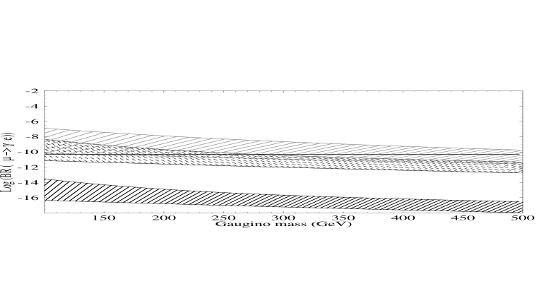
Figure 2: Predicted range for $BR(\mu\rightarrow e\gamma)$ as function of the gaugino mass in the three cases (see text): modular invariance (gray lines) , radiatively induced flavour violation with large Yukawa couplings (dashed lines) and small Yukawa couplings (black lines). The straight line correspond to the experimental bound on $BR(\mu\rightarrow e\gamma)<4.9~{}\cdot~{}10^{-11}$[19].

In order to determine the uncertainty of the theoretical predictions one has to vary the various supersymmetry breaking parameters in a range consistent with present experimental limits. For gaugino masses and the average scalar mass our choice is $m_{b}=100\ldots 500$ GeV, $m_{w}=100\ldots 500$ GeV, $M=100\ldots 500$ GeV, $A=0\ldots M$, $A+\mu\tan{\beta}=0\ldots M$. We know the transition amplitude only up to a factor ${\cal O}(1)$. We therefore also neglect neutralino and chargino mixings and we assumed for simplicity that the gauginos masses are equal. To estimate these uncertainties we increase the upper bound on the branching ratio by a factor of 5 and decrease the lower bound by a factor $1/5$. The result for $BR(\mu\rightarrow e\gamma)$ is shown in fig. 2 as function of the gaugino mass. The upper bound is given by the bino contribution with large mixing between ‘left’ and ‘right’ scalars ($M=100$ GeV, $A=M$, $A+\mu\tan{\beta}=M$); the lower limit is determined by the chargino contribution ($M=500$ GeV, $A=0$, $A+\mu\tan{\beta}=0$). For $\tau\rightarrow\mu\gamma$ the predicted branching ratio lies below the present upper experimental bound in all cases (cf. fig. (3)).

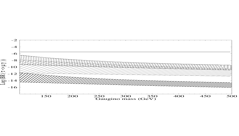
Figure 3: Predicted range for $BR(\tau\rightarrow\mu\gamma)$ as function of the gaugino mass in the three cases (see text): modular invariance (gray lines) , radiatively induced flavour violation with large Yukawa couplings (dashed lines) and small Yukawa couplings (black lines). The straight line correspond to the experimental bound on $BR(\tau\rightarrow\mu\gamma)<3~{}\cdot~{}10^{-6}$[19].

For most of the parameter space the prediction for $BR(\mu\rightarrow e\gamma)$ in models with modular invariance exceeds the experimental upper limit. Hence, this pattern of supersymmetry breaking appears to be disfavoured. For radiatively induced flavour violation and large Yukawa couplings the predicted range of branching ratios includes the present upper limit. An improvement of the sensitivity by two orders of magnitude would cover the entire parameter space. In the case of small Yukawa couplings the branching ratio is suppressed by $\epsilon^{4}\sim 10^{-5}$, and therefore far below the experimental limit.

For $\tau\rightarrow\mu\gamma$ the largest branching ratio is obtained for radiatively induced flavour mixing with large Yukawa couplings. This is a direct consequence of the large mixing between neutrinos of the second and the third generation. The observation of this radiative transition would therefore be of great significance.

References

[1]
Super-Kamiokande Collaboration, Y. Fukuda et al., Phys. Rev. Lett. 81 (1998) 62
[2]
T. Yanagida, in Workshop on unified Theories, KEK report
79-18 (1979) p. 95;
M. Gell-Mann, P. Ramond, R. Slansky, in Supergravity
(North Holland, Amsterdam, 1979)
eds. P. van Nieuwenhuizen and D. Freedman, p.315
[3]
C. D. Frogatt, H. B. Nielsen, Nucl. Phys. B 147 (1979) 277
[4]
J. Sato, T. Yanagida, Talk at Neutrino’98, hep-ph/9809307
[5]
P. Ramond, Talk at Neutrino’98, hep-ph/9809401
[6]
J. Bijnens, C. Wetterich, Nucl. Phys. B 292 (1987) 443
[7]
W. Buchmüller, T. Yanagida, Phys. Lett. B 445 (1999) 399
[8]
F. Vissani, JHEP11 (1998) 025
[9]
N. Irges, S. Lavignac, P. Ramond, Phys. Rev. D 58 (1998) 035003
[10]
For a review, see
H. P. Nilles, Phys. Rep. 110C (1984) 1
[11]
J. Ellis, D. V. Nanopoulos, Phys. Lett. B 110 (1982) 44
[12]
R. Barbieri, L. Hall, Phys. Lett. B 338 (1994) 212;
R. Barbieri, L. Hall, A. Strumia, Nucl. Phys. B 445 (1995) 219
[13]
J. Hisano, D. Nomura, T. Yanagida, Phys. Lett. B 437 (1998) 351;
J. Hisano, D. Nomura, hep-ph/9810479
[14]
G. K. Leontaris, N. D. Tracas, Phys. Lett. B 419 (1998) 206;
M. E. Gómez, G. K. Leontaris, S. Lola, J. D. Vergados, hep-ph/9810291
[15]
L. Ibáñez, D. Lüst, Nucl. Phys. B 382 (1992) 305
[16]
For a recent discussion and references, see
S. Lola, G. G. Ross, hep-ph/9902283
[17]
A. Brignole, L. E. Ibáñez, C. Muñoz, Nucl. Phys. B 422 (1994) 235
[18]
E. Dudas, S. Pokorski, C. A. Savoy, Phys. Lett. B 369 (1996) 255
[19]
C. Caso et al., Review of Particle Physics, Eur. Phys. J. C3, 1 (1998)