Are the Dirac particles of the Standard Model dynamically confined states in a higher-dimensional flat space?

Abstract

Some time ago Rubakov and Shaposhnikov suggested that elementary particles might be excitations trapped on a soliton in a flat higher dimensional space. They gave as an example $\phi^{4}$ theory in five dimensions with a bosonic excitation on a domain wall $\phi_{cl}$ in the fifth dimension. They also trapped a chiral Dirac particle on the domain wall with the interaction lagrangian $g\overline{\mathbf{\psi}}\mathbf{\phi\psi}$. The field equation for the Dirac field was $-i\sum_{\mathbf{\mu}=0}^{4}\mathbf{\gamma}^{\mathbf{\mu}}\partial_{\mathbf{\mu}}\mathbf{\psi}-g\mathbf{\phi\psi}=0.$ We show that a Dirac equation in eight flat dimensions with $-g\mathbf{\phi}$ replaced by a harmonic-oscillator “potential” in the four higher dimensions (plus a large constant $M_{0})$ generates bound states in approximate $SU\left(4\right)\times SU\left(2\right)$ representations. These representations have corresponding “orbital” times “spin” quantum numbers and bear some resemblance to the quarks and leptons of the Standard Model. Soliton-theory suggests that the harmonic-oscillator potential should rise only a finite amount. This will then limit the number of generations in a natural way. It will also mean that particles with sufficient energy might escape the well altogether and propagate freely in the higher dimensions. It may be worthwhile to search for a soliton (instanton?) which can confine Dirac particles in the manner of the harmonic-oscillator potential.

1 Introduction

Domain walls and other solitons play a central role in many theories of elementary particles. In 1983 Rubakov and Shaposhnikov (RS) suggested that solitons might even constitute an alternative to compactification in Kaluza-Klein and string models [1]. They gave as an example $\mathbf{\ \phi}^{4}$-theory in five flat (non-compact) dimensions, choosing

$$\mathcal{L}=\tfrac{1}{2}\sum_{\mu=0}^{4}\left(\frac{\partial\mathbf{\phi}}{\partial\mathbf{x}^{\mathbf{\mu}}}\right)\left(\frac{\partial\mathbf{\phi}}{\partial\mathbf{x}_{\mathbf{\mu}}}\right)+\tfrac{1}{2}m^{2}\mathbf{\phi}^{2}-\tfrac{1}{4}\lambda\mathbf{\phi}^{4},$$ (1)

with $\mathbf{\phi}$ a real, one-component field and $\mathbf{g}^{\mathbf{\mu\nu}}=$ diag$.\left(+,-,-,-;-\right).$ If $m^{2}>0,$ then domain-wall solutions can occur. RS noted that if a domain-wall appears and is assigned to the fifth dimension, then an excitation of the wall can be interpreted as a boson free to propagate in the four dimensions of ordinary space-time but trapped on the wall in the extra dimension. What sets this manner of confinement apart from ordinary compactification scenarios, of course, is that a particle of sufficient energy might escape confinement and propagate freely in all five dimensions.

RS also generated a massless (chiral) Dirac particle by adding to lagrangian 1 the terms

$$\mathcal{L}_{D}=i\overline{\mathbf{\psi}}\sum_{\mu=0}^{4}\mathbf{\gamma}^{\mathbf{\mu}}\partial_{\mathbf{\mu}}\mathbf{\psi}+g\overline{\mathbf{\psi}}\mathbf{\phi\psi,}$$ (2)

where $\ \mathbf{\gamma}^{\mathbf{\mu}}\mathbf{\gamma}^{\mathbf{\nu}}\mathbf{+\;\mathbf{\gamma}^{\mathbf{\nu}}\mathbf{\gamma}^{\mathbf{\mu}}=2g}^{\mathbf{\mu\nu}},\;\mathbf{\mu,\nu}=0,1,\,.\,.\,4.$  As in the case of the boson, the Dirac particle is free to propagate in $M^{4}$ but skates on the wall in the fifth flat dimension.

Trapping a Dirac particle on an extra flat dimension also plays a role in lattice gauge theories these days. To avoid Dirac-particle doubling, Kaplan introduced a fifth flat dimension and generated a massless Dirac particle with a lagrangian similar to that of Rubakov and Shaposhnikov [2]. When Kaplan’s lagrangian is expressed on a lattice, the second Weyl fermion appears on an opposite wall in the fifth dimension with exponentially vanishing overlap with the first Weyl fermion, thus getting around the no-go theorems [3]. Jansen provides a review of work following Kaplan’s original paper [4].

A question that naturally comes to mind is whether there exists a soliton in a larger space which can generate all three generations of quarks and leptons. RS remarked that if a domain wall could dynamically confine a particle in one flat extra dimension, then perhaps a vortex could confine it in two, a monopole in three, and an instanton in four flat extra dimensions. Could the mass-spectrum of such a confined particle exhibit the quantum numbers of the quarks and leptons?

For our part, we had carried out a study of the Klein-Gordon equation extended to eight flat dimensions $M^{4}\times\widetilde{R}^{4}$ and found that if we included a symmetrical harmonic-oscillator term in the four extra dimensions, then we obtained confined $SU\left(4\right)$ solutions suggestive of the three generations of quarks and leptons [5]. However a physical basis for the harmonic-oscillator term was lacking. Could a soliton (instanton?) provide the confinement?

In the remainder of this paper, we propose a Dirac field equation in eight flat dimensions which generates Dirac particles with quantum numbers suggestive of quarks and leptons. We will indicate how these particles might be coupled to gluons and the electroweak bosons in a manner consistent with a left-right symmetric extension of the Standard Model [7].

2 Domain walls in five dimensions

To motivate the extension to eight dimensions, let us review the $\mathbf{\phi}^{4}$-model in five dimensions. Lagrangian 1 generates the field equation

$$\sum_{\mathbf{\mu}=0}^{4}\partial^{\mathbf{\mu}}\partial_{\mathbf{\mu}}\mathbf{\phi}-m^{2}\mathbf{\phi}+\lambda\mathbf{\phi}^{3}=0$$ (3)

which admits the “kink” solution

$$\mathbf{\phi=}\left(m/\sqrt{\lambda}\right)\tanh\left[m\left(\widetilde{x}-\widetilde{x}_{0}\right)/\sqrt{2}\right]\equiv\widetilde{\phi}_{cl}.$$ (4)

(Here we denote the fifth dimension $x^{4}\equiv\widetilde{x},$ and set $\widetilde{x}_{0}$ equal to zero.) $\widetilde{\phi}_{cl}$ minimizes the action locally, and if $\mathbf{\phi}$ is expanded about it, then$\;\mathbf{\eta\equiv\phi-}\widetilde{\phi}_{cl}$ satisfies

$$\left(\sum_{\mathbf{\mu}=0}^{4}\partial^{\mathbf{\mu}}\partial_{\mathbf{\mu}}-m^{2}+3\lambda\widetilde{\phi}_{cl}^{2}\right)\mathbf{\eta}=0;$$ (5)

terms cubic and quartic in $\mathbf{\eta}$ are to be treated by standard perturbation theory. If we set $\mathbf{\eta=}\eta\left(x^{\mu}\right)\widetilde{\eta}\left(\widetilde{x}\right),$ then

$$\left(\square+M^{2}\right)\eta=0$$ (6)

where $\square$ is the d’Alembertian in $M^{4}$, and

$$\left(-\partial^{2}/\partial\widetilde{x}^{2}+3\lambda\widetilde{\phi}_{cl}^{2}-m^{2}\right)\widetilde{\eta}=M^{2}\widetilde{\eta}.$$ (7)

$M$ is taken to be the scalar boson’s mass. Eq. 7 is a one-dimensional Schrödinger-like equation that admits a massless solution (which merely corresponds to a translation of the soliton), a solution $\widetilde{\eta}_{3/2}=\sinh\widetilde{z}/\cosh^{2}\widetilde{z}$, ($\tilde{z}\equiv m\tilde{x}/\sqrt{2}$) with $M^{2}=\frac{3}{2}m^{2}$ which represents a boson trapped in the well, and continuum solutions $\widetilde{\eta}_{c}$ for $M^{2}\geq 2m^{2}$ which represent bosons free to propagate in all five dimensions [1, 8]. We have plotted $\widetilde{\eta}_{3/2}$ in Fig. 1 along with the confining potential $3\lambda\widetilde{\phi}_{cl}^{2}-m^{2}\equiv\tilde{V}$.

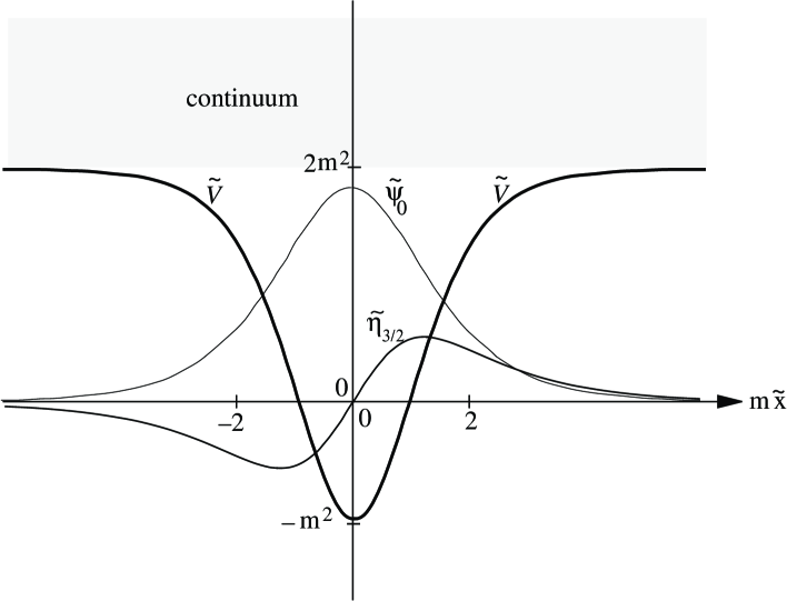
Figure 1: Confining potential $\widetilde{V}$ as a function of the extra dimension $\widetilde{x}$; 
$\widetilde{V}$ is generated by domain-wall solution $\widetilde{\phi}_{cl}$. Also shown is the wavefunction $\widetilde{\eta}_{3/2}$ of the boson trapped in the well, and the wavefunction $\widetilde{\psi}_{0}$ of a massless Dirac particle trapped on the wall, for $g=\sqrt{\lambda}.$

If lagrangian 1 is augmented by lagrangian 2, then minimizing the action yields the field equation

$$-i\sum_{\mathbf{\mu}=0}^{4}\mathbf{\gamma}^{\mathbf{\mu}}\partial_{\mathbf{\mu}}\mathbf{\psi}-g\mathbf{\phi\psi}=0.$$ (8)

If $\mathbf{\phi}$ is approximated by the domain-wall solution $\widetilde{\phi}_{cl}$, then

$$-i\sum_{\mathbf{\mu}=0}^{4}\mathbf{\gamma}^{\mathbf{\mu}}\partial_{\mathbf{\mu}}\mathbf{\psi}-g\widetilde{\phi}_{cl}\mathbf{\psi}=0.$$ (9)

This equation admits a solution $\mathbf{\psi=}\psi_{0,L}\widetilde{\psi}_{0}$, where $\psi_{0,L}$ is a left-helical, massless wavefunction in $M^{4}$ and

$$\widetilde{\psi}_{0}=\left(\cosh m\widetilde{x}/\sqrt{2}\right)^{-g\sqrt{2/\lambda}}.$$ (10)

$\widetilde{\psi}_{0}$ is plotted in Fig 1 for the case $g=\sqrt{\lambda}.$ (There is no massless right-helical solution.) There are also unconfined Dirac states of mass $\geq$ $gm/\sqrt{\lambda}.$

3 Eight-dimensional Dirac equation

Let us suppose that there exists a generalization of Eq. 9 in a higher-dimensional flat space of sufficient dimensionality to accommodate all of the quarks and leptons in the Standard Model. If so, then how many extra dimensions are required, and what kind of “potential” is needed? The difficulty is that $\widetilde{N}$-dimensional extensions naturally lead to $SO(\widetilde{N})$-symmetry groups, whereas quarks require $SU(\widetilde{N})$-type symmetry. However, if the potential generates harmonic-oscillator states, then these states will be representations of an $SU(\widetilde{N})$-algebra. (See Appendix A.). Since quarks exhibit $SU(3)$ color-symmetry, this would be a vote for $\widetilde{N}=3$ and a symmetrical harmonic-oscillator potential. Because the coordinates are real, only the (triangular) 1, 3, 6, 10, . . .   representations would appear, each just once [5]. The 3 might correspond to a quark. (The 1 might correspond to a “lepton”. The 6, 10, . . would be new species of Dirac particles.) The spin-degree of freedom might simulate weak isospin.

To accommodate all three generations of quarks and leptons, a higher symmetry would be required. $SU\left(4\right)$ might suffice. For four (real) extra coordinates, the $SU\left(4\right)$-wavefunctions have the tetrahedral 1, 4, 10, 20, . . representations, with the 4 breaking to 1$+$3, the 10 breaking to 1$+$3$+$6, etc. The $SU\left(4\right)$-1 might represent a first-generation “lepton”, the 1$+$3 = 4 a second-generation “lepton” and a first-generation “quark”, etc. Weight diagrams of the lowest $SU\left(4\right)$-multiplets are sketched in Fig. 2.

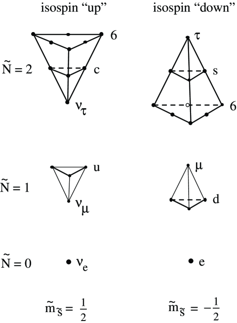
Figure 2: Weight diagrams of lowest lying $SU\left(4\right)\times SU\left(2\right)$ multiplets of Eqs. 20 and 24. Diagrams plotted vs. principal $SU\left(4\right)$ quantum number $\widetilde{N}$ and $SU\left(2\right)$ quantum number $\tilde{m}_{\tilde{s}}$ . “Quarks” and “leptons” suggested by these quantum numbers are indicated. All members of a given multiplet are degenerate in mass. However the weight diagrams are oriented so that heavier particles appear above lighter particles; i.e., the $\widetilde{n}_{4}$ (“generation-number”) axis points downward for $\tilde{m}_{\tilde{s}}=\frac{1}{2}$ multiplets and upward for $\tilde{m}_{\tilde{s}}=-\frac{1}{2}$ multiplets.

Could a harmonic-oscillator “potential” actually exist in a higher dimensional flat space? Possibly. Dvali and Shifman have shown that for some topological defects, in supersymmetric theories at least, such oscillator-type potentials appear naturally [9].

However a Dirac equation with a harmonic-oscillator potential will not necessarily generate harmonic-oscillator wavefunctions. A Schrödinger equation or a Klein-Gordon equation will [5], but a Dirac equation might not because the Dirac operator “squares” the potential. However consider the hydrogen atom in ordinary space-time. We know that the Coulomb potential in the Dirac equation of the H-atom reappears as the Coulomb potential in the (Pauli-reduced) Schrödinger equation. This happens because the rest-mass of the electron is very large compared to the kinetic and potential energies of the electron and thereby minimizes the symmetry-breaking “small” components. Similarly if we extend Eq. 8 to eight flat dimensions, replace the domain wall with a symmetrical harmonic-oscillator potential $\mathbf{V}$ in the four extra dimensions and insert a large “rest-mass” $M_{0}$, yielding

$$\left(-i\sum_{\mathbf{\mu}=0}^{7}\mathbf{\gamma}^{\mathbf{\mu}}\partial_{\mathbf{\mu}}\;\mathbf{+\;V}+M_{0}\right)\mathbf{\psi}=0,$$ (11)

then $\mathbf{V}$ reappears unsquared in the two-component reduction of the Dirac equation in the four higher dimensions. This Pauli equation will generate exact $SU\left(4\right)$ harmonic-oscillator “large” components, and the symmetry-breaking lower components will be small. We will show this directly.

Let $\mathbf{\gamma}^{\mathbf{\mu}}\mathbf{\gamma}^{\mathbf{\nu}}+\mathbf{\gamma}^{\mathbf{\nu}}\mathbf{\gamma}^{\mathbf{\mu}}=2\mathbf{g}^{\mathbf{\mu\nu}},$ $\mathbf{\mu,\nu}=0,$ $1,$ $\;7,$ where the metric-tensor $\mathbf{g}^{\mathbf{\mu\nu}}$ = diag.$\left(+,-,-,\ldots,-\right).$ A convenient representation of the gamma-matrices is the “chiral” set

$$\mathbf{\gamma}^{\mathbf{\mu}}=\left\{\begin{array}[]{ll}\gamma^{\mu}\otimes\widetilde{\gamma}^{5},&\mathbf{\mu}=\mu=0,1,2,3,\\ 1\otimes\widetilde{\gamma}^{5}\widetilde{\gamma}^{\widetilde{\mu}},&\mathbf{\mu}=\widetilde{\mu}+3=4,5,6,7\end{array}\right.$$ (12)

where $\gamma^{\mu},$ $\;\mu=0,\;1,\;2,\;3$ is any standard set of Dirac matrices while

$\widetilde{\gamma}^{\widetilde{j}}=\left(\begin{array}[]{ll}\;\;0&i\widetilde{\sigma}^{\widetilde{j}}\\ -i\widetilde{\sigma}^{\widetilde{j}}&0\end{array}\right),\;\widetilde{j}=1,2,3,$ $\;\;\;\widetilde{\gamma}^{4}=\left(\begin{array}[]{ll}0&1\\ 1&0\end{array}\right),$   and $\qquad\widetilde{\gamma}^{5}=\left(\begin{array}[]{ll}1&\;\,0\\ 0&-1\end{array}\right).$ The $\widetilde{\sigma}^{\widetilde{j}}$ are the $2\times 2$ Pauli spin matrices. The potential $\mathbf{V}=1\otimes\tilde{\gamma}^{5}\tilde{V}\left(\tilde{x}\right)$, where $\tilde{V}\$has the harmonic-oscillator form.

If one multiplies Eq. 11 by $1\otimes\widetilde{\gamma}^{5}$ and sets $\mathbf{\psi}=\psi\left(x\right)\otimes\widetilde{\psi}\left(\tilde{x}\right)$ , then (11) separates into

$$\left(-i\mathbf{\hbox to0.0pt{/\hss}\nabla}+M\right)\psi\left(x\right)=0$$ (13)

and

$$\left(-i\tilde{\hbox to0.0pt{/\hss}\nabla}+\widetilde{V}+\widetilde{\gamma}^{5}M_{0}\right)\widetilde{\psi}=M\widetilde{\psi,}$$ (14)

where $\mathbf{\hbox to0.0pt{/\hss}\nabla}=\sum_{\mu=0}^{3}\gamma^{\mu}\partial/\partial x^{\mu}$ and $\tilde{\hbox to0.0pt{/\hss}\nabla}=\sum_{\widetilde{\mu}=1}^{4}\widetilde{\gamma}^{\widetilde{\mu}}\partial/\partial\widetilde{x}^{\widetilde{\mu}}$. We have denoted $\left(\mathbf{x}^{4},\mathbf{x}^{5},\mathbf{x}^{6},\mathbf{x}^{7}\right)\equiv\left(\widetilde{x}^{1},\widetilde{x}^{2},\widetilde{x}^{3},\widetilde{x}^{4}\right).$ $M$ (not $M_{0})$ is taken to be the rest-mass of the Dirac particle in ordinary space-time. In practice, one solves Eq. 14 for the eigenfunction $\widetilde{\psi}$ and eigenmass $M$, then inserts $M$ in Dirac Eq. 13.

The Dirac equation in the extra dimensions may be expanded to

$$\left(\begin{array}[]{ll}\widetilde{V}+M_{0}-M&\qquad\widetilde{D}\\ \qquad\widetilde{D}^{\dagger}&\widetilde{V}-M_{0}-M\end{array}\right)\left(\begin{array}[]{l}\widetilde{\phi}\\ \widetilde{\chi}\end{array}\right)\;=\;0,$$ (15)

where

$$\widetilde{D}\;=\;\left(\begin{array}[]{ll}\widetilde{\partial}_{3}-i\widetilde{\partial}_{4},&\quad\widetilde{\partial}_{1}-i\widetilde{\partial}_{2}\\ \widetilde{\partial}_{1}+i\widetilde{\partial}_{2},&-\;\widetilde{\partial}_{3}-i\widetilde{\partial}_{4}\end{array}\right)$$ (16)

with $\widetilde{\partial}_{\widetilde{\mu}}\equiv\partial/\partial\widetilde{x}^{\widetilde{\mu}},\;\widetilde{\mu}=1,\;2,\;3,\;4.$  If $M_{0}\gg\left\langle\widetilde{V}\right\rangle$ and $M\sim M_{0},$ then

$$\widetilde{\chi}\thickapprox\frac{1}{2M_{0}}\widetilde{D}^{\dagger}\widetilde{\phi},$$ (17)

yielding

$$\left(\widetilde{V}+M_{0}-M\right)\widetilde{\phi}\,+\,\widetilde{D}\left(2M_{0}\right)^{-1}\widetilde{D}^{\dagger}\widetilde{\phi}=0.$$ (18)

$\widetilde{D}\widetilde{D}^{\dagger}=\widetilde{D}^{\dagger}\widetilde{D}=-\;\tilde{\square}\cdot\widetilde{1}_{2\times 2}$ where $\tilde{\square}$ is the four-dimensional laplacian in $\widetilde{R}^{4},$ so Eq.18 reduces to

$$\left(-\;\frac{1}{2M_{0}}\tilde{\square}+\widetilde{V}\right)\widetilde{\phi}=\left(M-M_{0}\right)\widetilde{\phi}.$$ (19)

Eq. 19 is analogous to the Pauli reduction of the time-independent Dirac equation in ordinary space, with $M-M_{0}$ playing the role of the kinetic energy. If $\widetilde{V}$ is a symmetrical harmonic-oscillator potential, then solutions $\tilde{\phi}$ comprise an exact representation of an $SU\left(4\right)$-algebra. In particular, if $\widetilde{V}$=$\widetilde{\alpha}^{3}\widetilde{X}^{2},$ where $\widetilde{\alpha}$ is an adjustable real constant and $\widetilde{X}^{2}=\sum_{\widetilde{\mu}=1}^{4}\left(\widetilde{x}^{\widetilde{\mu}}\right)^{2},$ then

$$\tilde{\phi}\,=\,\prod_{\tilde{\mu}=1}^{4}\tilde{\phi}_{\tilde{n}_{\tilde{\mu}}}\left(\tilde{\beta}\tilde{x}^{\tilde{\mu}}\right)\,\equiv\,\tilde{\phi}_{\tilde{n}_{1}\tilde{n}_{2}\tilde{n}_{3}\tilde{n}_{4}}\,\equiv\,\tilde{\phi}_{\tilde{n}},$$ (20)

a product of (unnormalized) harmonic-oscillator functions

$$\tilde{\phi}_{\tilde{n}_{\tilde{\mu}}}\left(\tilde{\beta}\tilde{x}^{\tilde{\mu}}\right)=H_{\tilde{n}_{\tilde{\mu}}}\left(\tilde{\beta}\tilde{x}^{\tilde{\mu}}\right)\exp\left[-\tfrac{1}{2}\tilde{\beta}^{2}(\tilde{x}^{\tilde{\mu}})^{2}\right],\;\;\;\;\tilde{\mu}=1,\;\,2,\;3,\;4;$$ (21)

here $\tilde{\beta}^{4}=2M_{0}\tilde{\alpha}^{3}$ and $H_{\tilde{n}_{\tilde{\mu}}}$ is a Hermite polynomial of degree $\tilde{n}_{\tilde{\mu}}=0,\;1,\;2,\;3,\;.\;.$ The associated eigenmass $M=M_{0}+\left(2\tilde{N}+4\right)(\tilde{\beta}^{2}/2M_{0})\equiv\overline{M}^{\left(\tilde{N}\right)},$ where

$$\tilde{N}=\tilde{n}_{1}+\tilde{n}_{2}+\tilde{n}_{3}+\tilde{n}_{4}=0,\;1,\;2,\;3,\;.\;.$$ (22)

(See Appendix A.)

Actually the solutions to Pauli equation 19 exhibit a higher symmetry than $SU\left(4\right)$ since they also include constant two-component spinors $\tilde{\xi}_{\tilde{m}_{\tilde{s}}}={\binom{1}{0}}$ and ${\binom{0}{1}}$ which are representations of $SU\left(2\right)$.  Thus

$$\tilde{\phi}\,=\,\tilde{\phi}_{\tilde{n}_{1}\tilde{n}_{2}\tilde{n}_{3}\tilde{n}_{4}}\tilde{\xi}_{\tilde{m}_{\tilde{s}}}\,\equiv\,\tilde{\phi}_{\tilde{n},\tilde{m}_{\tilde{s}}},$$ (23)

where the $\tilde{\phi}_{\tilde{n},\tilde{m}_{\tilde{s}}}$ are representations of $SU\left(4\right)\times SU\left(2\right).$

The solutions to the Dirac equation in the extra dimensions, Eq. 14, are thus

$$\tilde{\psi}=\left(\begin{array}[]{l}\tilde{\phi}\\ \tilde{\chi}\end{array}\right)\approx\left(\begin{array}[]{l}\;\;\;\;\;\;\tilde{\phi}_{\tilde{n},\tilde{m}_{\tilde{s}}}\\ \frac{1}{2M_{0}}\tilde{D}^{\dagger}\tilde{\phi}_{\tilde{n},\tilde{m}_{\tilde{s}}}\end{array}\right)\equiv\tilde{\psi}_{\tilde{n}_{1}\tilde{n}_{2}\tilde{n}_{3}\tilde{n}_{4}\tilde{m}_{\tilde{s}}}\equiv\tilde{\psi}_{\tilde{n},\tilde{m}_{\tilde{s}}},$$ (24)

with the same eigenmasses $\overline{M}^{\left(\tilde{N}\right)}.$  Since $\tilde{\chi}\thickapprox\frac{1}{2M_{0}}\tilde{D}^{\dagger}\tilde{\phi}_{\tilde{n},\tilde{m}_{\tilde{s}}}\backsim\frac{1}{2M_{0}}\tilde{\beta}\tilde{\phi}=\left(\frac{\tilde{\alpha}}{2M_{0}}\right)^{3/4}\tilde{\phi}$, these lower components vanish in the limit as $\tilde{\alpha}/2M_{0}\rightarrow 0$ . In this limit, solutions $\tilde{\psi}$ will have the same symmetry as the $\tilde{\phi},$ namely $SU\left(4\right)\times SU\left(2\right).$

How do the $\tilde{\psi}_{\tilde{n},\tilde{m}_{\tilde{s}}}$ suggest quarks and leptons? Consider the eigenfunctions of the $SU\left(4\right)\;$4 with, say, $SU\left(2\right)$ spin “up”. The 4’s upper components $\tilde{\phi}$ are $\tilde{x}^{1}\tilde{F}{\binom{1}{0}},\;\tilde{x}^{2}\tilde{F}{\binom{1}{0}},\;\tilde{x}^{3}\tilde{F}{\binom{1}{0}},$ and $\tilde{x}^{4}\tilde{F}{\binom{1}{0}},$ where $\tilde{F}\equiv\exp(-\frac{1}{2}\tilde{\beta}^{2}\tilde{X}^{2}).$ The triplet-subset $\left(\tilde{x}^{1},\;\tilde{x}^{2},\;\tilde{x}^{3}\right)\tilde{F}{\binom{1}{0}}$ , say, is an $SU\left(3\right)$ 3 and can be coupled to another 3 and an $SU\left(3\right)$ 8 (gluon) to yield an invariant scalar, as we show in Sec. IV. Thus the 3 resembles a color triplet. In addition, the 3 with spin ${\binom{1}{0}}$ and the 3 from the other 4 with spin ${\binom{0}{1}}$ constitute an $SU\left(2\right)$ 2 and can be coupled to an isospin-3 intermediate vector-boson to yield another invariant scalar. Thus the 2 suggests a weak-isospin doublet. In this way the $SU\left(3\right)\times SU\left(2\right)$ $\left(\mathbf{3},\mathbf{2}\right)$ resembles a quark.

The remaining wavefunction of the 4, $\tilde{x}^{4}\tilde{F}{\binom{1}{0}}$, will be an $SU\left(4\right)$ “color”-singlet, but still a member of an $SU\left(2\right)$-doublet. Thus it can be coupled to an EW-boson, and suggests a lepton.

As noted earlier, weight diagrams of these multiplets are sketched in Fig. 2, for $\tilde{N}=0,\;1,$ and $2$. Dirac particles suggested by these multiplets are indicated.

Dirac equation 11 predicts only two bound spin states for each “orbital” wavefunction $\tilde{\phi}_{\tilde{n}_{1}\tilde{n}_{2}\tilde{n}_{3}\tilde{n}_{4}}$, even though the Dirac wavefunction has four components. This is analogous to the Dirac equation of the hydrogen atom which predicts just two bound spin states for each orbital wavefunction rather than four; the other two spin states correspond to positron-proton states and of course are not bound. If the H-atom’s confining potential were a scalar $\left(-e^{2}/r\right)$ rather than the fourth component of a vector $\left(-\gamma^{0}e^{2}/r\right)$, then the positron-proton states would also be bound, at a negative energy $E\thicksim-m$.

Similarly if the potential V in eight-dimensional equation 11 were $\tilde{V}$ rather than $\tilde{\gamma}^{5}\tilde{V},$ then a second spectrum of confined states would appear with large lower components $\tilde{\chi}\,\thickapprox\,\tilde{\phi}_{\tilde{n}_{1}\tilde{n}_{2}\tilde{n}_{3}\tilde{n}_{4}}\tilde{\xi}_{\tilde{m}_{\tilde{s}}}$ , small upper components $\tilde{\phi},$ and masses $M=-\overline{M}^{\left(\tilde{N}\right)}$. The masses of this spectrum would be identical to those of the positive spectrum since a negative mass can be interpreted as a positive mass with the ordinary space-time spinor $\psi$ replaced by $\gamma^{5}\psi$. This would yield twice too many “weak-isospin” states. Thus the $\tilde{\gamma}^{5}\tilde{V}$ structure is indicated.

The potential $\tilde{V}$ generated by a soliton in five-dimensional $\mathbf{\phi}^{4}$-theory does not rise to infinity like a pure HO potential, of course. Instead it reaches an upper limit, as shown in Fig. 1. Similarly, any potential generated by a soliton in a higher dimensional space might be expected to rise no higher than some maximum value, call it $\tilde{V}_{\infty}$. In the case of Dirac equation 11, if this maximum height $\tilde{V}_{\infty}$ is $<<M_{0},$ then it is easy to show that the equation generates confined states with masses $M$ in the range $M_{0}<M<M_{0}+V_{\infty}$ and free states (able to propagate anywhere in $M^{4}\times\tilde{R}^{4}$) with masses $M$ in the range $M_{0}+\tilde{V}_{\infty}<M<\infty$. Because Eq. 11 is a relativistic equation, it also admits free solutions with negative masses in the range $-\infty<M<-M_{0}+\tilde{V}_{\infty}$. Again, if the ordinary space-time spinor $\psi$ is replaced by $\gamma^{5}\psi,$ then the masses in this third spectrum change sign and span the range $M_{0}-\tilde{V}_{\infty}<M<\infty$.

Now this third mass-spectrum of free particles completely overlaps the discrete spectrum of trapped particles, so is immediately ruled out by experiment. However if all three spectra are lowered by an amount, say, $M_{0},$ so that $M$ is restricted to the three intervals $0<M<\tilde{V}_{\infty}$, $\tilde{V}_{\infty}<M<\infty,$ and $-\infty<M<-2M_{0}+\tilde{V}_{\infty},\;\;$then the third spectrum is equivalent to $2M_{0}-\tilde{V}_{\infty}<M<$ $\infty$ and neither it nor the other continuous spectrum overlaps the discrete spectrum.  Furthermore this lowers the threshold of discrete particles from $M_{0},$ which is far too massive, to $0,$ closer to experiment.

Lowering these spectra can be accomplished, admittedly ad hoc, simply by subtracting $M_{0}$ from $\tilde{V}$. Thus we will set

$$\mathbf{V}=1\otimes\tilde{\gamma}^{5}\left(\tilde{V}-M_{0}\right),$$ (25)

where $\tilde{V}$ is a HO-like potential that rises only to $\tilde{V}_{\infty}$, analogous to the $\tilde{V}$ in Fig. 1. If lim${}_{\tilde{X}\rightarrow 0}\tilde{V}=\tilde{\alpha}^{3}\tilde{X}^{2}$ and $\left(2\tilde{N}+4\right)\tilde{\beta}^{2}/2M_{0}<<\tilde{V}_{\infty}$, then

$$M\thickapprox\left(2\tilde{N}+4\right)(\tilde{\beta}^{2}/2M_{0})=\left(2\tilde{N}+4\right)(\tilde{\alpha}^{3}/2M_{0})^{1/2}\equiv M^{\left(\tilde{N}\right)},$$ (26)

$\tilde{N}=0,\;1,\;2,\;.\;.\;.$

The possibility of continuous mass spectra raises an interesting question. If we really are trapped in a topological or non-topological defect in a higher-dimensional flat space, then are there particles freely ranging in this extended space that could invade our local territory? Could they sometimes appear even at energies above the Greisen-Zatsepin-Kus’min cutoff $[11]$ $(\thicksim 5\cdot 10^{19}$ eV)? And might we be able to propel Dirac particles from our local space into that continuum? The threshold for ejecting particles into the conjectured continuum may lie just above the capability of present-day machines. In that case, there might be events such as $e^{+}+e^{-}\rightarrow$ $2\;$free Dirac particles [1], appearing to be $e^{+}+e^{-}\rightarrow$ nothing.

An interesting question is also posed by the discrete spectrum. If quarks and leptons really do occur in $SU\left(4\right)$ multiplets, then $SU\left(3\right)$ 6s should accompany the charm and strange quarks in the $SU\left(4\right)$ 10s (see Fig. 2), and $SU\left(3\right)$ 6s and 10s should accompany the top and bottom quarks in $SU\left(4\right)$ 20s (not shown). Such particles have never been seen. If they do exist, then they apparently do not interact with either the electroweak bosons or gluons. This should make them good candidates for dark matter.

The discrete spectrum also suggests fourth-generation leptons, call them $\nu_{4}$ and $l_{4}.$ These particles would accompany the top and bottom quarks in $SU\left(4\right)$ 20s. Such particles have never been seen either. Present-day experimental limits [11] would place them above about $45$ GeV.

Of course, just as in nuclear physics, not every member of a multiplet need be bound. This might explain the absence of at least some of the 6s and 10s and leptons.

Another interesting question has to do with the size of the bound states in the extra dimensions. Their widths can be easily calculated if the confining “potential” is taken to be a harmonic oscillator. If we adopt as a measure of this width (squared)

$$\int\tilde{\psi}_{\widetilde{n}}^{\dagger}\tilde{X}^{2}\tilde{\psi}_{\widetilde{n}}d^{4}\tilde{x}\approx\int\tilde{\phi}_{\widetilde{n}}^{\dagger}\tilde{X}^{2}\tilde{\phi}_{\widetilde{n}}d^{4}\tilde{x}\equiv\tilde{X}_{rms}^{2}$$ (27)

[recall that $\widetilde{X}^{2}=\sum_{\widetilde{\mu}=1}^{4}\left(\widetilde{x}^{\widetilde{\mu}}\right)^{2}$], then one can readily show that $\tilde{X}_{rms}^{2}=\left(\tilde{N}+2\right)/\tilde{\beta}^{2}.$ Folding in Eq. 26 and restoring $\mathbf{\hbox to0.0pt{/\hss}}h$ and $c$ yield

$$\tilde{X}_{\widetilde{N}}=\left(\tilde{N}+2\right)\left(M^{\left(\widetilde{N}\right)}M_{0}\right)^{-\frac{1}{2}}\mathbf{\hbox to0.0pt{/\hss}}h/c\equiv\tilde{X}_{rms}.$$ (28)

As for numbers, if we choose $M_{0}=100\;$TeV and adjust $\tilde{\alpha}$ to fit an up-quark mass of $6$ MeV, then $\tilde{X}_{rms}=0.024$ F (with $\tilde{\alpha}=585$ MeV). If we set $M_{0}=10^{4}\;$TeV, then $\tilde{X}_{rms}=0.0024$ F (with $\tilde{\alpha}=2710$ MeV).

Now according to the Particle Data Group [11], leptons and quarks have radii no greater than the order of $10^{-4}$ F. However these are radii in ordinary space-time. They can be measured, e.g., by probing the Dirac particle with photon-wavefunctions $\exp\left(-ip\cdot x\right)$ over a range of momenta $\overrightarrow{p}$ and taking the Fourier transform. To measure the size of a Dirac particle in both ordinary space and extended space, one could figuratively probe the particle with “photon” wavefunctions $\exp\left(-ip\cdot x+i\tilde{p}\cdot\tilde{x}\right)$ where now the higher dimensional “momentum” $\tilde{p}$ would also range over some interval. However these would be the wavefunctions of probes free to propagate in all of the dimensions, higher and lower. Even if such particles were to exist, we would only have access to the photons confined in $M^{4}.$ These ordinary photons have just a single wavefunction in the higher dimensions (more kinds of wavefunctions would mean more kinds of photons), so they always weight the wavefunction of the Dirac particle the same way in the higher dimensions and tell us nothing about its higher-dimensional structure. If this is typical of all types of higher-dimensional reactions measurable by us, then the size of the Dirac particles in the extra dimensions is not subject to the Particle Data Group limits.

4 Interaction of Dirac particles with gauge fields

4.1 QCD interaction

In this section we will indicate how the “quark” solutions of Eq. 11 might be combined with a “gluon” gauge field to reproduce the QCD interaction lagrangian in the limit as $V_{\infty}\rightarrow\infty$. Consider the eight-dimensional interaction lagrangian

$$\mathcal{L}_{int}=\tfrac{1}{\sqrt{2}}g_{s}\sum_{\mu=0}^{3}\sum_{\tilde{i},\tilde{j}=1}^{3}\overline{\mathbf{\psi}}\gamma^{\mu}\tilde{E}_{\tilde{i}\tilde{j}}\mathbf{G}_{\mu}^{\tilde{i}\tilde{j}}\mathbf{\psi,}$$ (29)

where $\mathbf{G}_{\mu}^{\tilde{i}\tilde{j}}$ is the “gauge field” and the $\tilde{E}_{\tilde{i}\tilde{j}}$ are the $SU\left(3\right)$-generators defined by Eq. 47 in Appendix A. It may not be unreasonable to suppose that $\mathbf{G}_{\mu}^{\tilde{i}\tilde{j}}=G_{\mu}(x)\tilde{G}^{\tilde{i}\tilde{j}}(\tilde{x})$, in which case ordinary space-time quantities such as energy-momentum, angular momentum, etc. are conserved. In this case, $\mathcal{L}_{int}$ will be a sum over terms of the sort

$$\tfrac{1}{\sqrt{2}}g_{s}\overline{\psi}_{f}\left(x\right)\gamma^{\mu}G_{s,\mu}\left(x\right)\psi_{i}\left(x\right)\cdot\overline{\tilde{\psi}}_{\tilde{f}}(\tilde{x})\tilde{E}_{\tilde{i}\tilde{j}}\tilde{G}_{\tilde{s}}^{\tilde{i}\tilde{j}}(\tilde{x})\tilde{\psi}_{\tilde{i}}(\tilde{x}),$$ (30)

where Dirac and Bose states are identified by $f$, $i$, and $s$ in $M^{4}$ and $\tilde{f}$, $\tilde{i}$, and $\tilde{s}$ in $\tilde{R}^{4}$. ($\overline{\tilde{\psi}}=\tilde{\psi}^{\dagger}\tilde{\gamma}^{5}.)$ In the case of the bound-state solutions $\tilde{\psi}_{\widetilde{n}_{1}\widetilde{n}_{2}\widetilde{n}_{3}\widetilde{n}_{4}\widetilde{m}_{\tilde{s}}},$ the field $\tilde{G}_{\tilde{s}}^{\tilde{i}\tilde{j}}(\tilde{x})$ can cause transitions to different “families” ($\widetilde{n}_{4})$, to different $SU\left(3\right)$-multiplets $(\widetilde{N}^{\prime}=\widetilde{n}_{1}+\widetilde{n}_{2}+\widetilde{n}_{3})$ (e.g., quark$\rightarrow$ lepton), and to the opposite “weak-isospin” state ($\widetilde{m}_{\tilde{s}}$), all of which are inconsistent with QCD. However if $\tilde{G}_{\tilde{s}}^{\tilde{i}\tilde{j}}(\tilde{x})$ is essentially constant over the range of integration of $\overline{\tilde{\psi}}_{\tilde{f}}(\tilde{x})\tilde{E}_{\tilde{i}\tilde{j}}\tilde{G}_{\tilde{s}}^{\tilde{i}\tilde{j}}(\tilde{x})\tilde{\psi}_{\tilde{i}}(\tilde{x})$ in $\tilde{R}^{4}$, then none of these transitions can take place due to the orthogonality of the harmonic-oscillator functions, at least in the limit $\tilde{\alpha}/2M_{0}\rightarrow 0$ where $\tilde{\psi}\rightarrow\left(\tilde{\phi}_{\widetilde{n}_{1}\widetilde{n}_{2}\widetilde{n}_{3}\widetilde{n}_{4,}\widetilde{m}_{\tilde{s}}}(\tilde{x}),\;0\right)^{T}$. An example of a field that would be essentially constant over the range of integration is $\tilde{G}_{\tilde{s}}^{\tilde{i}\tilde{j}}(\tilde{x})=\widehat{G}_{\tilde{s}}^{\tilde{i}\tilde{j}}\exp\left(-\frac{1}{2}\tilde{\gamma}^{2}\tilde{X}^{2}\right)$, where the range $\tilde{\gamma}^{-1}$ of the gluon field is much greater than the range $\tilde{\beta}^{-1}$ of the Dirac-particle fields $\left(\tilde{\gamma}^{-1}>>\tilde{\beta}^{-1}\right)$; $\widehat{G}_{\tilde{s}}^{\tilde{i}\tilde{j}}$ is a constant which identifies the particular gluon field $\tilde{s}$.

Lagrangian 30 is still not consistent with QCD since $\tilde{\psi}$ can be any $SU\left(3\right)$-multiplet: 1, 3, 6, 10, . . . However if we limit the $SU\left(3\right)$-states to just 3s ($\widetilde{n}_{1}+\widetilde{n}_{2}+\widetilde{n}_{3}=1$ “quarks”) and 1s ($\widetilde{n}_{1}+\widetilde{n}_{2}+\widetilde{n}_{3}=0$ “leptons”), then the lagrangian is equivalent to the QCD lagrangian, as we will now show. One can integrate over $\tilde{R}^{4}$ and replace the $\tilde{\phi}_{\widetilde{n}_{1}\widetilde{n}_{2}\widetilde{n}_{3}\widetilde{n}_{4,}\widetilde{m}_{\tilde{s}}}(\tilde{x})$ by unit column vectors $\widehat{\phi}_{\widetilde{n}_{1}\widetilde{n}_{2}\widetilde{n}_{3}\widetilde{n}_{4,}\widetilde{m}_{\tilde{s}}}=\widehat{\phi}_{\widetilde{n}_{1}\widetilde{n}_{2}\widetilde{n}_{3}}\otimes\widehat{\phi}_{\widetilde{n}_{4}}\otimes\tilde{\xi}_{\tilde{m}_{\tilde{s}}}$, where the $\widehat{\phi}_{\widetilde{n}_{1}\widetilde{n}_{2}\widetilde{n}_{3}}\equiv\widehat{\phi}_{color}$ comprise the “color” states [ $\widehat{\phi}_{100}=(1,0,0)^{T},$ $\widehat{\phi}_{010}=(0,1,0)^{T},$ and $\widehat{\phi}_{001}=(0,0,1)^{T}$], $\widehat{\phi}_{\widetilde{n}_{4}}$ is a column vector with an element for each “generation”, and $\tilde{\xi}_{\tilde{m}_{\tilde{s}}}=(1,0)^{T}$ or $(0,1)^{T}$, the previously defined “weak-isospin” spinor. The operators $\tilde{E}_{\tilde{i}\tilde{j}}(\tilde{x},$ $\partial\tilde{x})$ can similarly be replaced by $3\times 3$ matrices $\widehat{E}_{\tilde{i}\tilde{j}},$ where

$$\widehat{E}_{11}=\left(\begin{array}[]{ccc}\frac{2}{3}&0&0\\ 0&-\frac{1}{3}&0\\ 0&0&-\frac{1}{3}\end{array}\right),\;\widehat{E}_{12}=\left(\begin{array}[]{lll}0&1&0\\ 0&0&0\\ 0&0&0\end{array}\right),\;\widehat{E}_{13}=\left(\begin{array}[]{lll}0&0&1\\ 0&0&0\\ 0&0&0\end{array}\right)$$ (31)

and similarly for $\widehat{E}_{2\tilde{j}}$ and $\widehat{E}_{3\tilde{j}},\;\tilde{j}=1,\;2,\;3$. The interaction lagrangian now takes the form

$$\widehat{\mathcal{L}}_{int}=\tfrac{1}{\sqrt{2}}g_{s}\sum_{\mu=0}^{3}\sum_{\tilde{i},\tilde{j}=1}^{3}\overline{\widehat{\mathbf{\psi}}}\gamma^{\mu}\widehat{E}_{\tilde{i}\tilde{j}}\widehat{\mathbf{G}}_{\mu}^{\tilde{i}\tilde{j}}\widehat{\mathbf{\psi}},$$ (32)

where $\widehat{\mathbf{\psi}}$ is a sum over states $\psi\left(x\right)\otimes\widehat{\phi}_{color}\otimes\widehat{\phi}_{\widetilde{n}_{4}}\otimes\tilde{\xi}_{\tilde{m}_{\tilde{s}}}$ and $\widehat{\mathbf{G}}_{\mu}^{\tilde{i}\tilde{j}}$ is a sum over states $G_{\mu}\left(x\right)\widehat{G}^{\tilde{i}\tilde{j}}$. This lagrangian equals the QCD lagrangian [11]

$$\mathcal{L}_{int}^{\scriptstyle QCD}=\tfrac{1}{2}g_{s}\sum_{\mu=0}^{3}\sum_{a=1}^{8}\overline{\widehat{\mathbf{\psi}}}\gamma^{\mu}\lambda^{a}\mathbf{G}_{\mu}^{a}\widehat{\mathbf{\psi}},$$ (33)

where the $\lambda^{a}$ are the Gell-Mann $3\times 3\;SU\left(3\right)$ matrices, if the QCD gauge fields

$$\mathbf{G}_{\mu}^{1}=\tfrac{1}{\sqrt{2}}\left(\widehat{\mathbf{G}}_{\mu}^{12}+\widehat{\mathbf{G}}_{\mu}^{21}\right),\ \;\mathbf{G}_{\mu}^{2}=\tfrac{i}{\sqrt{2}}\left(\widehat{\mathbf{G}}_{\mu}^{12}-\widehat{\mathbf{G}}_{\mu}^{21}\right),\;\;$$

$$\mathbf{G}_{\mu}^{3}=\tfrac{1}{\sqrt{2}}\left(\widehat{\mathbf{G}}_{\mu}^{11}-\widehat{\mathbf{G}}_{\mu}^{22}\right),\;\;\mathbf{G}_{\mu}^{4}=\tfrac{1}{\sqrt{2}}\left(\widehat{\mathbf{G}}_{\mu}^{13}+\widehat{\mathbf{G}}_{\mu}^{31}\right),\;\;$$

$$\mathbf{G}_{\mu}^{5}=\tfrac{i}{\sqrt{2}}\left(\widehat{\mathbf{G}}_{\mu}^{13}-\widehat{\mathbf{G}}_{\mu}^{31}\right),\;\;\mathbf{G}_{\mu}^{6}=\tfrac{1}{\sqrt{2}}\left(\widehat{\mathbf{G}}_{\mu}^{23}+\widehat{\mathbf{G}}_{\mu}^{32}\right),\;\;$$

$$\mathbf{G}_{\mu}^{7}=\tfrac{i}{\sqrt{2}}\left(\widehat{\mathbf{G}}_{\mu}^{23}-\widehat{\mathbf{G}}_{\mu}^{32}\right),\ \ \mathbf{G}_{\mu}^{8}=\tfrac{1}{\sqrt{6}}\left(\widehat{\mathbf{G}}_{\mu}^{11}+\widehat{\mathbf{G}}_{\mu}^{22}-2\widehat{\mathbf{G}}_{\mu}^{33}\right).\vskip 12.0pt plus 4.0pt minus 4.0pt$$ (34)

4.2 Electroweak interaction

We can also construct a lagrangian which reduces to the electroweak interaction, provided the latter is of the “left-right symmetric” variety [7]. Consider the eight-dimensional lagrangian

$$\mathcal{L}_{int}=\tfrac{1}{2}\sum_{\mu=0}^{3}\sum_{\tilde{j}=1}^{3}\left[g_{L}\overline{\mathbf{\psi}}\gamma^{\mu}\tfrac{1}{2}\left(1-\gamma^{5}\right)\tilde{\Sigma}^{\tilde{j}}\mathbf{W}_{L,\mu}^{\tilde{j}}\mathbf{\psi}\right.\mathbf{\,}$$

$$\left.\mathbf{+\,}~{}g_{R}\overline{\mathbf{\psi}}\gamma^{\mu}\tfrac{1}{2}\left(1+\gamma^{5}\right)\tilde{\Sigma}^{\tilde{j}}\mathbf{W}_{R,\mu}^{\tilde{j}}\mathbf{\psi}\right]\mathbf{,}$$ (35)

where $\mathbf{W}_{L,\mu}^{\tilde{j}}$ and $\mathbf{W}_{R,\mu}^{\tilde{j}}$ are “electro-weak” gauge-field triplets and $\tilde{\Sigma}^{\tilde{j}}=\left(\begin{array}[]{ll}\tilde{\sigma}^{\tilde{j}}&0\\ 0&\tilde{\sigma}^{\tilde{j}}\end{array}\right),$ $\tilde{j}=1,\;2,\;3$. If we again assume that gauge fields can be factored, i.e., $\mathbf{W}_{L,\mu}^{\tilde{j}}=W_{L,\mu}\left(x\right)\tilde{W}^{\tilde{j}}(\tilde{x})$ and $\mathbf{W}_{R,\mu}^{\tilde{j}}=W_{R,\mu}\left(x\right)\tilde{W}^{\tilde{j}}(\tilde{x}),$ then Minkowski–space quantities will be conserved. If in addition we parameterize $\tilde{W}^{\tilde{j}}(\tilde{x})=\widehat{W}^{\tilde{j}}\exp\left(-\frac{1}{2}\tilde{\gamma}^{2}\tilde{X}^{2}\right)$ where $\widehat{W}^{\tilde{j}}$ is a constant identifying the boson, and again assume that $\tilde{\gamma}^{-1}>>\tilde{\beta}^{-1}$, then in the limit $\tilde{\alpha}/2M_{0}\rightarrow 0$ where orthogonality holds, Dirac particles may not make transitions to different “generations”, to different $SU\left(3\right)$-multiplets, or to different states within an $SU\left(3\right)$ -multiplet. However transitions to opposite “weak-isospin” states may take place due to the $\tilde{\sigma}^{\tilde{j}}$-operator. If again we limit Dirac states to $SU\left(3\right)$ 1s and 3s, then integrating lagrangian 35 over $\tilde{R}^{4}$ yields

$$\widehat{\mathcal{L}}_{int}=\tfrac{1}{2}\sum_{\mu=0}^{3}\sum_{\tilde{j}=1}^{3}\left[g_{L}\overline{\widehat{\mathbf{\psi}}}\gamma^{\mu}\tfrac{1}{2}\left(1-\gamma^{5}\right)W_{L,\mu}\left(x\right)\widetilde{\sigma}^{\tilde{j}}\widehat{W}^{\tilde{j}}\widehat{\mathbf{\psi}}\right.$$

$$\left.\mathbf{+\,\,}g_{R}\overline{\widehat{\mathbf{\psi}}}\gamma^{\mu}\tfrac{1}{2}\left(1+\gamma^{5}\right)W_{R,\mu}\left(x\right)\widetilde{\sigma}^{\tilde{j}}\widehat{W}^{\tilde{j}}\widehat{\mathbf{\psi}}\right],$$ (36)

where operator $\widehat{\mathbf{\psi}}$ is a sum over states $\psi\left(x\right)\otimes\widehat{\phi}_{\widetilde{n}_{1}\widetilde{n}_{2}\widetilde{n}_{3}}\otimes\widehat{\phi}_{\widetilde{n}_{4}}\otimes\tilde{\xi}_{\widetilde{m}_{\tilde{s}}}$with $\widetilde{n}_{1}+\widetilde{n}_{2}+\widetilde{n}_{3}=0$ or $1.$ If we denote $\overrightarrow{\tilde{\sigma}}\equiv\overrightarrow{\tau}$, $W_{L,\mu}\left(x\right)\widehat{W}^{\tilde{j}}\equiv\mathbf{W}_{L,\mu}^{\tilde{j}}\left(x\right),$ and $W_{R,\mu}\left(x\right)\widehat{W}^{\tilde{j}}\equiv\mathbf{W}_{R,\mu}^{\tilde{j}}\left(x\right),\;\tilde{j}=1,\;2,\;3,$ then lagrangian 36 takes the form

$$\widehat{\mathcal{L}}_{int}=\tfrac{1}{2}g_{L}\overline{\widehat{\mathbf{\psi}}}\gamma^{\mu}\tfrac{1}{2}\left(1-\gamma^{5}\right)\overrightarrow{\tau}\cdot\overrightarrow{\mathbf{W}}_{L,\mu}\left(x\right)\widehat{\mathbf{\psi}}\mathbf{\;}$$

$$\mathbf{+\;}\tfrac{1}{2}g_{R}\overline{\widehat{\mathbf{\psi}}}\gamma^{\mu}\tfrac{1}{2}\left(1+\gamma^{5}\right)\overrightarrow{\tau}\cdot\overrightarrow{\mathbf{W}}_{R,\mu}\left(x\right)\widehat{\mathbf{\psi}}.$$ (37)

This lagrangian forbids family-changing transitions, quark$\leftrightarrow$ lepton transitions, and, in the case of quarks, color-changing transitions. If a fourth, weak-isospin-zero gauge field $B^{\mu}$ is introduced with appropriate, distinct couplings to quark and lepton fields, and CKM mixing is accommodated, then the interaction lagrangian becomes a left-right-symmetric version of the EW interaction in the Standard Model.

5 Discussion

We have considered the possibility that quarks and leptons live in a flat higher dimensional space, confined to a small volume in the extra dimensions, perhaps by a soliton. If the confinement is due to a harmonic-oscillator “potential” which only rises to a certain height, plus a large constant $M_{0}$, then four extra dimensions suffice to generate harmonic-oscillator Dirac-particle states which bear some resemblance to the quarks and leptons of the Standard Model. The symmetry group of the states in the higher dimensions is just $SO\left(4\right)$, but thanks to the degenerate levels of the harmonic-oscillator potential, the $SO\left(4\right)$ symmetry is enlarged to an approximate $SU\left(4\right)$ symmetry. Furthermore, because the “spin” states are decoupled from the “orbital” states, an additional approximate $SU\left(2\right)$ symmetry occurs in these same four extra dimensions. Thus the HO potential generates an approximate $SU\left(4\right)\times SU\left(2\right)$ symmetry.

In an $SU\left(4\right)=SU\left(3\right)\times U\left(1\right)$ decomposition, the $SU\left(3\right)$ representations 1, 3, 6, . . resemble leptons, quarks, and new kinds of Dirac particles, respectively; the $U\left(1\right)$ representations introduce replications which might be identified with generations. The $SU\left(2\right)$ symmetry is represented by doublets reduced from Dirac spinors and is similar to weak isospin.

We have shown how the Dirac particles might be coupled to “gluons” to reproduce the QCD interaction, and to “EW bosons” to reproduce a left-right symmetric extension of the electroweak interaction. Because the $SU\left(4\right)$ symmetry is realized in just four dimensions instead of eight, only real solutions corresponding to tetrahedral weight diagrams are generated. But these are the only multiplets needed to represent the quarks and leptons of the Standard Model.

The $SU\left(4\right)$ symmetry is not exact, primarily because the harmonic-oscillator well rises only a finite amount. On the other hand, this finite rise limits the number of quarks and leptons in a natural way. (The symmetry in the lower generations would become more exact should the well rise higher to accommodate additional generations.)

Also the masses predicted by the harmonic-oscillator well rise only linearly with generation number, whereas in nature the masses seem to rise exponentially. However the particles’ masses might be augmented by a Higgs-Yukawa mechanism as in the Standard Model.

If a simple potential in four flat extra dimensions can yield Dirac bound states similar in many ways to those of quarks and leptons, then it may be worthwhile to search for an underlying physical mechanism, perhaps an instanton arising from a generalization of the Rubakov-Shaposhnikov [1] or Kaplan [2] lagrangian to eight dimensions. Hopefully such a lagrangian will not generate the $SU\left(3\right)$ 6s and 10s which occur in the higher $SU\left(4\right)$ multiplets predicted by our present model. On the other hand, if the 6s and 10s were decoupled from the gauge bosons, then they would be interesting candidates for dark matter.

Note added in proof

Recently there has been considerable interest in the possibility that the extra dimensions, while not flat or infinite in extent, may still be of millimeter size. Akrani-Hamed, Dimopoulos, Dvali, and Antoniadis and others have proposed models of this sort. See, e. g., references [14] – [16]. These models have passed a gauntlet of tests, but many remain. See, e. g., reference [17].

References

1. V. A. Rubakov and M. E. Shaposhnikov, “Do we live inside a domain wall?”, Phys. Lett. B 125, 136 (1983).

2. D. B. Kaplan, “A method for simulating chiral fermions on the lattice”, Phys. Lett. B 288, 342 (1992).

3. H. B. Nielsen and M. Ninomiya, “A no-go theorem for regularizing chiral fermions”, Phys. Lett. B 105, 219 (1981); L. H. Karsten and J. Smit, “Lattice fermions: species doubling, chiral invariance and the triangle anomaly”, Nucl. Phys. B 183, 103 (1981).

4. K. Jansen, “Domain wall fermions and chiral gauge theories”, Phys. Rep. 273, 1 (1996).

5. R. A. Bryan, “Isoscalar quarks and leptons in an eight-dimensional space”, Phys. Rev. D 34, 1184 (1986).

6. G. Dvali and M. Shifman, “Domain walls in strongly coupled theories”, Phys. Lett. B 396, 64 (1997); hep-th/9612128.

7. e.g., R. N. Mohapatra and G. Senjanović, “Neutrino masses and mixings in gauge models with spontaneous parity violation”, Phys. Rev. D 23, 165 (1981).

8. R. Rajaraman, Solitons and instantons (Amsterdam, North-Holland, 1982) p. 140.

9. G. Dvali and M. Shifman, “Dynamical compactification as a mechanism of spontaneous supersymmetry breaking”, Nucl. Phys. B 504, 127 (1997); hep-th/9611213.

10. e.g., R. A. Bryan and M. M. Davenport, “Spinorial representations of SU(3) from a factored harmonic-oscillator equation”, J. Phys. A 29, 3129 (1996).

11. R. M. Barnett et al. (Particle Data Group), “Review of particle physics”, Phys. Rev. D 54, 1 (1996); K. Greisen, Phys. Rev. Lett. 16, 748 (1966); G. T. Zatsepin and V. A. Kuz’min, Pis’ma Zh. Éksp. Teor. Fiz. 4, 114 (1966) [JETP Lett. 4, 78 (1966].

12. P. H. Frampton and S. L. Glashow, “Unifiable chiral color with natural Glashow-Iliopoulos-Maiani mechanism”, Phys. Rev. Letters 58, 2168 (1987); T. E. Clark, C. N. Leung, S. T. Love, and J. L. Rosner, “Sextet quarks and light pseudoscalars”, Phys. Letters B 177, 413 (1986).

13. H. J. Lipkin, Lie Groups for Pedestrians, 2nd edn (Amsterdam, North-Holland, 1966) p. 33.

14. N. Arkani–Hamed, S. Dimopoulos, and G. Dvali, “The hierarchy problem and new dimensions at a millimeter”, Physics Letters B 429, 263 (1998); hep-ph/9803315.

15. I. Antoniadis, N. Arkani–Hamed, S. Dimopoulos, and G. Dvali, “New dimensions at a millimeter to a fermi and superstrings at a TeV”, Physics Letters B 436, 257 (1998); hep-ph/9804398.

16. N. Arkani–Hamed, S. Dimopoulos, and G. Dvali, “Phenomenology, astrophysics and cosmology of theories with sub-millimeter dimensions and TeV scale quantum gravity”, Physical Review D 59, 086004 (1999); hep-ph/9807344.

17. T. Banks, M. Dine, and A. E. Nelson, “Constraints on theories with large extra dimensions”, hep-th/9903019 v3.

Appendix A: Harmonic-oscillator symmetry groups

Consider the differential equation

$$\left(\widetilde{\square}-\tilde{\beta}^{4}\tilde{X}^{2}+m^{2}\right)\widetilde{\phi}=0$$ (38)

in four Euclidean extra dimensions $\tilde{R}^{4}\left(\tilde{x}^{1},\;\tilde{x}^{2},\;\tilde{x}^{3},\;\tilde{x}^{4}\right),$ with $\tilde{\beta}$ a real constant, $\widetilde{\square}$ $=\sum_{\widetilde{\mu}=1}^{4}\partial^{2}/\partial\left(\widetilde{x}^{\tilde{\mu}}\right)^{2}$ and $\tilde{X}^{2}$ $=\sum_{\widetilde{\mu}=1}^{4}\left(\widetilde{x}^{\tilde{\mu}}\right)^{2}$. This equation has (unnormalized) solutions

$$\widetilde{\phi}=\widetilde{\phi}_{\widetilde{n}_{1}}\left(\tilde{\beta}\widetilde{x}^{1}\right)\widetilde{\phi}_{\widetilde{n}_{2}}\left(\tilde{\beta}\widetilde{x}^{2}\right)\widetilde{\phi}_{\widetilde{n}_{3}}\left(\tilde{\beta}\widetilde{x}^{3}\right)\widetilde{\phi}_{\widetilde{n}_{4}}\left(\tilde{\beta}\widetilde{x}^{4}\right)\equiv\widetilde{\phi}_{\widetilde{n}_{1}\widetilde{n}_{2}\widetilde{n}_{3}\widetilde{n}_{4}}$$ (39)

with eigenvalues

$$m^{2}=\left(2\widetilde{N}+4\right)\tilde{\beta}^{2},$$ (40)

where

$$\widetilde{\phi}_{\widetilde{n}_{\widetilde{\mu}}}\left(\tilde{\beta}\widetilde{x}^{\widetilde{\mu}}\right)=H_{\widetilde{n}_{\widetilde{\mu}}}\left(\widetilde{\beta}\widetilde{x}^{\widetilde{\mu}}\right)\exp\left[-\tfrac{1}{2}\tilde{\beta}^{2}(\tilde{x}^{\tilde{\mu}})^{2}\right],\;\;\;\;\widetilde{\mu}=1,\ 2,\ 3,\ 4.$$ (41)

Here $H_{\widetilde{n}_{\widetilde{\mu}}}$ is a Hermite polynomial of degree $\widetilde{n}_{\widetilde{\mu}}=0,$ $1,\;2,\;.\;.$, and$\;\widetilde{N}=\sum_{\widetilde{\mu}=1}^{4}\widetilde{n}_{\tilde{\mu}}=0,\ 1,\;2,\;.\;$.

Solutions of a given $\widetilde{N}\,\,\,$form multiplets of common mass and can be transmuted one into another by the generators

$$\widetilde{a}_{\tilde{\mu}}^{\dagger}\widetilde{a}_{\tilde{\nu}}-\tfrac{1}{4}\delta_{\tilde{\mu}\tilde{\nu}}\sum_{\widetilde{\rho}=1}^{4}\widetilde{a}_{\tilde{\rho}}^{\dagger}\widetilde{a}_{\tilde{\rho}}\equiv\tilde{E}_{\tilde{\mu}\tilde{\nu}},\;\;\;\mu,\;\nu=1,\;2,\;3,\;4,$$ (42)

where

$$\widetilde{a}_{\tilde{\mu}}^{\dagger}=\tfrac{1}{\sqrt{2}}\left(\widetilde{\beta}\widetilde{x}^{\widetilde{\mu}}-\widetilde{\beta}^{-1}\partial/\partial\widetilde{x}^{\widetilde{\mu}}\right)$$ (43)

and

$$\widetilde{a}_{\tilde{\mu}}=\tfrac{1}{\sqrt{2}}\left(\widetilde{\beta}\widetilde{x}^{\widetilde{\mu}}+\widetilde{\beta}^{-1}\partial/\partial\widetilde{x}^{\widetilde{\mu}}\right).$$ (44)

Operating on the $\widetilde{\phi}_{\widetilde{n}_{1}\widetilde{n}_{2}\widetilde{n}_{3}\widetilde{n}_{4}}$, the $\tilde{E}_{\tilde{\mu}\tilde{\nu}}$ satisfy

$$\left[\tilde{E}_{\tilde{\mu}\tilde{\nu}},\;\tilde{E}_{\tilde{\rho}\tilde{\sigma}}\right]=\delta_{\widetilde{\nu}\widetilde{\rho}}\tilde{E}_{\tilde{\mu}\tilde{\sigma}}-\delta_{\widetilde{\sigma}\widetilde{\mu}}\tilde{E}_{\tilde{\rho}\tilde{\nu}},\;\;\;\tilde{\mu},\;\tilde{\nu},\;\tilde{\rho},\;\tilde{\sigma}=1,\;2,\;3,\;4.$$ (45)

But this is the vector-multiplication rule of $SU\left(4\right)$. Therefore the fifteen independent $\tilde{E}_{\tilde{\mu}\tilde{\nu}}$ comprise an $SU\left(4\right)$-algebra and the $\widetilde{\phi}_{\widetilde{n}_{1}\widetilde{n}_{2}\widetilde{n}_{3}\widetilde{n}_{4}}$ are its representations [5, 13]. The smallest representation, with $\widetilde{N}=0$, is the 1 consisting of $\;\tilde{\phi}_{0000}=\exp\left(-\frac{1}{2}\tilde{\beta}^{2}\tilde{X}^{2}\right)\equiv\tilde{F},$ where $\widetilde{X}^{2}=\sum_{\widetilde{\mu}=1}^{4}\left(\widetilde{x}^{\widetilde{\mu}}\right)^{2}$. The next smallest, with $\widetilde{N}=1,$ is the 4 consisting of $\tilde{\phi}_{1000}=\tilde{x}^{1}\tilde{F},\;\tilde{\phi}_{0100}=\tilde{x}^{2}\tilde{F},\;\tilde{\phi}_{0010}=\tilde{x}^{3}\tilde{F},\;$and $\tilde{\phi}_{0001}=\tilde{x}^{4}\tilde{F}.$

Likewise the solutions

$$\widetilde{\phi}_{\widetilde{n}_{1}}\left(\tilde{\beta}\widetilde{x}^{1}\right)\widetilde{\phi}_{\widetilde{n}_{2}}\left(\tilde{\beta}\widetilde{x}^{2}\right)\widetilde{\phi}_{\widetilde{n}_{3}}\left(\tilde{\beta}\widetilde{x}^{3}\right)\equiv\widetilde{\phi}_{\widetilde{n}_{1}\widetilde{n}_{2}\widetilde{n}_{3}}$$ (46)

are basis functions of an $SU\left(3\right)$-algebra

$$\tilde{E}_{\tilde{i}\tilde{j}}=\widetilde{a}_{\tilde{i}}^{\dagger}\widetilde{a}_{\tilde{j}}-\tfrac{1}{3}\delta_{\tilde{i}\tilde{j}}\sum_{\widetilde{k}=1}^{3}\widetilde{a}_{\tilde{k}}^{\dagger}\widetilde{a}_{\tilde{k}},\;\;\;\tilde{i},\tilde{j}=1,\;2,\;3,$$ (47)

where $\widetilde{a}_{\tilde{i}}^{\dagger}$ and $\widetilde{a}_{\tilde{j}}$ are defined like $\widetilde{a}_{\tilde{\mu}}^{\dagger}$ and $\widetilde{a}_{\tilde{\nu}}$, respectively, except that their indices are restricted to $1,\;2,\;$and $3.$ The smallest representation, with $\widetilde{n}_{1}+\widetilde{n}_{2}+\widetilde{n}_{3}\equiv\widetilde{N}^{\prime}=0$, is the 1 consisting of $\;\tilde{\phi}_{000}=\exp\{-\frac{1}{2}\tilde{\beta}^{2}[(\tilde{x}^{1})^{2}+(\tilde{x}^{2})^{2}+(\tilde{x}^{3})^{2}]\}\equiv\tilde{F}^{\prime}$. The next smallest, with $\widetilde{N}^{\prime}=1,$ is the 3 consisting of $\tilde{\phi}_{100}=\tilde{x}^{1}\tilde{F}^{\prime},\;\tilde{\phi}_{010}=\tilde{x}^{2}\tilde{F}^{\prime},$ and $\tilde{\phi}_{001}=\tilde{x}^{3}\tilde{F}^{\prime}.$