NON-EQUILIBRIUM PHASE TRANSITIONS IN CONDENSED MATTER AND COSMOLOGY: SPINODAL DECOMPOSITION, CONDENSATES AND DEFECTS

Abstract

These lectures address the dynamics of phase ordering out of equilibrium in condensed matter and in quantum field theory in cosmological settings, emphasizing their similarities and differences. In condensed matter we describe the phenomenological approach based on the Time Dependent Ginzburg-Landau (TDGL) description. After a general discussion of the main experimental and theoretical features of phase ordering kinetics and the description of linear (spinodal) instabilities we introduce the scaling hypothesis and show how a dynamical correlation length emerges in the large $N$ limit in condensed matter systems. The large $N$ approximation is a powerful tool in quantum field theory that allows the study of non-perturbative phenomena in a consistent manner. We study the exact solution to the dynamics after a quench in this limit in Minkowski space time and in radiation dominated Friedman-Robertson-Walker Cosmology. There are some remarkable similarities between these very different settings such as the emergence of a scaling regime and of a dynamical correlation length at late times that describe the formation and growth of ordered regions. In quantum field theory and cosmology this length scale is constrained by causality and its growth in time is also associated with coarsening and the onset of a condensate. We provide a density matrix interpretation of the formation of defects and the classicalization of quantum fluctuations.

I Phase Ordering Kinetics: an interdisciplinary fascinating problem

The dynamics of non-equilibrium phase transitions and the ordering process that occurs until the system reaches a broken symmetry equilibrium state play an important role in many different areas. Obviously in the physics of binary fluids and ferromagnets (domain walls) superfluids (vortex formation), and liquid crystals (many possible defects) to name but a few in condensed matter, but also in cosmology and particle physics. In cosmology defects produced during Grand Unified Theory (GUT) or the Electro-weak (EW) phase transition can act as seeds for the formation of large scale structure and the dynamics of phase ordering and formation of ordered regions is at the heart of Kibble’s mechanism of defect formation[1, 2, 3, 4]. Current and future measurements of Cosmic Microwave Background anisotropies will determine the nature of the cosmological phase transitions that influenced structure formation[5]. Also at even lower energies, available with current and forthcoming accelerators (RHIC and LHC) the phase transitions predicted by the theory of strong interactions, Quantum Chromodynamics (QCD) could occur out of equilibrium via the formation of coherent condensates of low energy Pions. These conjectured configurations known as ‘Disoriented Chiral Condensates’ are similar to the defects expected in liquid crystals or ferromagnets and their charge distribution could be an experimental telltale of the QCD phase transitions[6]. Whereas the GUT phase transition took place when the Universe was about $10^{-35}$ seconds old and the temperature about $10^{23}K$, and the EW phase transition occured when the Universe was $10^{-12}$ seconds old and with a temperature $10^{15}K$, the QCD phase transition took place at about $10^{-5}$ seconds after the Big Bang, when the temperature was a mere $10^{12}K$. This temperature range will be probed at RHIC and LHC within the next very few years. The basic problem of describing the process of phase ordering and the competition between different broken symmetry states on the way towards reaching equilibrium is common to all of these situations. The tools, however, are necessarily very different: whereas ferromagnets, binary fluids or alloys etc, can be described via a phenomenological (stochastic) description, certainly in quantum systems a microscopic formulation must be provided. In these lectures we describe a program to include ideas from condensed matter to the realm of quantum field theory, to describe phenomena on a range of time and spatial scales of unprecedented resolution (time scales $\leq 10^{-23}$ seconds, spatial scales $\leq 10^{-15}$ meters) that require a full quantum field theoretical description.

II Main ideas from Condensed Matter:

Before tackling the problem of describing phase ordering kinetics in quantum systems starting from a microscopic theory, it proves illuminating to understand a large body of theoretical and experimental work in condensed matter systems[7]-[10]. Although ultimately the tools to study the quantum problem will be different, the main physical features to describe are basically the same: the formation and evolution of correlated regions separated by ‘walls’ or other structures. Inside these regions an ordered phase exists which eventually grows to become macroscopic in size. Before attempting to describe the manner in which a given system orders after being cooled through a phase transition an understanding of the relevant time scales is required. Two important time scales determine if the transition occurs in or out of equilibrium: the relaxation time of long wavelength fluctuations (since these are the ones that order) $\tau_{rel}(k)$ and the inverse of the cooling rate $t_{cool}=T(t)/\dot{T}(t)$. If $\tau_{rel}(k)<<t_{cool}$ then these wavelengths are in local thermodynamical equilibrium (LTE), but if $\tau_{rel}(k)>>t_{cool}$ these wavelengths fall out of LTE and freeze out, for these the phase transition occurs in a quenched manner. These modes do not have time to adjust locally to the temperature change and for them the transition from a high temperature phase to a low temperature one occur instantaneously. This description was presented by Zurek[11] analysing the emergence of defect networks after a quenched phase transition. Whereas the short wavelength modes are rapidly thermalized (typically by collisions) the long-wavelength modes with $k<<1/\xi(T)$ with $\xi(T)$ the correlation length (in the disordered phase) become critically slowed down. As $T\rightarrow T_{c}^{+}$ the long wavelength modes relax very slowly, they fall out of LTE and any finite cooling rate causes them to undergo a quenched non-equilibrium phase transition. As the system is quenched from $T>T_{c}$ (ordered phase) to $T<<T_{c}$ (disordered phase) ordering does not occur instantaneously. The length scale of the ordered regions grows in time (after some initial transients) as the different broken symmetry phases compete to select the final equilibrium state. A dynamical length scale $\xi(t)$ typically emerges which is interpreted as the size of the correlated regions, this dynamical correlation length grows in time to become macroscopically large[7, 8, 9, 10].

The phenomenological description of phase ordering kinetics begins with a coarse grained local free energy functional of a (coarse grained) local order parameter $M(\vec{r})$[7, 8] which determines the equilibrium states. In Ising-like systems this $M(\vec{r})$ is the local magnetization (averaged over many lattice sites), in binary fluids or alloys it is the local concentration difference, in superconductors is the local gap, in superfluids is the condensate fraction etc. The typical free energy is (phenomenologically) of the Landau-Ginzburg form:

$$F[M] = \int d^{d}\vec{x}\left\{\frac{1}{2}[\nabla M(\vec{x})]^{2}+V[M(\vec{x})]\right\}$$ (1)

$$V[M] = \frac{1}{2}\;r(T)\,M^{2}+\frac{\lambda}{4}\,M^{4}~{}~{};~{}~{}r(T)=r_{0}(T-T_{c})$$ (2)

The equilibrium states for $T<T_{c}$ correspond to the broken symmetry states with $M=\pm M_{0}(T)$ with

$$M_{0}(T)=\left\{\begin{array}[]{cc}0&~{}\mbox{for}~{}T>T_{c}\\ \sqrt{\frac{r_{0}}{\lambda}}(T_{c}-T)^{\frac{1}{2}}&~{}\mbox{for}~{}T<T_{c}\end{array}\right.$$ (3)

Below the critical temperature the potential $V[M]$ features a non-convex region with $\partial^{2}V[M]/\partial M^{2}<0$ for

$$-M_{s}(T)<M<M_{s}(T)~{}~{};~{}~{}M_{s}(T)=\sqrt{\frac{r_{0}}{3\lambda}}(T-T_{c})^{\frac{1}{2}}~{}~{}~{}(T<T_{c})$$ (4)

this region is called the spinodal region and corresponds to thermodynamically unstable states. The lines $M_{s}(T)$ vs. $T$ and $M_{0}(T)$ vs. $T$ [see eq.(3)] are known as the classical spinodal and coexistence lines respectively.

The states between the spinodal and coexistence lines are metastable (in mean-field theory). As the system is cooled below $T_{c}$ into the unstable region inside the spinodal, the equilibrium state of the system is a coexistence of phases separated by domains and the concentration of phases is determined by the Maxwell construction and the lever rule.

Question: How to describe the dynamics of the phase transition and the process of phase separation?

Answer: A phenomenological but experimentally succesful description, Time Dependent Ginzburg-Landau theory (TDGL) where the basic ingredient is Langevin dynamics[7]-[10]

$$\frac{\partial M(\vec{r},t)}{\partial t}=-\Gamma[\vec{r},M]\;\frac{\delta F[M]}{\delta M(\vec{r},t)}+\eta(\vec{r},t)$$ (5)

with $\eta(\vec{r},t)$ a stochastic noise term, which is typically assumed to be white (uncorrelated) and Gaussian and obeying the fluctuation-dissipation theorem:

$$\langle\eta(\vec{r},t)\eta(\vec{r}^{\prime},t^{\prime})\rangle=2\,T\,\Gamma(\vec{r})\,\delta^{3}(\vec{r}-{\vec{r}}^{\prime})\delta(t-t^{\prime})~{}~{};~{}~{}\langle\eta(\vec{r},t)\rangle=0$$ (6)

the averages $\langle\cdots\rangle$ are over the Gaussian distribution function of the noise. There are two important cases to distinguish: NCOP: Non-conserved order parameter, with $\Gamma=\Gamma_{0}$ a constant independent of space, time and order parameter, and which can be absorbed in a rescaling of time. COP: Conserved order parameter with

$$\Gamma[\vec{r}]=-\Gamma_{0}\;\nabla^{2}_{\vec{r}}$$

where $\Gamma_{0}$ could depend on the order parameter, but here we will restrict the discussion to the case where it is a constant. In this latter case the average over the noise of the Langevin equation can be written as a conservation law

$$\frac{\partial M}{\partial t} = -\nabla\cdot J+\eta\;\Rightarrow\;\frac{\partial}{\partial t}\langle\int d^{3}\;\vec{r}M(\vec{r},t)\rangle=0$$ (7)

$$\vec{J} = \vec{\nabla}_{\vec{r}}\left[-\Gamma_{0}\frac{\delta F[M]}{\delta M}\right]\equiv\vec{\nabla}_{\vec{r}}\mu$$ (8)

where $\mu$ is recognized as the chemical potential. Examples of the NCOP are the magnetization in ferromagnets, the gap in superconductors and the condensate density in superfluids (the total particle number is conserved but not the condensate fraction), of the COP: the concentration difference in binary fluids or alloys. For a quench from $T>T_{c}$ deep into the low temperature phase $T\rightarrow 0$ the thermal fluctuations are suppressed after the quench and the noise term is irrelevant. In this situation of experimental relevance of a deep quench the dynamics is now described by a deterministic equation of motion,

for NCOP:

$$\frac{\partial M}{\partial t}=-\Gamma_{0}\;\frac{\delta F[M]}{\delta M}$$ (9)

for COP:

$$\frac{\partial M}{\partial t}=\nabla^{2}\left[\Gamma_{0}\frac{\delta F[M]}{\delta M}\right]$$ (10)

which is known as the Cahn-Hilliard equation[7, 8]. In both cases the equations of motion are purely diffusive

$$\frac{dF}{dt}=\int d^{3}r\;\frac{\delta F[M]}{\delta M(\vec{r},t)}\;\frac{\partial M(\vec{r},t)}{\partial t}=-\Gamma_{0}\left\{\begin{array}[]{cc}&\int d^{3}r\left(\frac{\delta F}{\delta M}\right)^{2}~{}\mbox{NCOP}\\ &\int d^{3}r\left(\vec{\nabla}\frac{\delta F}{\delta M}\right)^{2}~{}\mbox{COP}\end{array}\right.$$ (11)

and in both cases $\frac{dF}{dt}<0$. Thus, the energy is always diminishing and there is no possibility of increasing the free energy. Thus overbarrier thermal activation cannot be described in the absence of thermal noise, which is clear since thermal activation is mediated by large thermal fluctuations. The fact that this phenomenological description is purely dissipative with an ever diminishing free energy is one of the fundamental differences with the quantum field theory description studied in the next sections.

A Critical slowing down in NCOP:

Critical slowing down of long-wavelength fluctuations is built in the TDGL description. Consider the case of NCOP and linearize the TDGL equation above the critical temperature for small amplitude fluctuations near $M=0$. Neglecting the noise term for the moment and taking the Fourier transform of the small amplitude fluctuations we find

$$\frac{dm_{k}(t)}{dt}\approx-\Gamma_{0}\left[k^{2}+r_{0}(T-T_{c})\right]m_{k}(t)$$ (12)

showing that long-wavelength small amplitud fluctuations relax to equilibrium $m_{k}=0$ on a time scale given by

$$\tau_{k}\propto\left[k^{2}+r_{0}(T-T_{c})\right]^{-1}$$ (13)

As $T\rightarrow T_{c}^{+}$ the long-wavelength modes are critically slowed down and relax to equilibrium on very long time scales. Therefore a TDGL description leads to the conclusion that if the cooling rate is finite, the long-wavelength modes will fall out of LTE and become quenched. As the temperature falls below the critical, these modes will become unstable and will grow exponentially.

B Linear instability analysis:

Let us consider now the situation for $T<<T_{c}$ and neglect the thermal noise. The early time evolution after the quench is obtained by linearizing the TDGL equation around a homogeneous mean field solution $M_{o}(t)$. Writing

$$M(\vec{r},t)=M_{o}(t)+\frac{1}{\sqrt{\Omega}}\sum_{\vec{k}\neq 0}m_{k}(t)\;e^{i\vec{k}\cdot\vec{r}}$$ (14)

where $\Omega$ is the volume of the system, and considering only the linear term in the fluctuations $m_{k}(t)$ the linearized dynamics is the following: COP: for $M_{o}(t)$ the conservation gives

$$\frac{dM_{o}(t)}{dt}=0$$

since $M_{o}$ is the volume integral of the order parameter [see eq.(8)] and for the fluctuations we obtain

$$\frac{dm_{k}(t)}{dt}=\omega(k)\;m_{k}(t)~{}~{};~{}~{}\omega(k)=-\Gamma_{0}\;k^{2}\left[k^{2}+\left.\frac{\partial^{2}V[M]}{\partial M^{2}}\right|_{M_{o}}\right]$$ (15)

In the spinodal region $\left.\frac{\partial^{2}V[M]}{\partial M^{2}}\right|_{M_{o}}<0$ there is a band of unstable wave vectors $k^{2}<\left|\left.\frac{\partial^{2}V[M]}{\partial M^{2}}\right|_{M_{o}}\right|$ for which the frequencies are positive and the fluctuations away from the mean field grow exponentially.

NCOP: separate the $\vec{k}\neq 0$ from the $\vec{k}=0$ in the linearized equation of motion:

$$\frac{dM_{o}(t)}{dt} = -\Gamma_{0}\left.\frac{dV[M]}{dM}\right|_{M_{o}}$$ (16)

$$\frac{dm_{k}(t)}{dt} = -\Gamma_{0}\left[\frac{\delta F[M]}{\delta M}\right]_{M_{o}(t)}m_{k}(t)~{}=-\Gamma_{0}\left[k^{2}+\left.\frac{\partial^{2}V[M]}{\partial M^{2}}\right|_{M_{o}}\right]$$ (17)

whereas the first equation (16) determines that $M_{o}(t)$ rolls down the potential hill towards the equilibrium solution, the second equation also displays the linear instabilities for the same band of wave vectors as in the COP in the spinodal region $|M_{o}(t)|\leq M_{s}(T)$ [see eq. (4)] for which the fluctuations grow exponentially in time. Thus in the linearized approximation for both NCOP and the COP the spinodal instabilities are manifest as exponentially growing fluctuations. These instabilities are the hallmark of the process of phase separation and are the early time indications of the formation and growth of correlated regions which will be understood in an exactly solvable example below.

C The scaling hypothesis: dynamical length scales for ordering

The process of ordering is described by the system developing ordered regions or domains that are separated by walls or other type of defects. The experimental probe to study the domain structure and the emergence of long range correlations is the equal time pair correlation function

$$C(\vec{r},t)=\langle M(\vec{r},t)M(\vec{0},t)\rangle$$ (18)

where $\langle\cdots\rangle$ stands for the statistical ensemble average in the initial state (or average over the noise in the initial state before the quench) and will become clear(er) below. It is convenient to expand the order parameter in Fourier components

$$M(\vec{r},t)=\frac{1}{\sqrt{\Omega}}\sum_{\vec{k}}m_{k}(t)\;e^{i\vec{k}\cdot\vec{x}}$$

and to consider the spatial Fourier transform of the pair correlation function

$$S(\vec{k},t)=\langle m_{\vec{k}}(t)m_{-\vec{k}}(t)\rangle$$ (19)

known as the structure factor or power spectrum which is experimentally measured by neutron (in ferromagnets) or light scattering (in binary fluids)[12]. The scaling hypothesis introduces a dynamical length scale $L(t)$ that describes the typical scale of a correlated region and proposes that

$$C(\vec{r},t)=f\left(\frac{|\vec{r}|}{L(t)}\right)\Rightarrow S(\vec{k},t)=L^{d}(t)\;g(kL(t))$$ (20)

where $d$ is the spatial dimensionality and $f$ and $g$ are scaling functions. Ultimately scaling is confirmed by experiments and numerical simulations and theoretically it emerges from a renormalization group approach to dynamical critical phenomena which provides a calculational framework to extract the scaling functions and the deviations from scaling behavior[7]. This scaling hypothesis describes the process of phase ordering as the formation of ordered ‘domains’ or correlated regions of typical spatial size $L(t)$. For NCOP typical growth laws are $L(t)\approx t^{1/2}$ (with some systems showing weak logarithmic corrections) and $L(t)\approx t^{1/3}$ for scalar and $\approx t^{1/4}$ for vector order parameter in the COP case[7, 9, 10].

D An exactly solvable (and relevant) example: the Large $N$ limit

We consider the case where the order parameter has $N$-components and transforms as a vector under rotations in an N-dimensional Euclidean space, i.e. $\vec{M}(\vec{r},t)=(M_{1}(\vec{r},t),M_{2}(\vec{r},t),\cdots,M_{N}(\vec{r},t))$. For $N=1$ an example is the Ising model, for $N=2$ superfluids or superconductors (where the components are the real and imaginary part of the condensate fraction or the complex gap respectively), $N=3$ is the spin one Heisenberg antiferromagnet, etc. For $N=1$ the topological defects are domain walls (topological in one spatial dimension), for $N=2$ they are vortices in $d=2$ and vortex lines in $d=3$, for $N=d=3$ the topological defects are monopoles or skyrmions which are possible excitations in Quantum Hall systems and also appear in nematic liquid crystals[2]. For $N\rightarrow\infty$ and fixed $d$ no topological defects exist. However the exact solution of the large $N$ model gives insight and is in fairly good agreement with growth laws for fixed $N$ systems which had been studied experimentally and numerically[7, 10]. In quantum field theory the non-equilibrium dynamics of phase transitions has been studied in Minkowsky and cosmological space-times[15, 16, 17, 18, 19]. In cosmological space-times it has been implemented to study the collapse of texture-like configurations[5, 13, 14] (see later). The large $N$ limit is an exactly solvable limit that serves as a testing ground for establishing the fundamental concepts and that can be systematically improved in a consistent $1/N$ expansion. It provides a consistent formulation which is non-perturbative, renormalizable and numerically implementable and has recently been invoked in novel studies of non-equilibrium dynamics in quantum spin glasses and disordered systems[20].

The exact solution for the dynamics in the large $N$ limit, being available both in the condensed matter TDGL description of phase ordering kinetics and in Quantum Field Theory in Minkowsky and Cosmological space times, allow us to compare directly the physics of phase ordering in these situations. Thus we begin by implementing this scheme in the NCOP case for the TDGL description.

What is the $\langle\cdots\rangle$ in the equations of the previous section?: consider that before the quench the system in in equilibrium in the disordered phase at $T>>T_{c}$ and with a very short correlation length ($\xi(T)\approx 1/T$). The ensemble average in this initial state is therefore

$$\langle M^{i}(\vec{r},0)M^{j}({\vec{r}}^{\prime},0)\rangle = \Delta\;\delta^{ij}\delta^{3}(\vec{r}-{\vec{r}}^{\prime})$$ (21)

$$\langle M^{i}(\vec{r},0)\rangle = 0$$ (22)

where $\Delta$ specifies the initial correlation. Now consider a critical quench where the system is rapidly cooled through the phase transition to almost zero temperature but in the absence of explicit symmetry breaking fields (for example a magnetic field). The average of the order parameter will remain zero through the process of spinodal decomposition and phase ordering. During the initial stages, linear instabilities will grow exponentially with $m^{i}_{k}(t)\approx m^{i}_{k}(0)\;e^{\omega(k)t}~{}~{};~{}~{}\omega(k)=k^{2}-r(0)$ for $k^{2}<r(0)$ and at early times

$$\langle m^{i}_{\vec{k}}(t)m^{j}_{-\vec{k}}(t)\rangle\approx\Delta\;e^{2\omega(k)t}$$ (23)

hence fluctuations begin to grow exponentially and eventually will sample the broken symmetry states and the exponential growth must shut-off. The large $N$ limit is implemented by writing the potential term in the free energy as

$$V[\vec{M}]=-\frac{r(T)}{2}\;\vec{M}^{2}+\frac{\lambda}{4N}(\vec{M}^{2})^{2}~{};~{}~{}\vec{M}^{2}=\vec{M}\cdot\vec{M}$$ (24)

where $\lambda$ is kept finite in the large $N$ limit. We will focus on the NCOP case with a quench to zero temperature and rescale the order parameter, time and space as

$$\vec{M}=\sqrt{\frac{r(0)}{\lambda}}\;\vec{\eta}~{}~{};~{}~{}r(0)\;\Gamma_{0}\;t=\tau~{}~{};~{}~{}\sqrt{r(0)}\;\vec{x}=z$$ (25)

after which the evolution equation for the NCOP case becomes

$$\frac{\partial\vec{\eta}}{\partial\tau}=\nabla^{2}\vec{\eta}+\left(1-\frac{{\vec{\eta}}^{2}}{N}\right)~{}\vec{\eta}$$ (26)

where derivatives are now with respect to the rescaled variables. The large $N$ limit is solved by implementing a Hartree-like factorization[7]

$$\vec{\eta}^{2}\rightarrow\langle\vec{\eta}^{2}\rangle=N\langle\eta^{2}_{i}\rangle~{}~{}\mbox{no sum over i}$$ (27)

Then for each component the NCOP equation becomes

$$\frac{\partial\eta_{i}}{\partial\tau} = \left[\nabla^{2}+M^{2}(t)\right]\eta_{i}$$ (28)

$$M^{2}(t) = 1-\langle\eta^{2}_{i}\rangle$$ (29)

the eq.(29) is a self-consistent condition that must be solved simultaneously with the equation of motion for the components. Thus the large $N$ approximation linearizes the problem at the expense of a self-consistent condition. The solution for each component is obviously

$$\eta_{i,\vec{k}}(\tau)=\eta_{i,\vec{k}}(0)\;e^{-k^{2}\tau+b(\tau)}~{};~{}~{}b(\tau)=\int^{\tau}_{0}M^{2}(\tau^{\prime})d\tau^{\prime}$$ (30)

Consider for a moment that the $\vec{k}=0$ mode is slightly displaced at the initial time, then it will roll down the potential hill to a final equilibrium position for which $M^{2}(\infty)\;\eta_{i}(\infty)=0$ (so the time derivative vanishes in equilibrium). If $\eta_{i}(\infty)\neq 0$ is a broken symmetry minimum of the free energy, then $M^{2}(\tau)\rightarrow 0$ when $\tau\rightarrow\infty$. This is the statement of Goldstone’s theorem that guarantees that the perpendicular fluctuations are soft modes. This asymptotic limit allows the solution of the self-consistent condition

$$M^{2}(\tau)=1-\langle\eta^{2}_{i}(\tau)\rangle=1-{\Delta}\;e^{2b(\tau)}\int\frac{d^{d}k}{(2\pi)^{d}}\;e^{-k^{2}\tau}=1-{\Delta}\;e^{2b(\tau)}\;(8\pi t)^{-\frac{d}{2}}$$ (31)

The vanishing of the right hand side in the asymptotic time regime leads to the self-consistent solution

$$b(\tau)\rightarrow\frac{d}{4}\ln\left[\frac{\tau}{\tau_{0}}\right]~{}~{}\Rightarrow M^{2}(\tau)\rightarrow\frac{d}{4\tau}$$ (32)

where $\tau_{0}$ is a constant related to $\Delta$. This self-consistent solution results in the following asymptotic behavior

$$\eta_{i,\vec{k}}(\tau)\rightarrow\eta_{i,\vec{k}}(0)\left(\frac{\tau}{\tau_{0}}\right)^{\frac{d}{4}}e^{-k^{2}\tau}$$ (33)

Introducing the dynamical length scale $L(\tau)=\tau^{\frac{1}{2}}$ it is straightforward to find the structure factor and the pair correlation function

$$S(\vec{k},t)\propto L^{d}(t)\;e^{-2(kL(t))^{2}}$$ (34)

$$C(\vec{r},t)\propto e^{-\frac{r^{2}}{8L^{2}(t)}}~{}~{};~{}~{}L(t)=t^{\frac{1}{2}}$$ (35)

This behavior should not be interpreted as diffusion, because of the $L^{d}(t)$ in eqn. (34) which is a result of the self-consistent condition.

Important Features:

• The ‘effective squared mass’ $M^{2}(t)\stackrel{{\scriptstyle t\rightarrow\infty}}{{\rightarrow}}0$: asymptotically there are massless excitations identified as Goldstone bosons.

• Since $M^{2}(t)\rightarrow 0$ asymptotically, the self-consistent condition results in that $\langle\vec{M}^{2}\rangle\rightarrow Nr(0)/\sqrt{\lambda}$, i.e. the fluctuations sample the broken symmetry states, which are equilibrium minima of the free energy. These fluctuations begin to grow exponentially at early times due to spinodal instabilities.

• A dynamical correlation length emerges $L(t)=t^{1/2}$ which determines the size of the correlated regions or ‘domains’. A scaling solution emerges asymptotically with the natural scale determined by the size of the ordered regions. These regions grow with this law until they become macroscopically large. Although this a result obtained in the large $N$ limit, similar growth laws had been found for NCOP both analytically and numerically for $N=1$ etc.[7]

• Coarsening: The expression for the structure factor (34) shows that at large times only the very small wavevectors contribute to $S(\vec{k},t)$, however the self-consistency condition forces the $\int k^{d-1}\;dk\;S(k,t)\rightarrow\mbox{constant}$ thus asymptotically the structure factor is peaked at wavevectors $k\approx L^{-1}(t)$ with an amplitude $L^{d}(t)$ thus becoming a delta function $S(\vec{k},t)\stackrel{{\scriptstyle t\rightarrow\infty}}{{\rightarrow}}\delta^{d}(\vec{k})$. The position of the peak in $S(\vec{k},t)$ moving towards longer wavelength is the phenomenon of coarsening and is observed via light scattering. At long times a zero momentum condensate is formed[10] and a Bragg peak develops at zero momentum, this condensate however grows as a power of time and only becomes macroscopic at asymptotically large times. Coarsening is one of the experimental hallmarks of the process of phase ordering, revealed for example in light scattering[12] and is found numerically in many systems[7]. Thus the large $N$ limit, although not being able to describe topological defects offers a very good description of the ordering dynamics.

III Phase ordering in Quantum Field Theory I: Minkowski space-time

A A quench in Q.F.T.

The dynamics is completely determined by the microscopic field theoretical Hamiltonian. For a simple scalar theory the Hamiltonian operator is given by

$$\hat{H}=\int d^{3}x\left\{\frac{1}{2}{\Pi}^{2}(\vec{x},t)+\frac{1}{2}[\vec{\nabla}\Phi(\vec{x},t)]^{2}+V[\Phi(\vec{x},t)]\right\}$$ (36)

where $\Phi$ is the quantum mechanical field and $\Pi$ its canonical momentum. We want to describe a quenched scenario where the initial state of the system for $t<0$ is the ground state (or density matrix, see later) of a Hamiltonian for which the potential is convex for all values of the field, for example that of an harmonic oscillator, in which case the wave function(al) $\Psi[\Phi]$ is a Gaussian centered at the origin. At $t=0$ the potential is changed so that for $t>0$ it allows for broken symmetry states. This can be achieved for example by the following form

$$V[\Phi] = \frac{1}{2}m^{2}(t)\Phi^{2}+\frac{\lambda}{4}\Phi^{4}$$ (37)

$$m^{2}(t) = \left\{\begin{array}[]{cc}+m^{2}_{0}>0&~{}\mbox{for}~{}t<0\\ -m^{2}_{0}<0&~{}\mbox{for}~{}t>0\end{array}\right.$$ (40)

Although in Minkowski space-time this is an ad-hoc choice of a time dependent potential that mimics the quench[21], we will see in the next section that in a cosmological setting the mass term naturally depends on time through the temperature dependence and that it changes sign below the critical temperature as the Universe cools off. Most of the results obtained in Minkowski space-time will translate onto analogous results in a Friedmann-Robertson-Walker cosmology. Unlike the phenomenological (but succesful) description of the dynamics in condensed matter systems, in a microscopic quantum theory the dynamics is completely determined by the Schrödinger equation for the time evolution of the wave function or alternatively the Liouville equation for the evolution of the density matrix in the case of mixed states. We will cast our study in terms of a density matrix in general, such a density matrix could describe pure or mixed states and obeys the quantum Liouville equation

$$i\frac{\partial\hat{\rho}(t)}{\partial t}=\left[\hat{H}(t),\hat{\rho}(t)\right]$$ (41)

Question: How does the wave function(al) or the density matrix evolve after a quench?

B A simple quantum mechanical picture:

In order to gain insight into the above question, let us consider a simple case of one quantum mechanical degree of freedom $q$ and the quench is described in terms of an harmonic oscillator with a time dependent frequency $\omega^{2}(t)=-\epsilon(t)\;\omega^{2}_{0}~{};~{}\omega^{2}_{0}>0$ with $\epsilon(t)$ the sign function, so that $\omega^{2}(t<0)>0~{};~{}\omega^{2}(t>0)<0$. Furthermore let us focus on the evolution of a pure state (the density matrix is simple the product of the wave function and its complex conjugate). Consider that at $t<0$ the wave function corresponds to the ground state of the (upright) harmonic oscillator. For $t>0$ the wave function obeys

$$i\frac{\partial\Psi[q,t]}{\partial t}=\left[-\frac{1}{2}\frac{d^{2}}{dq^{2}}-\frac{1}{2}\omega^{2}_{0}\;q^{2}\right]\Psi[q,t]$$ (42)

Since the initial wave function is a gaussian and under time evolution with a quadratic Hamiltonian Gaussians remain Gaussians, the solution of this Schrödinger equation is given by

$$\Psi[q,t] = N(t)\;e^{-\frac{A(t)}{2}q^{2}}$$ (43)

$$\frac{dlnN(t)}{dt} = -\frac{i}{2}A(t)$$ (44)

$$i\frac{dA}{dt} = A^{2}+\omega^{2}_{0}$$ (45)

Separating the real and imaginary parts of $A(t)$ it is straightforward to find that $|N(t)|^{4}/\mbox{Re}[A(t)]$ is constant, a consequence of unitary time evolution. Eq.(45) can be cast in a more familiar form by a simple substitution

$$A(t)=-i\frac{\dot{\phi}(t)}{\phi(t)}\Rightarrow\ddot{\phi}(t)-\omega^{2}_{0}\;\phi(t)=0$$ (46)

where the equation for $\phi$ was obtained by inserting the above expression for $A(t)$ in (45). The solution is $\phi(t)=a\;e^{\omega_{0}~{}t}+b\;e^{-\omega_{0}~{}t}$ featuring exponential growth. This is the quantum mechanical analog of the spinodal instabilities described in the previous section. The equal time two-point function is given by

$$\langle q^{2}\rangle(t)=A^{-1}_{R}(t)=|\phi(t)|^{2}\approx e^{2\omega_{0}\,t}$$ (47)

The width of the Gaussian state increases in time (while the amplitude decreases to maintain a constant norm) and the quantum fluctuations grow exponentially. As the Gaussian wave function spreads out the probability for finding configurations with large amplitude of the coordinates increases. These is the quantum mechanical translation of the linear spinodal instabilities. When the non-linear contributions to the quantum mechanical potential are included the single particle quantum mechanical wave function will simply develop two peaks and eventually re-collapse by focusing near the origin undergoing oscillatory motion between ‘collapses’ and ‘revivals’. In the case of a full quantum field theory there are infinitely many degrees of freedom and the energy is transferred between many modes. This simple quantum mechanical example paves the way for understanding in a simple manner the main features of a quench in the large $N$ limit in quantum field theory, to which we now turn our attention.

C Back to the original question: Large $N$ in Q.F.T.

We now consider the large $N$ limit of a full Q.F.T. in which

$$\vec{\Phi}(\vec{x},t)=\left(\Phi_{1}(\vec{x},t),\Phi_{2}(\vec{x},t),\cdots,\Phi_{N}(\vec{x},t)\right)$$ (48)

and similarly for the canonical momenta $\vec{\Pi}$. The Hamiltonian operator is of the form (36) with

$$V[\vec{\Phi}]=\frac{1}{2}m^{2}(t)\;\vec{\Phi}\cdot\vec{\Phi}+\frac{\lambda}{8N}[\vec{\Phi}\cdot\vec{\Phi}]^{2}$$ (49)

with $m^{2}(t)$ given by (40). Let us focus on the case in which the initial state pure and symmetric, i.e. $\langle\Phi\rangle=0$, with $<\cdots>$ being the expectation value in this initial state. The more complicated case of a mixed state, described by a density matrix is studied in detail in[16, 17, 18] and the main features are the same as those revealed by the simpler scenario of a pure state. The large $N$ limit is implemented in a similar manner as in the TDGL example, via a Hartree like factorization

$$(\vec{\Phi}\cdot\vec{\Phi})^{2}\rightarrow 2\,\langle\vec{\Phi}\cdot\vec{\Phi}\rangle\;\vec{\Phi}\cdot\vec{\Phi}$$ (50)

where the expectation value is in the time evolved quantum state (in the Schrödinger picture) or in the initial state of the Heisenberg operators (in the Heisenberg picture). Via this factorization the Hamiltonian becomes quadratic at the expense of a self-consistent condition as it will be seen below. It is convenient to introduce the spatial Fourier transform of the fields as

$$\vec{\Phi}(\vec{x},t)=\frac{1}{\sqrt{\Omega}}\sum_{\vec{k}}\vec{\Phi}_{\vec{k}}(t)\;e^{i\vec{k}\cdot\vec{x}}$$ (51)

with $\Omega$ the spatial volume, and a similar expansion for the canonical momentum $\Pi(\vec{x},t)$. The Hamiltonian becomes

$$H = \sum_{\vec{k}}\left\{\frac{1}{2}\vec{\Pi}_{\vec{k}}\cdot\vec{\Pi}_{-\vec{k}}+\frac{1}{2}W^{2}_{k}(t)\;\vec{\Phi}_{\vec{k}}\cdot\vec{\Phi}_{-\vec{k}}\right\}$$ (52)

$$W^{2}_{k}(t) = m^{2}(t)+k^{2}+\frac{\lambda}{2N}\int\frac{d^{3}k}{(2\pi)^{3}}\;\langle\vec{\Phi}_{\vec{k}}\cdot\vec{\Phi}_{-\vec{k}}\rangle(t)$$ (53)

The problem now has decoupled in a set of infinitely many harmonic oscillators, that are only coupled through the self-consistent condition in the frequencies (53). To induce a quench, the time dependent mass term has the form proposed in eq. (40).

Just as in the simple quantum mechanical case, we consider the initial state to be a Gaussian centered at the origin in field space, which is the ground state of the (upright) harmonic oscillators for $t<0$. Since a Gaussian is always a Gaussian under time evolution with a quadratic Hamiltonian, we propose the wave function(al) that describes the (pure) quantum mechanical state to be given by

$$\Psi[\vec{\Phi},t]=\Pi_{k}\left\{N_{k}(t)\;e^{-\frac{A_{k}(t)}{2}\vec{\Phi}_{\vec{k}}\cdot\vec{\Phi}_{-\vec{k}}}\right\}~{};~{}~{}A_{k}(t=0)=W_{k}(t<0)$$ (54)

Time evolution of this wavefunction(al) is determined by the Schrödinger equation: in the Schrödinger representation the canonical momentum becomes a differential (functional) operator, $\vec{\Pi}_{\vec{k}}\rightarrow-i\delta/\delta\vec{\Phi}_{-\vec{k}}$ and the Schrödinger equation becomes a functional differential equation. Comparing the powers of $\Phi_{\vec{k}}$ in this differential equation, one obtains the following evolution equations for $N_{k}(t)$ and $A_{k}(t)$

$$\frac{d}{dt}\ln N_{k}(t) = -\frac{i}{2}A_{k}(t)$$ (55)

$$i\frac{dA_{k}(t)}{dt} = A^{2}_{k}(t)-W^{2}_{k}(t)$$ (56)

As in the single particle case, the constancy of $|N_{k}(t)|^{4}/\mbox{Re}[A_{k}(t)]$ is a consequence of unitary time evolution. The non-linear equation for the kernel $A_{k}(t)$ can be simplified just as in the single particle case by writing

$$A_{k}(t)=-i\frac{\dot{\phi}_{k}(t)}{\phi_{k}(t)}\Rightarrow\ddot{\phi}_{k}(t)+W^{2}_{k}(t)\;\phi_{k}(t)=0$$ (57)

and taking the expectation value of $\Phi^{2}$ in this state we obtain

$$\langle\vec{\Phi}_{\vec{k}}\cdot\vec{\Phi}_{-\vec{k}}\rangle(t)=N\;|\phi_{k}(t)|^{2}$$ (58)

Hence we find a self-consistent condition much like the one obtained in the large $N$ limit for TDGL. The equations for the mode functions and the self-consistent condition for $t>0$ are therefore given by

$$\ddot{\phi}_{k}(t)+[k^{2}+M^{2}(t)]\;\phi_{k}(t)=0$$ (59)

$$M^{2}(t)=-m^{2}_{0}+\frac{\lambda}{2}\int\frac{d^{3}k}{(2\pi)^{3}}|\phi_{k}(t)|^{2}$$ (60)

where the integral in the self-consistent term in (60) is simply $\langle\Phi^{2}_{i}\rangle$. There are two fundamental differences between the quantum dynamics determined by the equations of motion and the classical dissipative dynamics of the TDGL phenomenological description given in sec. II:

• The equations of motion and the self-consistency condition equations (59)-(60) lead immediately to the conservation of energy[15, 16].

• The evolution equations are time reversal invariant.

These properties must be contrasted to the purely dissipative evolution dictated by the TDGL equations as is clear from eq. (11). Consider a very weakly coupled theory $\lambda<<1$ and very early times, then the self-consistent term can be neglected and we see that for $k^{2}<m^{2}_{0}$ the modes grow exponentially. This instability again is the manifestation of spinodal growth[22, 23, 24, 16, 17]. Since the mode functions grow exponentially, fairly soon, at a time scale $t_{s}\approx m^{-1}_{0}\ln(1/\lambda)$ the self-consistent term begins to cancel the negative mass squared and $M^{2}(t)$ becomes smaller. We find numerically that this effective mass vanishes asymptotically, as shown in Fig. 1.

D Emergence of condensates and classicality:

The physical mechanism here is similar to that in the classical TDGL, but in terms of quantum fluctuations. The quantum fluctuations with wave vectors inside the spinodally unstable band grow exponentially, these make the $\langle\Phi^{2}\rangle$ self-consistent field to grow non-perturbatively large until when $\langle\Phi^{2}\rangle\approx m^{2}_{0}/\lambda$ when the self-consistent (mean) field begins to be of the same order as $m^{2}_{0}$ (the tree level mass term). At this point the quantum fluctuations become non-perturbatively large and sample field configurations near the equilibrium minima of the potential. The spinodal instabilities are shutting off since the effective squared mass $M^{2}(t)$ is vanishing.

When $M^{2}(t)$ vanishes, the equations for the mode functions become those of a free massless field, with solutions of the form $\phi_{k}(t)=A_{k}\;e^{ikt}+B_{k}\;e^{-ikt}$, whereas for the $k=0$ mode the solution must be of the form $\phi_{0}(t)=a+bt$ with $a;b\neq 0$ since the Wronskian of the mode function and its complex conjugate is a constant. This in turn determines that the low $k$ (long wavelength) behavior of the mode functions is given by

$$\phi_{k}(t)=a\cos kt+b\;\frac{\sin kt}{k}$$ (61)

This behavior at long wavelength has a remarkable consequence: at very long time the power spectrum $|\phi_{k}(t)|^{2}$, which is the equivalent of $S(k,t)$ for TDGL (see eq. (19)) is dominated by the small $k$-region, in particular $k<<1/t$, with an amplitude that grows quadratically with time. Then the structure factor $S(\vec{k},t)=|\phi_{k}(t)|^{2}$ features a peak that moves towards longer wavelengths at longer times and whose amplitude grows with time in such a way that asymptotically $\int^{\infty}_{0}k^{2}S(\vec{k},t)dk/2\pi^{2}\rightarrow m^{2}_{0}/\lambda$ and the integral is dominated by a very small region in $k$ that gets narrower at longer times. This is the equivalent of coarsening in the TDGL solution in the large $N$ limit, where the asymptotic time regime was dominated by the formation of a long-wavelength condensate. Fig. 2 shows the power spectrum at two (large) times displaying clearly the phenomenon of coarsening and the formation of a non-perturbative condensate.

The pair correlation function can now be calculated using this power spectrum[17]

$$C(\vec{r},t)=\frac{1}{2\,\pi^{2}r}\int_{0}^{\infty}k\sin kr\;|\phi^{2}_{k}(t)|\;dk\;.$$ (62)

At long times and distances the integral is dominated by the very long wavelength modes, in particular by the term $\propto\sin[kt]/k$ of $\phi_{k}(t)$, hence the integral can be done analytically and we find

$$C(\vec{r},t)=\frac{A}{r}\;\Theta(2t-r)$$ (63)

with $A$ a constant. This is a remarkable result: the correlation falls off as $1/r$ inside domains that grow at the speed of light. This correlation function is shown in Fig. 3 at several different (large) times. This correlation function is of the scaling form: introducing the dynamical length scale $L(t)=t$ it is clear that[17]

$$C(\vec{r},t)\propto L^{-1}(t)f(r/L(t))~{}~{};~{}~{}f(s)=\frac{\Theta(2-s)}{s}$$ (64)

We interpret these ‘domains’ as being a non-perturbative condensate of Goldstone bosons, with a non-perturbatively large number of them $\propto 1/\lambda$, such that the mean square root fluctuation of the field samples the (non-perturbative) equilibrium minima of the potential. In particular an important conclusion of this analysis is that the long-wavelength modes acquire very large amplitudes, their phases vary slowly as a function of time (for $k<<1/t$), therefore these fluctuations which began their evolution as being quantum mechanical, now have become classical.

E O.K…O.K. but where are the defects?

At this point our analysis begs this question. To understand the answer it is convenient to back track the analysis to the beginning. The initial quantum state is given by a the wave-function(al) (54), thus the most probable field configurations found in this ensemble are those whose spatial Fourier transform are given by

$$|\Phi_{k}|\propto\frac{1}{\sqrt{W_{k}(t<0)}}\propto\frac{1}{\sqrt{k^{2}+m^{2}_{0}}}$$ (65)

(restoring $\hbar$ would multiply $\Phi_{k}$ by $\sqrt{\hbar}$). Then typical long-wavelength field configurations that are represented in the quantum ensemble described by this initial wave-function(al) are of rather small amplitude. The initial correlations are also rather short ranged on scales $m^{-1}_{0}$. Under time evolution the probability distribution is given by

$${\cal P}[\Phi,t]=|\Psi[\Phi,t]|^{2}=\Pi_{i=1}^{N}\Pi_{k}\left\{|N_{k}(t)|^{2}e^{-\frac{|\Phi^{i}_{k}(t)|^{2}}{|\phi_{k}(t)|^{2}}}\right\}$$ (66)

At times longer than the regime dominated by the exponential growth of the spinodally unstable modes, the power spectrum $|\phi^{2}_{k}(t)|^{2}$ obtains the largest support for long wavelengths $k<<m^{2}_{0}$ and with amplitudes $\approx m^{2}_{0}/\lambda$. Therefore field configurations with typical spatial Fourier transform $\phi_{k}(t)$ are very likely to be found in the ensemble. These field configurations are primarily made of long-wavelength modes and their amplitudes are non-perturbatively large, of the order of the amplitude of the fields in the broken symmetry minima. A typical such configuration can be written as

$$\Phi^{i}(\vec{x},t)_{typical}\approx\sum_{k}|\phi_{k}(t)|\cos[\vec{k}\cdot\vec{x}+\delta^{i}_{\vec{k}}]$$ (67)

where the phases $\delta^{i}_{\vec{k}}$ are randomly distributed with a Gaussian probability distribution since the density matrix is gaussian in this approximation. We note that a particular choice of these phases leads to a realization of a likely configuration in the ensemble that breaks translational invariance. In fact translations can be absorbed by a change in the phases, thus averaging over these random phases restores translational invariance. Since the quantum state (or density matrix) is translational invariant a particular spatial profile for a field configuration corresponds to a particular representative of the ensemble. Combining all of the above results together we can present the following consistent interpretation of the ordering process and the formation of coherent non-perturbative structures during the dynamics of symmetry breaking in the large $N$ limit[17] :

• The early time evolution occurs via the exponential growth of spinodally unstable long wavelength modes. This unstable growth leads to a rapid growth of fluctuations $\langle\Phi^{2}\rangle(t)$ which in turn increases the self-consistent contribution and tends to cancel the negative mass squared. The effective mass of the excitations $-m^{2}_{0}+\frac{\lambda}{2N}\langle\Phi^{2}\rangle(t)\rightarrow 0$ and the asymptotic excitations are Goldstone bosons.

• At times larger than the spinodal time $t_{s}\approx m^{-1}_{0}\ln(1/\lambda)$, the effective mass vanishes and the power spectrum or structure factor $S(k,t)=|\phi_{k}(t)|^{2}$ displays the features of coarsening: a peak that moves towards longer wavelengths and increases in amplitude, resulting in a long-wavelength condensate at asymptotically long times.

• For large time a dynamical correlation length emerges $L(t)=t$ and at long distances the pair correlation function is of the scaling form $C(\vec{r},t)\propto L^{-1}(t)f(r/L(t))$. The length scale $L(t)$ determines the size of the correlated regions and determines that these regions grow at the speed of light. Inside these regions there is a non-perturbative condensate of Goldstone bosons with a typical amplitude of the order of the value of the homogeneous field at the equilibrium broken symmetry minima.

The similarity between these results and those of the more phenomenological TDGL description in condensed matter systems is rather striking. The features that are determined by the structure of the quantum field theory are[17]: i) the scaling variable $s=r/t$ with equal powers of distance and time is a consequence of the Lorentz invariance of the underlying theory, ii) the fact that the pair correlation function vanishes for $r>2t$ is manifestly a consequence of causality. An analysis of the correlations and defect density during the spinodal time scale has been performed in[25] and related recent studies had been performed in[26].

IV Phase ordering in Quantum Field Theory II: FRW Cosmology

A Cosmology 101 (the basics):

On large scales $>100~{}\mbox{Mpc}$ the Universe appears to be homogeneous and isotropic as revealed by the isotropy and homogeneity of the cosmic microwave background and some of the recent large scale surveys[5]. The cosmological principle leads to a simple form of the metric of space time, the Friedmann-Robertson-Walker (FRW) metric in terms of a scale factor that determines the Hubble flow and the curvature of spatial sections. Observations seem to favor a flat Universe for which the space time metric is rather simple:

$$ds^{2}=dt^{2}-a^{2}(t)\;d\vec{x}^{2}$$ (68)

the time and spatial variables $t,\vec{x}$ in the above metric are called comoving time and spatial distance respectively and have the interpretation of being the time and distance measured by an observer locally at rest with respect to the Hubble flow. At this point we must note that physical distances are given by $\vec{l}_{phys}(t)=a(t)\;\vec{x}$. An important concept is that of causal (particle) horizons: events that cannot be connected by a light signal are causally disconnected. Since light travels on null geodesics $ds^{2}=0$ the maximum physical distance that can be reached by a light signal at time $t$ is given by

$$d_{H}(t)=a(t)\int^{t}_{0}\frac{dt^{\prime}}{a(t^{\prime})}$$ (69)

It will prove convenient to change coordinates to conformal time by defining a conformal time variable

$$\eta=\int^{t}_{0}\frac{dt^{\prime}}{a(t^{\prime})}\Rightarrow ds^{2}=C^{2}(\eta)\;(d\eta^{2}-d\vec{x}^{2})~{}~{};~{}~{}C(\eta)=a(t(\eta))$$ (70)

in terms of which the causal horizon is simply given by $d_{H}(\eta)=C(\eta)\;\eta$ and physical distances as $\vec{x}_{phys}=C(\eta)\;\vec{x}$. This metric is of the same form as that of Minkowski space time. For energies well below the Planck scale $M_{Pl}\approx 10^{19}\mbox{Gev}$ gravitation is well described by classical General Relativity and the Einstein equations:

$$R^{\mu\nu}-\frac{1}{2}\;g^{\mu\nu}R=\frac{8\pi}{M^{2}_{Pl}}\;T^{\mu\nu}$$ (71)

where we have been cavalier and set $c=1$ (as well as $\hbar=1$). $R^{\mu\nu}$ is the Ricci tensor, $R$ the Ricci scalar and $T^{\mu\nu}$ the matter field energy momentum tensor. The above equation is classical but one seeks to understand the dynamics of the Early Universe in terms of a quantum field theory that describes particle physics, thus the question: what is exactly the energy momentum tensor?, in Einstein’s equations it is a classical object, but in QFT it is an operator. The answer to this question is: gravity is classical, fields are quantum mechanical, but $T^{\mu\nu}\rightarrow\langle T^{\mu\nu}\rangle$, i.e. it is the expectation value of a quantum mechanical operator in a quantum mechanical state. This quantum mechanical state, either pure or mixed is described by a wave-function(al) or a density matrix whose time evolution is dictated by the quantum equations of motion: the Schrödinger equation for the wave functions or the quantum Liouville equation for a density matrix. Consistency with the postulate of homogeneity and isotropy requires that the expectation value of the energy momentum tensor must have the fluid form and in the rest frame of the fluid takes the form $\langle T^{\mu\nu}\rangle=\mbox{diagonal}(\rho,p,p,p)$ with $\rho$ the energy density and $p$ the pressure. The time and spatial components of Einstein’s equations lead to the Friedman equation

$$\frac{\dot{a}^{2}(t)}{a^{2}(t)}=\frac{8\pi}{3M^{2}_{Pl}}\rho(t)$$ (72)

$$2\frac{\ddot{a}(t)}{a(t)}+\frac{\dot{a}^{2}(t)}{a^{2}(t)}=-\frac{8\pi}{M^{2}_{Pl}}p(t)$$ (73)

Combining these two equations one arrives at a simple and intuitive equation which is reminiscent of the first law of thermodynamics:

$$\frac{d}{dt}(\rho a^{3}(t))=-p\frac{da^{3}(t)}{dt}\Rightarrow\dot{\rho}+3\frac{\dot{a}}{a}(\rho+p)=0$$ (74)

The alternative form shown on the right hand side of (74) is the covariant conservation of energy. Since the physical volume of space is $V_{0}\;a^{3}(t)$ (with $V_{0}$ the comoving volume) the above equation is recognized as $dU=-p\;dV$ which is the first law of thermodynamics for adiabatic processes. To close the set of equations and obtain the dynamics we need an equation of state $p=p(\rho)$: two very relevant cases are: i) radiation dominated (RD) with $p=\rho/3$ and matter dominated (MD) $p=0$ (dust) Universes. In our study we will focus on the RD case. The equation of state for RD is that for blackbody radiation for which the entropy is $S=CVT^{3}$ (with C a constant). Since $V(t)=V_{0}\;a^{3}(t)$ is the physical volume, the equation (74) which dictates adiabatic (isoentropic) expansion leads to a time dependence of the temperature: $T(t)=T_{0}/a(t)$. Now the cooling is done by the expansion of the Universe and a phase transition will occur when the Universe cools below the critical temperature for a given theory. For the GUT transition $T_{c}\approx 10^{16}\,\mbox{Gev}\approx 10^{29}K$, for the EW transition $T_{c}\approx 100\,\mbox{Gev}\approx 10^{15}K$. Returning now back to the large $N$ study of the dynamics of phase transitions, we can include the effect of cooling by the expansion of the Universe by replacing the time dependent mass term $m^{2}(t)$ in (49) by

$$m^{2}(t)=m^{2}_{0}\left[\frac{T^{2}(t)}{T^{2}_{c}}-1\right]~{}~{};~{}~{}T(t)=\frac{T_{i}}{a(t)}$$ (75)

This form is consistent with the Landau-Ginzburg description including the time dependence of the temperature via the isentropic expansion of the Universe, but perhaps more importantly it can be proven in a detailed manner from the self-consistent renormalization of the mass in an expanding Universe[15]. Thus the large $N$ limit in a RD FRW cosmology will be studied by using the potential (49) but with the time dependent mass given by (75).

B Large $N$ in a RD FRW Cosmology

The large $N$ limit is again implemented via the Hartree-like factorization (50) performing the spatial Fourier transforms of the fields and their canonical momenta and including the proper scale factors, the Hamiltonian now becomes[15]

$$H(t) = \sum_{k}\left\{\frac{1}{2a^{3}(t)}\;\vec{\Pi}_{\vec{k}}\cdot\vec{\Pi}_{-\vec{k}}+W^{2}_{k}(t)\;\vec{\Phi}_{\vec{k}}\cdot\vec{\Phi}_{-\vec{k}}\right\}$$ (76)

$$W^{2}_{k}(t) = \frac{k^{2}}{a^{2}}+m^{2}(t)+\frac{\lambda}{2N}\langle\vec{\Phi}_{\vec{k}}\cdot\vec{\Phi}_{-\vec{k}}\rangle$$ (77)

where now the expectation value is in terms of a density matrix $\rho[\Phi(\vec{.}),\tilde{\Phi}(\vec{.});t]$ since we are considering the case of a thermal ensemble as the initial state.

We propose the following Gaussian ansatz for the functional density matrix elements in the Schrödinger representation[15]

$$\rho[\Phi,\tilde{\Phi},t]=\prod_{\vec{k}}{\cal{N}}_{k}(t)\exp\left\{-\frac{A_{k}(t)}{2}\;\vec{\Phi}_{\vec{k}}\cdot\vec{\Phi}_{-\vec{k}}+\frac{A^{*}_{k}(t)}{2}\;\tilde{\vec{\Phi}}_{\vec{k}}\cdot\tilde{\vec{\Phi}}_{-\vec{k}}+B_{k}(t)\;\vec{\Phi}_{\vec{k}}\cdot\tilde{\vec{\Phi}}_{-\vec{k}}\right\}$$ (78)

This form of the density matrix is dictated by the hermiticity condition $\rho^{\dagger}[\Phi,\tilde{\Phi},t]=\rho^{*}[\tilde{\Phi},\Phi,t]$; as a result of this, $B_{k}(t)$ is real. The kernel $B_{k}(t)$ determines the amount of mixing in the density matrix, since if $B_{k}=0$, the density matrix corresponds to a pure state because it is a wave functional times its complex conjugate. The kernels $A_{k}(0)~{}~{};~{}~{}B_{k}(0)$ are chosen such that the initial density matrix is thermal with a temperature $T_{i}>T_{c}$[15]. Following the same steps as in Minkowski space time, the time evolution of this density matrix can be found in terms of a set of mode functions $\phi_{k}(t)$ that obey the following equations of motion and self-consistency condition

$$\ddot{\phi}_{k}(t)+3\;\frac{\dot{a}}{a}\;\dot{\phi}_{k}(t)+\left[\frac{k^{2}}{a^{2}(t)}+M^{2}(t)\right]\phi_{k}(t)=0$$ (79)

$$M^{2}(t)=m^{2}_{0}\left[\frac{T^{2}_{i}}{T^{2}_{c}a^{2}(t)}-1\right]+\frac{\lambda}{2}\int\frac{d^{3}k}{(2\pi)^{3}}\;|\phi_{k}(t)|^{2}\;\coth\frac{W_{k}(0)}{2T_{i}}\;.$$ (80)

This equations can be cast in a more familiar form by changing coordinates to conformal time (see eq. (70)) and (conformally) rescaling the mode functions $\phi_{k}(t)=f_{k}(\eta)/C(\eta)$ to obtain the following equations for the conformal time mode functions $f_{k}(\eta)$ in an RD FRW cosmology

$$f^{\prime\prime}_{k}(\eta)+\left[k^{2}+C^{2}(\eta)M^{2}(\eta)\right]f_{k}(\eta)=0$$ (81)

where primes now refer to derivatives with respect to conformal time. For RD FRW $C(\eta)=1+\eta/2$ (in units of $m^{-1}_{0}$ which is the only dimensionful variable). The above equations of motion has now an analogous form as those solved in the case of Minkowski space-time.

As the temperature falls below the critical the effective squared mass term becomes negative and spinodal instabilities trigger the process of phase ordering. This results in that the quantum fluctuations quantified by $\langle\vec{\Phi}^{2}\rangle$ grow exponentially. These spinodal instabilities make the self-consistent field grow at early times and tends to overcome the negative sign of the squared mass, eventually reaching an asymptotic regime in which the total effective mass $M^{2}(\eta)$ vanishes.

Again this behavior determines that the fluctuations are sampling the equilibrium broken symmetry minima of the initial potential, i.e. $\langle\vec{\Phi}^{2}\rangle\rightarrow\frac{2Nm^{2}_{0}}{\lambda}$.

Although, just as in Minkowski space-time the effective mass vanishes asymptotically, the non-equilibrium evolution is rather different. We find numerically[19] that asymptotically the effective mass term $C^{2}(\eta)M^{2}(\eta)$ vanishes as $-15/4\eta^{2}$.

Fig. 4 displays $C^{2}(\eta)M^{2}(\eta)$ as a function of conformal time for the case of $T_{i}/T_{c}=1.1$ with $T_{c}\propto m_{0}/\sqrt{\lambda}$[15, 24].

We see that at very early time the mass is positive, reflecting the fact that the initial state is in equilibrium at an initial temperature larger than the critical. As time evolves the temperature is red-shifted and cools and at some point the phase transition occurs, when the mass vanishes and becomes negative.

Figure 5 displays $\frac{\lambda}{2Nm^{2}_{0}}\langle\vec{\Phi}^{2}\rangle(\eta)$ vs. $\eta$ in units of $m^{-1}_{0}$ for $\frac{T_{i}}{T_{c}}=3$, $g=10^{-5}$ for an R.D. Universe. Clearly at large times the non-equilibrium fluctuations probe the broken symmetry states.

This particular asymptotic behavior of the mass determines that the mode functions $f_{k}(\eta)$ grow as $\eta^{5/2}$ for $k<1/\eta$ and oscillate in the form $e^{\pm ik\eta}$ for $k>1/\eta$. This behavior is confirmed numerically[19]. We find both analytically and numerically that asymptotically the mode functions are of the scaling form

$$f_{k}(\eta)=A\eta^{\frac{5}{2}}\;\frac{J_{2}(k\eta)}{(k\eta)^{2}}$$ (82)

Where $A$ is a numerical constant and $J_{2}(x)$ is a Bessel function.

Figure 6 displays $\eta^{-5}|f_{k}(\eta)|^{2}$ as a function of the scaling variable $k\eta$ revealing the scaling behavior.

It is remarkable that this is exactly the same scaling solution found in the classical non-linear sigma model in the large $N$ limit and that describes the collapse of textures[13], and also within the context of TDGL equations in the large $N$ limit applied to cosmology[14].

The growth of the long-wavelength modes and the oscillatory behavior of the short wavelength modes again results in that the peak of the structure factor $S(k,\eta)=|f_{k}(\eta)|^{2}$ moves towards longer wavelengths and the maximum amplitude increases. This is the equivalent of coarsening and the onset of a condensate.

Although quantitatively different from Minkowsky space time, the qualitative features are similar. Asymptotically the non-equilibrium dynamics results in the formation of a non-perturbative condensate of long-wavelength Goldstone bosons. We can now compute the pair correlation function $C(r,\eta)$ from the mode functions (82) and find that it is cutoff by causality at $r=2\eta$. The correlation function is depicted in Fig. 4 for two different (conformal) times.

The scaling form of the pair correlation function is

$$C(r,\eta)=\eta^{2}\;\chi(r/\eta)$$

where $\chi(x)$ is a hump-shaped function as shown in fig. 7.

Clearly a dynamical length scale $L(\eta)=\eta$ emerges as a consequence of causality, much in the same manner as in Minkowsky space time. The physical dynamical correlation length is therefore given by $\xi_{phys}(\eta)=C(\eta)L(\eta)=d_{H}(t)$, that is the correlated domains grow again at the speed of light and their size is given by the causal horizon. The interpretation of this phenomenon is that within one causal horizon there is one correlated domain, inside which the mean square root fluctuation of the field is approximately the value of the equilibrium minima of the tree level potential, this is clearly consistent with Kibble’s original observation[1, 2]. Inside this domain there is a non-perturbative condensate of Goldstone bosons[19].

V Conclusions and looking ahead

In these lectures we have discussed the multidisciplinary nature of the problem of phase ordering kinetics and non-equilibrium aspects of symmetry breaking. Main ideas from condensed matter were discussed and presented in a simple but hopefully illuminating framework and applied to the rather different realm of phase transitions in quantum field theory as needed to understand cosmology and particle physics. The large $N$ approximation has provided a bridge that allows to cross from one field to another and borrow many of the ideas that had been tested both theoretically and experimentally in condensed matter physics. There are, however, major differences between the condensed matter and particle physics-cosmology applications that require a very careful treatment of the quantum field theory that cannot be replaced by simple arguments. The large $N$ approximation in field theory provides a robust, consistent non-perturbative framework that allows the study of phase ordering kinetics and dynamics of symmetry breaking in a controlled and consistently implementable framework, it is renormalizable, respects all symmetries and can be improved in a well defined manner. This scheme extracts cleanly the non-perturbative behavior, the quantum to classical transition and allows to quantify in a well defined manner the emergence of classical stochastic behavior arising from non-perturbative physics. The emergence of scaling and a dynamical correlation length are robust features of the dynamics and the Kibble-Zurek scenario describes fairly well the general features of the dynamics, albeit the details require careful study, both analytically and numerically.

Of course this is just the beginning, we expect a wealth of important phenomena to be revealed beyond the large $N$, such as the approach to equilibrium, the emergence of other time scales associated with a hydrodynamic description of the evolution at late times and a more careful understanding of the reheating process and its influence on cosmological observables. Although within very few years the wealth of observational data will provide a more clear picture of the cosmological fluctuations, it is clear that the program that pursues a fundamental understanding of the underlying physical mechanisms will continue seeking to provide a consistent microscopic description of the dynamics of cosmological phase transitions.

VI Acknowledgements:

D. B. thanks the organizors of the school, Henri (‘Quique’) Godfrin and Yuri Bunkov for a very stimulating school and for their warm hospitality and Tom Kibble and Ana Achucarro for their kind invitation and patience. D. B. thanks the N.S.F for partial support through grant awards: PHY-9605186 and INT-9815064 and LPTHE for warm hospitality, H. J. de Vega thanks the Dept. of Physics at the Univ. of Pittsburgh for hospitality. R. H., is supported by DOE grant DE-FG02-91-ER40682. We thank NATO for partial support.

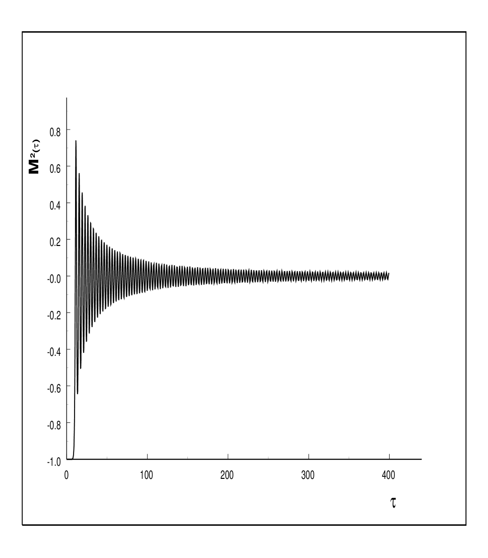
FIG. 1.: ${\cal M}^{2}(\tau)$ vs. $\tau$, $g=10^{-7}$

FIG. 2.: $g|\phi_{k}(\tau=100,200)|^{2}$ vs. $q=k/|m_{0}|$, $g=10^{-7}$

FIG. 3.: $gr\,C(r,\tau)$ vs $r/|m_{0}|$ for $t/|m_{0}|=100,\;200,\;300$ for $g=10^{-7}$.

FIG. 4.: $C^{2}(\eta)M^{2}(\eta)$ vs. $\eta$(conformal time in units of $m^{-1}_{0}$) for $\frac{T_{i}}{T_{c}}=3$, $g=10^{-5}$. R.D. Universe.

FIG. 5.: $\frac{\lambda}{2Nm^{2}_{0}}\langle\vec{\Phi}^{2}\rangle(\eta)$ vs. $\eta$ (conformal time in units of $m^{-1}_{0}$) for $\frac{T_{i}}{T_{c}}=3$, $g=10^{-5}$. R.D. Universe.

FIG. 6.: $\eta^{-5}|f_{k}(\eta)|^{2}$ vs. $k\eta$ for the same case as in Fig. 5.

FIG. 7.: $C(r,\eta)$ vs. $r$ for $\eta=250,400$ (in units of $m^{-1}_{0}$) for $\frac{T_{i}}{T_{c}}=3$, $g=10^{-5}$. R.D. FRW Universe.

REFERENCES

- [1] T. W. B. Kibble, J. Phys. A 9, 1387 (1976), and contribution to these proceedings.
- [2] M. B. Hindmarsh and T.W.B. Kibble, Rep. Prog. Phys. 58:477 (1995).
- [3] For a classification of topological defects in terms of the underlying group structure see T. Kibble’s contribution to these proceedings.
- [4] A. Vilenkin and E.P.S. Shellard, ‘Cosmic Strings and other Topological Defects’, Cambridge Monographs on Math. Phys. (Cambridge Univ. Press, 1994).
- [5] For a comprehensive review of the status of theory and experiment see: Proceedings of the ‘D. Chalonge’ School in Astrofundamental Physics at Erice, edited by N. Sánchez and A. Zichichi, 1996 World Scientific publisher and 1997, Kluwer Academic publishers. In particular the contributions by G. Smoot, A. N. Lasenby and A. Szalay., R. Durrer, M. Kunz and A. Melchiorri astro-ph/9811174, M. Kunz and R. Durrer, Phys. Rev. D55, R4516 (1997) and R. Durrer’s lectures in these proceedings.
- [6] See for example: K. Rajagopal in ‘Quark Gluon Plasma 2’, (Ed. R. C. Hwa, World Scientific, 1995).
- [7] A. J. Bray, Adv. Phys. 43, 357 (1994).
- [8] J. S. Langer in ‘Solids far from Equilibrium’, Ed. C. Godrèche, (Cambridge Univ. Press 1992); J. S. Langer in ‘Far from Equilibrium Phase Transitions’, Ed. L. Garrido, (Springer-Verlag, 1988); J. S. Langer in ‘Fluctuations, Instabilities and Phase Transitions’, Ed. T. Riste, Nato Advanced Study Institute, Geilo Norway, 1975 (Plenum, 1975).
- [9] G. Mazenko in in ‘Far from Equilibrium Phase Transitions’, Ed. L. Garrido, (Springer-Verlag, 1988).
- [10] C. Castellano and M. Zannetti, cond-mat/9807242; C. Castellano, F. Corberi and M. Zannetti, Phys. Rev. E56, 4973 (1997); F. Corberi, A. Coniglio and M. Zannetti, Phys. Rev. E51, 5469 (1995).
- [11] W. H. Zurek, Nature 317, 505 (1985); Acta Physica Polonica B24, 1301 1993); Phys. Rep. 276, (1996), see also W. H. Zurek’s contribution to these proceedings.
- [12] W. I. Goldburg and J. S. Huang, in ‘Fluctuations, Instabilities and Phase Transitions’, Ed. T. Riste, Nato Advanced Study Institute, Geilo Norway, 1975 (Plenum, 1975); J. S. Huang, W. I. Goldburg and M. R. Moldover, Phys. Rev. Lett. 34, 639 (1975).
- [13] N. Turok and D. N. Spergel, Phys. Rev. Lett. 66, 3093 (1991); D. N. Spergel, N. Turok, W. H. Press and B. S. Ryden, Phys. Rev. D43, 1038 (1991).
- [14] J. A. N. Filipe and A. J. Bray, Phys. Rev. E50, 2523 (1994); J. A. N. Filipe, (Ph. D. Thesis, 1994, unpublished).
- [15] D. Boyanovsky, H. J. de Vega and R. Holman, Phys. Rev. D 49, 2769 (1994); D. Boyanovsky, D. Cormier, H. J. de Vega, R. Holman et S. Prem Kumar, Phys. Rev. D57, 2166, (1998), (and references therein).
- [16] D. Boyanovsky, H. J. de Vega, R. Holman, D.-S. Lee and A. Singh, Phys. Rev. D51, 4419 (1995). D. Boyanovsky, H. J. de Vega and R. Holman, Proceedings of the Second Paris Cosmology Colloquium, Observatoire de Paris, June 1994, pp. 127-215, H. J. de Vega and N. Sánchez, Editors (World Scientific, 1995); Advances in Astrofundamental Physics, Erice Chalonge School, N. Sánchez and A. Zichichi Editors, (World Scientific, 1995). D. Boyanovsky, H. J. de Vega, R. Holman and J. Salgado, Phys. Rev. D54, 7570 (1996); D. Boyanovsky, D. Cormier, H. J. de Vega, R. Holman, A. Singh, M. Srednicki; Phys. Rev. D56 (1997) 1939. D. Boyanovsky, H. J. de Vega and R. Holman, Vth. Erice Chalonge School, Current Topics in Astrofundamental Physics, N. Sánchez and A. Zichichi Editors, World Scientific, 1996, p. 183-270. D. Boyanovsky, M. D’Attanasio, H. J. de Vega, R. Holman and D. S. Lee, Phys. Rev. D52, 6805 (1995). D. Boyanovsky, H. J. de Vega, R. Holman and J. Salgado, Phys. Rev. D57, 7388 (1998).
- [17] D. Boyanovsky, H. J. de Vega, R. Holman and J. Salgado, hep-ph/9811273, to appear in Phys. Rev. D.
- [18] F. Cooper, S. Habib, Y. Kluger, E. Mottola, Phys.Rev. D55 (1997), 6471. F. Cooper, S. Habib, Y. Kluger, E. Mottola, J. P. Paz, P. R. Anderson, Phys. Rev. D50, 2848 (1994). F. Cooper, Y. Kluger, E. Mottola, J. P. Paz, Phys. Rev. D51, 2377 (1995); F. Cooper and E. Mottola, Mod. Phys. Lett. A 2, 635 (1987); F. Cooper and E. Mottola, Phys. Rev. D36, 3114 (1987); F. Cooper, S.-Y. Pi and P. N. Stancioff, Phys. Rev. D34, 3831 (1986).
- [19] D. Boyanovsky, H. J. de Vega and R. Holman, in preparation.
- [20] L. F. Cugliandolo and D. S. Dean, J. Phys. A28, 4213 (1995); ibid L453, (1995); L. F. Cugliandolo, J. Kurchan and G. Parisi, J. Physique (France) 4, 1641 (1994) and L. Cugliandolo’s contribution to this School.
- [21] Relaxing the assumption of an instantaneous quench and allowing for a time dependence of the cooling mechanism has been recently studied by M. Bowick and A Momen, hep-ph/9803284.
- [22] E. J. Weinberg and A. Wu, Phys. Rev. D36, 2474 (1987); A. Guth and S.-Y. Pi, Phys. Rev. D32, 1899 (1985).
- [23] D. Boyanovsky and H. J. de Vega, Phys. Rev. D47, 2343 (1993); D. Boyanovsky Phys. Rev. E48, 767 (1993).
- [24] D. Boyanovsky, D.-S. Lee and A. Singh, Phys. Rev. D48, 800 (1993).
- [25] G. Karra and R.J.Rivers, Phys.Lett. B414 (1997), 28; R.J.Rivers, 3rd. Colloque Cosmologie, Observatoire de Paris, June 1995, p. 341 in the Proceedings edited by H J de Vega and N. Sánchez, World Scientific. A.J. Gill and R.J. Rivers, Phys.Rev. D51 (1995), 6949; G.J. Cheetham, E.J. Copeland, T.S. Evans, R.J. Rivers, Phys.Rev.D47 (1993),5316.
- [26] ‘Defect Formation and Critical Dynamics in the Early Universe’, G. J. Stephens, E. A. Calzetta, B. L. Hu, S. A. Ramsey, gr-qc/9808059 (1998). ‘Counting Defects in an Instantaneous Quench’, D. Ibaceta and E. Calzetta, hep-ph/9810301 (1998).