$NN$ interaction in a Goldstone boson exchange model

Abstract

Adiabatic nucleon-nucleon potentials are calculated in a six-quark nonrelativistic chiral constituent quark model where the Hamiltonian contains a linear confinement and a pseudoscalar meson (Goldstone boson) exchange interaction between quarks. Calculations are performed both in a cluster model and a molecular orbital basis, through coupled channels. In both cases the potentials present an important hard core at short distances, explained through the dominance of the $\displaystyle[51]_{FS}$ configuration, but do not exhibit an attractive pocket. We add a scalar meson exchange interaction and show how it can account for some middle-range attraction.

I Introduction

There have been many attempts to study the nucleon-nucleon interaction starting from a system of six interacting quarks described by a constituent quark model. These models explain the short range repulsion as due to the colour magnetic part of the one gluon exchange (OGE) interaction between quarks and due to quark interchanges between two $\displaystyle 3q$ clusters [1, 2]. To the OGE interaction it was necessary to add a scalar and a pseudoscalar meson exchange interaction between quarks of different $\displaystyle 3q$ clusters in order to explain the intermediate- and long-range attraction between two nucleons [3, 4, 5].

In a previous work [6] we have calculated the nucleon-nucleon ($\displaystyle NN$) interaction potential at zero-separation distance between two three-quark clusters in the frame of a constituent quark model [7, 8, 9] where the quarks interact via pseudoscalar meson i.e. Goldstone boson exchange (GBE) instead of OGE. An important motivation in using the GBE model is that it describes well the baryon spectra. In particular, it correctly reproduces the order of positive and negative parity states both for nonstrange [8] and strange [9] baryons where the OGE model has failed.

The underlying symmetry of the GBE model is related to the flavour-spin $\displaystyle SU_{F}(3)\times SU_{S}(2)$ group. Combining it with the $\displaystyle S_{3}$ symmetry, a thorough analysis performed for the $\displaystyle L=1$ baryons [10] has shown that the chiral quark picture leads to more satisfactory fits to the observed baryon spectrum than the OGE models.

The one-pion exchange potential between quarks appears naturally as an iteration of the instanton induced interaction in the t-channel [11]. The meson exchange picture is also supported by explicit QCD latice calculations [12].

Another motivation in using the GBE model is that the exchange interaction contains the basic ingredients required by the $\displaystyle NN$ problem. Its long-range part, required to provide the long-range $\displaystyle NN$ interaction, is a Yukawa-type potential depending on the mass of the exchange meson, Its short-range part, of opposite sign to the long-range one, is mainly responsible for the good description of the baryon spectra [7, 8, 9] and also induces a short-range repulsion in the $\displaystyle NN$ system, both in the ${}^{3}S_{1}$ and ${}^{1}S_{0}$ channels [13]. The present study is an extention of [6] and we calculate here the interaction potential between two $\displaystyle 3q$ clusters as a function of $\displaystyle Z$, the separation distance between the centres of the clusters. This separation distance is a good approximation of the Jacobi relative coordinate between the two clusters. Under this assumption, here we calculate the interaction potential in the adiabatic (Born-Oppenheimer) approximation, as explained below.

A common issue in solving the $\displaystyle NN$ problem is the construction of adequate six-quark basis states. The usual choice is a cluster model basis [1, 2, 14]. In calculating the potential at zero-separation distance, in Ref. [6] we used molecular-type orbitals [15] and compared the results with those based on cluster model single-particle states. The molecular orbitals have the proper axially and reflectionally symmetries and can be constructed from appropriate combinations of two-centre Gaussians. At zero-separation between the $\displaystyle 3q$ clusters the six-quark states obtained from such orbitals contain certain $\displaystyle p^{n}s^{6-n}$ configurations which are missing in the cluster model basis. By using molecular orbitals, in Ref. [6] we found that the height of the repulsion reduces by about 22 % and 25 % in the ${}^{3}S_{1}$ and ${}^{1}S_{0}$ channels respectively with respect to cluster model results. It is therefore useful to analyse the role of molecular orbitals at distances $\displaystyle Z\neq 0$. By construction, at $\displaystyle Z\rightarrow\infty$ the molecular orbital states are simple parity conserving linear combinations of cluster model states. Their role is expected to be important at short range at least. They also have the advantage of forming an orthogonal and complete basis while the cluster model (two-centre) states are not orthogonal and are overcomplete. For this reason we found that in practice they are more convenient to be used than the cluster model basis, where one must carefully [14] consider the limit $\displaystyle Z\rightarrow 0$. Here too, for the purpose of comparison we perform calculations both in the cluster model and the molecular orbital basis.

In Sec. 2 we recall the procedure of constructing molecular orbital single-particle states starting from the two-centre Gaussians used in the cluster model calculations. In Sec. 3 the GBE Hamiltonian is presented. Sec. 4 is devoted to the results obtained for the $\displaystyle NN$ potential. In Sec. 5 we introduce a middle range attraction through a scalar meson exchange interaction between quarks parametrized consistently with the pseudoscalar meson exchange. The last section is devoted to a summary and conclusions.

II The single-particle orbitals

In the cluster model one can define states which in the limit of large intercluster separation $\displaystyle Z$ are right $\displaystyle R$ and left $\displaystyle L$ states

$$R=\psi\left(\vec{r}-\frac{\vec{Z}}{2}\right)\hskip 22.76219pt\mbox{and}\hskip 22.76219ptL=\psi\left(\vec{r}+\frac{\vec{Z}}{2}\right).$$ (1)

In the simplest cluster model basis these are ground state harmonic oscillator wave functions centered at $\displaystyle Z/2$ and $\displaystyle-Z/2$ respectively. They contain a parameter $\displaystyle\beta$ which is fixed variationally to minimize the nucleon mass described as a $\displaystyle 3q$ cluster within a given Hamiltonian. The states (1) are normalized but are not orthogonal at finite $\displaystyle Z$. They have good parity about their centers but not about their common center $\displaystyle\vec{r}=0$.

From $\displaystyle R$ and $\displaystyle L$ one constructs six-quark states of given orbital symmetry $\displaystyle[f]_{O}$. The totally antisymmetric six-quark states also contain a flavour-spin part of symmetry $\displaystyle[f]_{FS}$ and a colour part of symmetry $\displaystyle[222]_{C}$. In the cluster model the most important basis states [13] for the Hamiltonian described in the following section are

$$\left|{\left.{{R}^{3}{L}^{3}\ {\left[{6}\right]}_{O}\ {\left[{33}\right]}_{FS}}\right\rangle}\right.$$ (2)

$$\left|{\left.{{R}^{3}{L}^{3}\ {\left[{42}\right]}_{O}\ {\left[{33}\right]}_{FS}}\right\rangle}\right.$$ (3)

$$\left|{\left.{{R}^{3}{L}^{3}\ {\left[{42}\right]}_{O}\ {\left[{51}\right]}_{FS}}\right\rangle}\right.$$ (4)

$$\left|{\left.{{R}^{3}{L}^{3}\ {\left[{42}\right]}_{O}\ {\left[{411}\right]}_{FS}}\right\rangle}\right.$$ (5)

Harvey [14] has shown that with a proper normalization the symmetry $\displaystyle[6]_{O}$ contains only $\displaystyle s^{6}$ and $\displaystyle[42]_{O}$ only $\displaystyle s^{4}p^{2}$ configurations in the limit $\displaystyle Z\rightarrow 0$.

According to Ref. [15] let us consider now molecular orbital single-particle states. Most generally these are eigenstates of a Hamiltonian $\displaystyle H_{0}$ having axial and reflectional symmetries characteristic to the $\displaystyle NN$ problem. These eigenstates have therefore good parity and good angular momentum projection. As in the cluster model basis where one uses the two lowest states $\displaystyle R$ and $\displaystyle L$, in the molecular orbital basis we also consider the two lowest states, $\displaystyle\sigma$, of positive parity and $\displaystyle\pi$, of negative parity. From these we can construct pseudo-right $\displaystyle r$ and pseudo-left $\displaystyle l$ states as

$$\left[\begin{array}[]{c}r\\ l\end{array}\right]=2^{-1/2}\,(\sigma\pm\pi)\hskip 14.22636pt\rm{for\ all\ }Z,$$ (6)

where

$$\displaystyle<r|r>=<l|l>=1,\,\,<r|l>=0.$$ (7)

In principle one can obtain molecular orbital single particle states from mean field calculations (see for example [16]). Here we approximate them by good parity, orthonormal states constructed from the cluster model states (1) as

$$\left[\begin{array}[]{c}\sigma\\ \pi\end{array}\right]=[2(1\pm<R|L>)]^{-1/2}(R\pm L),$$ (8)

Such molecular orbitals are a very good approximation to the exact eigenstates of a “two-centre” oscillator frequently used in nuclear physics or occasionally [17] in the calculation of the $\displaystyle NN$ potential. They provide a convenient basis for the first step calculations based on the adiabatic approximation as described below.

Introduced in (6) they give

$$\left[\begin{array}[]{c}r\\ l\end{array}\right]=\frac{1}{2}\left[\frac{R+L}{(1+<R|L>)^{1/2}}\pm\frac{R-L}{(1-<R|L>)^{1/2}}\right].$$ (9)

At $\displaystyle Z\rightarrow 0$ one has $\displaystyle\sigma\rightarrow s$ and $\displaystyle\pi\rightarrow p$ (with $\displaystyle m=0,\pm 1$) where $\displaystyle s$ and $\displaystyle p$ are harmonic oscillator states. Thus in the limit $\displaystyle Z\rightarrow 0$ one has

$$\left[\begin{array}[]{c}r\\ l\end{array}\right]=2^{1/2}(s\pm p),$$ (10)

and at $\displaystyle Z\rightarrow\infty$ one recovers the cluster model basis because $\displaystyle r\rightarrow R$ and $\displaystyle\ell\rightarrow L$.

Equation (9) with $\displaystyle R$ and $\displaystyle L$ defined by (1) ensures that the same $\displaystyle Z$ is used both in the molecular and the cluster model basis.

From $\displaystyle(r,l)$ as well as from $\displaystyle(\sigma,\pi)$ orbitals one can construct six-quark states of required permutation symmetry. For the $\displaystyle S_{6}$ symmetries relevant for the $\displaystyle NN$ problem the transformations between six-quark states expressed in terms of $\displaystyle(r,l)$ and $\displaystyle(\sigma,\pi)$ states are given in Table I of Ref. [15]. This table shows that in the limit $\displaystyle Z\rightarrow 0$ six-quark states obtained from molecular orbitals contain configurations of type $\displaystyle s^{n}p^{6-n}$ with $\displaystyle n=0,1,...,6$. For example the $\displaystyle[6]_{O}$ state contains $\displaystyle s^{6}$, $\displaystyle s^{6}p^{4}$, $\displaystyle s^{2}p^{4}$ and $\displaystyle p^{6}$ configurations and the $\displaystyle[42]_{O}$ state associated to the $\displaystyle S$-channel contains $\displaystyle s^{4}p^{2}$ and $\displaystyle s^{2}p^{4}$ configurations. This is in contrast to the cluster model basis where $\displaystyle[6]_{O}$ contains only $\displaystyle s^{6}$ and $\displaystyle[42]_{O}$ only $\displaystyle s^{4}p^{2}$ configurations, as mentioned above. This suggests that the six-quark basis states constructed from molecular orbitals form a richer basis without introducing more single particle states.

Using Table I of Ref. [15] we find that the six-quark basis states needed for the ${}^{3}S_{1}$ or ${}^{1}S_{0}$ channels are:

$$\displaystyle\left.{\left|{33{\left[{6}\right]}_{O}{\left[{33}\right]}_{FS}}\right.}\right\rangle\ \displaystyle= \displaystyle\frac{1}{4}\ \left.{\left|\left[{\sqrt{5}\ \left({{\sigma}^{6}\ -\ {\pi}^{6}}\right)\ -\ \sqrt{3}\ \left({{\sigma}^{4}{\pi}^{2}\ -\ {\sigma}^{2}{\pi}^{4}}\right)}\right]\ {{\left[{6}\right]}_{O}{\left[{33}\right]}_{FS}}\right.}\right\rangle,$$ (11)

$$\displaystyle\left.{\left|{33{\left[{42}\right]}_{O}{\left[{33}\right]}_{FS}}\right.}\right\rangle\ \displaystyle= \displaystyle\sqrt{\frac{1}{2}}\ \left.{\left|{\left[{{\sigma}^{4}{\pi}^{2}\ -\ {\sigma}^{2}{\pi}^{4}}\right]{\left[{42}\right]}_{O}{\left[{33}\right]}_{FS}}\right.}\right\rangle,$$ (12)

$$\displaystyle\left.{\left|{33{\left[{42}\right]}_{O}{\left[{51}\right]}_{FS}}\right.}\right\rangle\ \displaystyle= \displaystyle\sqrt{\frac{1}{2}}\ \left.{\left|{\left[{{\sigma}^{4}{\pi}^{2}\ -\ {\sigma}^{2}{\pi}^{4}}\right]{\left[{42}\right]}_{O}{\left[{51}\right]}_{FS}}\right.}\right\rangle,$$ (13)

$$\displaystyle\left.{\left|{33{\left[{42}\right]}_{O}{\left[{411}\right]}_{FS}}\right.}\right\rangle\ \displaystyle= \displaystyle\sqrt{\frac{1}{2}}\ \left.{\left|{\left[{{\sigma}^{4}{\pi}^{2}\ -\ {\sigma}^{2}{\pi}^{4}}\right]{\left[{42}\right]}_{O}{\left[{411}\right]}_{FS}}\right.}\right\rangle,$$ (14)

$$\displaystyle\left.{\left|{{42}^{+}{\left[{6}\right]}_{O}{\left[{33}\right]}_{FS}}\right.}\right\rangle\ \displaystyle= \displaystyle{\frac{1}{4}}\sqrt{{\frac{1}{2}}}\ \left.{\left|{\left[{{\sqrt{15}}\left({{\sigma}^{6}\ +\ {\pi}^{6}}\right)\ -\ \left({{\sigma}^{4}{\pi}^{2}\ +\ {\sigma}^{2}{\pi}^{4}}\right)}\right]{\left[{6}\right]}_{O}{\left[{33}\right]}_{FS}}\right.}\right\rangle,$$ (15)

$$\displaystyle\left.{\left|{{42}^{+}{\left[{42}\right]}_{O}{\left[{33}\right]}_{FS}}\right.}\right\rangle\ \displaystyle= \displaystyle\sqrt{\frac{1}{2}}\ \left.{\left|{\left[{\left.{{\sigma}^{4}{\pi}^{2}}\right.\ +\ {\sigma}^{2}{\pi}^{4}}\right]{\left[{42}\right]}_{O}{\left[{33}\right]}_{FS}}\right.}\right\rangle,$$ (16)

$$\displaystyle\left.{\left|{{42}^{+}{\left[{42}\right]}_{O}{\left[{51}\right]}_{FS}}\right.}\right\rangle\ \displaystyle= \displaystyle\sqrt{\frac{1}{2}}\ \left.{\left|{\left[{\left.{{\sigma}^{4}{\pi}^{2}}\right.\ +\ {\sigma}^{2}{\pi}^{4}}\right]{\left[{42}\right]}_{O}{\left[{51}\right]}_{FS}}\right.}\right\rangle,$$ (17)

$$\displaystyle\left.{\left|{{42}^{+}{\left[{42}\right]}_{O}{\left[{411}\right]}_{FS}}\right.}\right\rangle\ \displaystyle= \displaystyle\sqrt{\frac{1}{2}}\ \left.{\left|{\left[{\left.{{\sigma}^{4}{\pi}^{2}}\right.\ +\ {\sigma}^{2}{\pi}^{4}}\right]{\left[{42}\right]}_{O}{\left[{411}\right]}_{FS}}\right.}\right\rangle,$$ (18)

$$\displaystyle\left.{\left|{{51}^{+}{\left[{6}\right]}_{O}{\left[{33}\right]}_{FS}}\right.}\right\rangle\ \displaystyle= \displaystyle\frac{1}{4}\ \left.{\left|{\left[{\sqrt{3}\ \left.{\left({{\sigma}^{6}\ -\ {\pi}^{6}}\right)}\right.\ +\ \sqrt{5}\ \left({{\sigma}^{4}{\pi}^{2}\ -\ {\sigma}^{2}{\pi}^{4}}\right)}\right]{\left[{6}\right]}_{O}{\left[{33}\right]}_{FS}}\right.}\right\rangle,$$ (19)

where the notation $\displaystyle 33$ and $\displaystyle mn^{+}$ in the left-hand side of each equality above means $\displaystyle r^{3}\ell^{3}$ and $\displaystyle r^{m}\ell^{n}+r^{n}\ell^{m}$ as in Ref. [15]. Each wave function contains an orbital part ($\displaystyle O$) and a flavour-spin part ($\displaystyle FS$) which combined with the colour singlet $\displaystyle[222]_{C}$ state gives rise to a totally antisymmetric state. We restricted the flavour-spin states to $\displaystyle[33]_{FS}$, $\displaystyle[51]_{FS}$ and $\displaystyle[411]_{FS}$ as for the cluster model basis (2-5).

As explained above, besides being poorer in $\displaystyle s^{n}p^{6-n}$ configurations, the number of basis states is smaller in the cluster model although we deal with the same $\displaystyle[f]_{O}$ and $\displaystyle[f]_{FS}$ symmetries and the same harmonic oscillator states $\displaystyle s$ and $\displaystyle p$ in both cases. This is due to the existence of three-quark clusters only in the cluster model states, while the molecular basis also allows configurations with five quarks to the left and one to the right, or vice versa, or four quarks to the left and two to the right or vice versa. At large separations these states act as “hidden colour” states but at short- and medium-range separation distances they are expected to bring a significant contribution, as we shall see below. The ”hidden colour” are states where a $\displaystyle 3q$ cluster in an $\displaystyle s^{3}$ configuration is a colour octet, in contrast to the nucleon which is a colour singlet. Their role is important at short separations but it vanishes at large ones (see e.g. [14]).

III Hamiltonian

The GBE Hamiltonian considered in this study has the form [8, 9] :

$$H=\sum_{i}m_{i}+\sum_{i}\frac{\vec{p}_{i}^{\,2}}{2m_{i}}-\frac{(\sum_{i}\vec{p}_{i})^{2}}{2\sum_{i}m_{i}}+\sum_{i<j}V_{\text{conf}}(r_{ij})+\sum_{i<j}V_{\chi}(r_{ij})\,,$$ (20)

with the linear confining interaction :

$$V_{\text{conf}}(r_{ij})=-\frac{3}{8}\lambda_{i}^{c}\cdot\lambda_{j}^{c}\,(V_{0}+C\,r_{ij}\,),$$ (21)

and the spin–spin component of the GBE interaction in its $\displaystyle SU_{F}(3)$ form :

$$\displaystyle V_{\chi}(r_{ij}) \displaystyle= \displaystyle\left\{\sum_{F=1}^{3}V_{\pi}(r_{ij})\lambda_{i}^{F}\lambda_{j}^{F}\right.$$ (22)

$$\displaystyle+ \displaystyle\left.\sum_{F=4}^{7}V_{K}(r_{ij})\lambda_{i}^{F}\lambda_{j}^{F}+V_{\eta}(r_{ij})\lambda_{i}^{8}\lambda_{j}^{8}+V_{\eta^{\prime}}(r_{ij})\lambda_{i}^{0}\lambda_{j}^{0}\right\}\vec{\sigma}_{i}\cdot\vec{\sigma}_{j},$$ (23)

with $\displaystyle\lambda^{0}=\sqrt{2/3}~{}{\bf 1}$, where $\displaystyle\bf 1$ is the $\displaystyle 3\times 3$ unit matrix. The interaction (22) contains $\displaystyle\gamma=\pi,K,\eta$ and $\displaystyle\eta^{\prime}$ meson-exchange terms and the form of $\displaystyle V_{\gamma}\left(r_{ij}\right)$ is given as the sum of two distinct contributions : a Yukawa-type potential containing the mass of the exchanged meson and a short-range contribution of opposite sign, the role of which is crucial in baryon spectroscopy.

In the parametrization of Ref. [8] the exchange potential due to a meson $\displaystyle\gamma$ has the form

$$V_{\gamma}(r)=\frac{g_{\gamma}^{2}}{4\pi}\frac{1}{12m_{i}m_{j}}\{\theta(r-r_{0})\mu_{\gamma}^{2}\,\frac{e^{-\mu_{\gamma}r}}{r}-\frac{4}{\sqrt{\pi}}\alpha^{3}\exp(-\alpha^{2}(r-r_{0})^{2})\}.$$ (24)

The shifted Gaussian of Eq. (23) results from a pure phenomenological fit (see below) of the baryon spectrum with

$$r_{0}=0.43\,{fm},~{}\alpha=2.91\,{fm}^{-1},~{}~{}$$ (25)

For a system of $\displaystyle u$ and $\displaystyle d$ quarks only, as it is the case here, the $\displaystyle K$-exchange does not contribute. The apriori determined parameters of the GBE model are the masses

$$m_{u,d}=340\,{MeV},\,\mu_{\pi}=139\,{MeV},~{}\mu_{\eta}=547\,{MeV},~{}\mu_{\eta^{\prime}}=958\,{MeV}.$$ (26)

The other parameters are given in Table I.

It is useful to comment on Eq. (23). The coupling of pseudoscalar mesons to quarks (or nucleons) gives rise to a two-body interaction potential which contains a Yukawa-type term and a contact term of opposite sign (see e.g. [18]). The second term of (23) stems from the contact term, regularized with parameters fixed phenomenologically. Certainly more fundamental studies are required to understand this second term and attempts are being made in this direction. The instanton liquid model of the vacuum (for a review see [19]) implies point-like quark-quark interactions. To obtain a realistic description of the hyperfine interaction this interaction has to be iterated in the t-channel [11]. The t-channel iteration admits a meson exchange interpretation [20].

In principle it would be better to use a parametrization of the GBE interaction as given in [21] based on a semirelativistic Hamiltonian. However, in applying the quark cluster approach to two-baryon systems we are restricted to use a nonrelativistic kinematics and an $\displaystyle s^{3}$ wave function for the ground state baryon.

The matrix elements of the Hamiltonian (20) are calculated in the bases (2)-(5) and (11)-(19) by using the fractional parentage technique described in Refs. [14, 22] and also applied in Ref. [13]. A programme based on Mathematica [23] has been created for this purpose. In this way every six-body matrix element reduces to a linear combination of two-body matrix elements of either symmetric or antisymmetric states for which Eqs. (3.3) of Ref. [7] can be used to integrate in the flavour-spin space.

IV Results

We diagonalize the Hamiltonian (20)-(25) in the six-quark cluster model basis (2)-(5) and in the six-quark molecular orbital basis (11)-(19) for values of the separation distance $\displaystyle Z$ up to 2.5 fm. Using in each case the lowest eigenvalue, denoted by $\displaystyle\langle H\rangle_{Z}$ we define the $\displaystyle NN$ interaction potential in the adiabatic (Born-Oppenheimer) approximation as

$$V_{NN}\left(Z\right)=\langle H\rangle_{Z}-2m_{N}-K_{rel}$$ (27)

Here $\displaystyle m_{N}$ is the nucleon mass obtained as a variational $\displaystyle s^{3}$ solution for a $\displaystyle 3q$ system described by the Hamiltonian (20). The wavefunction has the form $\displaystyle\phi\ \propto\ \exp\ \ \left[{-\ \left({{\rho}^{2}\ +\ {\lambda}^{2}}\right)/2{\beta}^{2}}\right]$ where $\displaystyle\rho=\left(\vec{r}_{1}-\vec{r}_{2}\right)/\sqrt{2}$ and $\displaystyle\vec{\lambda}=\left(\vec{r}_{1}+\vec{r}_{2}-2\vec{r}_{3}\right)/\sqrt{6}$. The variational solution for $\displaystyle m_{N}=\langle H\rangle_{3q}$ and the corresponding $\displaystyle\beta$ is given in Table II. The same value of $\displaystyle\beta$ is also used for the 6q system. This is equivalent with imposing the “stability condition” which is of crucial importance in resonating group method (RGM) calculations [1, 2]. The quantity $\displaystyle K_{rel}$ represents the relative kinetic energy of two $\displaystyle 3q$ clusters separated at infinity

$${K}_{rel}\ =\ {\frac{{3\hbar}^{2}}{4{m\beta}^{2}}}\$$ (28)

where $\displaystyle m$ above and in the following designates the mass of the $\displaystyle u$ or $\displaystyle d$ quark. For the value of $\displaystyle\beta$ of Table II this gives $\displaystyle K_{rel}=0.448$ GeV.

A Cluster model

In Fig. 1 we present the expectation value of the kinetic energy $\displaystyle\langle KE\rangle$ as a function of $\displaystyle Z$. One can see that for the state $\displaystyle\left|{\left.{{R}^{3}{L}^{3}{\left[{42}\right]}_{O}}\right\rangle}\right.$ it decreases with $\displaystyle Z$ but for the state $\displaystyle\left|{\left.{{R}^{3}{L}^{3}{\left[{6}\right]}_{O}}\right\rangle}\right.$ it first reaches a minimum at around $\displaystyle Z\cong$ 0.85 fm and then tends to an asymptotic value equal to its value at the origin due to its $\displaystyle s^{6}$ structure. This value is

$$\langle KE\rangle_{Z=0}=\langle KE\rangle_{Z=\infty}=\frac{15}{4}\hbar\omega$$ (29)

where $\displaystyle\hbar\omega=\hbar^{2}/m\beta^{2}$. Actually this is also the asymptotic value for all states.

The diagonal matrix elements of the confinement potential are presented in Fig. 2. Beyond $\displaystyle Z>$ 1.5 fm one can notice a linear increase except for the $\displaystyle\left|{\left.{{R}^{3}{L}^{3}{\left[{42}\right]}_{O}{\left[{51}\right]}_{FS}}\right\rangle}\right.$ state where it reaches a plateau of 0.3905 GeV.

As an example the diagonal matrix elements of the chiral interaction $\displaystyle V_{\chi}$ are exhibited in Fig. 3 for $\displaystyle S=1$, $\displaystyle I=0$. At $\displaystyle Z=0$ one recovers the values obtained in Ref. [6]. At $\displaystyle Z\rightarrow\infty$ the symmetries corresponding to baryon-baryon channels, namely $\displaystyle[51]_{FS}$ and $\displaystyle[33]_{FS}$, must appear with proper coefficients, as given by Eq. (29). The contribution due to these symmetries must be identical to the contribution of $\displaystyle V_{\chi}$ to two nucleon masses also calculated with the Hamiltonian (20). This is indeed the case. In the total Hamiltonian the contribution of the $\displaystyle[411]_{FS}$ $\displaystyle V_{\chi}$ state tends to infinity when $\displaystyle Z\rightarrow\infty$. Then this state decouples from the rest which is natural because it does not correspond to an asymptotic baryon-baryon channel. It plays a role at small $\displaystyle Z$ but at large $\displaystyle Z$ its amplitude in the $\displaystyle NN$ wavefunction vanishes, similarly to the “hidden colour” states. Actually, in diagonalizing the total Hamiltonian in the basis (2)-(5) we obtain an $\displaystyle NN$ wavefunction which in the limit $\displaystyle Z\rightarrow\infty$ becomes [14]

$${\psi}_{NN}\ =\ {\frac{1}{3}}\ \left|{\left.{{\left[{6}\right]}_{O}{\left[{33}\right]}_{FS}}\right\rangle}\right.\ +\ {\frac{2}{3}}\ \left|{\left.{{\left[{42}\right]}_{O}{\left[{33}\right]}_{FS}}\right\rangle}\right.\ -\ {\frac{2}{3}}\ \left|{\left.{{\left[{42}\right]}_{O}{\left[{51}\right]}_{FS}}\right\rangle}\right.$$ (30)

The adiabatic potential drawn in Figs. 6 and 7 is defined according to Eq. (26) where $\displaystyle\langle H\rangle_{Z}$ is the lowest eigenvalue resulting from the diagonalization. Fig. 6 corresponds to $\displaystyle S$ = 1, $\displaystyle I$ = 0 and Fig. 7 to $\displaystyle S$ = 0, $\displaystyle I$=1. Note that from these curves one should subtract $\displaystyle K_{rel}$ of Eq. (27) in order to obtain the asymptotic value zero for the potential. One can see that the potential is repulsive at any $\displaystyle Z$ in both sectors.

Our cluster model results can be compared to previous literature based on OGE models. A typical example for the ${}^{3}S_{1}$ and ${}^{1}S_{0}$ adiabatic potentials can be found in Ref.[24]. The results are similar to ours. There is a repulsive core but no attractive pocket. However, in our case, in either bases, the core is about twice higher at $\displaystyle Z$ = 0 and about 0.5 fm wider than in [24].

B Molecular orbital basis

In the molecular basis the diagonal matrix elements of the kinetic energy are similar to each other as decreasing functions of $\displaystyle Z$. As an illustration in Fig. 4 we show $\displaystyle\langle K.E.\rangle$ corresponding to $\displaystyle\left|{\left.{33{\left[{6}\right]}_{O}{\left[{33}\right]}_{FS}}\right\rangle}\right.$ and to the most dominant state at $\displaystyle Z=0$, namely $\displaystyle\left|{\left.{42^{+}{\left[{42}\right]}_{O}{\left[{51}\right]}_{FS}}\right\rangle}\right.$ (see [6]). The kinetic energy of the latter is larger than that of the former because of the presence of the configuration $\displaystyle s^{2}p^{4}$ with 50 % probability while in the first state this probability is smaller as well as that of the $\displaystyle p^{6}$ configuration, see eqs. (11) and (17). The large kinetic energy of the state (17) is compensated by large negative values of $\displaystyle\langle V_{\chi}\rangle$ so that this state becomes dominant at small $\displaystyle Z$ in agreement with Ref. [6].

The expectation values of the confinement potential increase with $\displaystyle Z$ becoming linear beyond $\displaystyle Z>$ 1.5 fm except for the state $\displaystyle\left|{\left.{33{\left[{42}\right]}_{O}{\left[{51}\right]}_{FS}}\right\rangle}\right.$ which gives a result very much similar to the cluster model state $\displaystyle\left|{\left.{R^{3}L^{3}{\left[{42}\right]}_{O}{\left[{51}\right]}_{FS}}\right\rangle}\right.$ drawn in Fig. 2. Such a behaviour can be understood through the details given in the Appendix. Due to the similarity to the cluster model results we do not show here $\displaystyle\langle V_{conf}\rangle$ explicitly for the molecular orbital basis.

The expectation value of the chiral interaction either decreases or increases with $\displaystyle Z$ depending on the state. In Fig. 5 we illustrate the case of the $\displaystyle\left|{\left.{42^{+}{\left[{42}\right]}_{O}{\left[{51}\right]}_{FS}}\right\rangle}\right.$ state. both for $\displaystyle S$ = 1, $\displaystyle I$ = 0 and $\displaystyle S$ = 0, $\displaystyle I$ = 1 sectors. This state is the dominant component of $\displaystyle{\psi}_{NN}$ at $\displaystyle Z$ = 0 with a probability of 87 % for $\displaystyle SI$ = (10) and 93 % for $\displaystyle SI$ = (01) [6]. With increasing $\displaystyle Z$ these probabilities decrease and tend to zero at $\displaystyle Z\rightarrow\infty$. In fact in the molecular orbital basis the asymptotic form of $\displaystyle{\psi}_{NN}$ is also given by Eq. (29) inasmuch as $\displaystyle r\rightarrow R$ and $\displaystyle l\rightarrow L$ as indicated below Eq. (10).

Adding together these contributions we diagonalize the Hamiltonian and use its lowest eigenvalue to obtain the $\displaystyle NN$ potential according to the definition (26). The $\displaystyle S=1$, $\displaystyle I=0$ and $\displaystyle S=0$, $\displaystyle I=1$ cases are illustrated in Figs. 6 and 7 respectively, for a comparison with the cluster model basis. As shown in Ref. [6] at $\displaystyle Z=0$ the repulsion reduces by about 22 % and 25 % in the ${}^{3}S_{1}$ and ${}^{1}S_{0}$ channels respectively when passing from the cluster model basis to the molecular orbital basis. From Figs. 6 and 7 one can see that the molecular orbital basis has an important effect up to about $\displaystyle Z\approx$ 1.5 fm giving a lower potential at small values of $\displaystyle Z$. For $\displaystyle Z\approx 1$ fm it gives a potential larger by few tens of MeV than the cluster model potential. However there is no attraction at all in either case.

Actually, by construction, the molecular orbital basis is richer at $\displaystyle Z$ = 0 [15] than the cluster model basis. For this reason, at small $\displaystyle Z$ it leads to a lower potential than the cluster model basis. Within a truncated space this property may not hold beyond some value of $\displaystyle Z$. However by an increase of the Hilbert space one can possibly bring the molecular potential lower again. In fact we chose the most important configurations from symmetry arguments [13] based on Casimir operator eigenvalues. These arguments hold if the interaction is the same for all quarks in the coordinate space. This is certainly a better approximation for $\displaystyle Z$ = 0 than for larger values of $\displaystyle Z$. So it means that other configurations, which have been neglected, may play a role at $\displaystyle Z>0.4$ fm. Then, if added, they could possibly lower the molecular basis result.

As defined in Sec. 2 the quantity $\displaystyle Z$ is the separation distance between two $\displaystyle 3q$ clusters. It represents the Jacobi relative coordinate between the two nucleons only for large $\displaystyle Z$. There we view it as a generator coordinate and the potential we obtain represents the diagonal kernel appearing in the resonating group or the generator coordinate method. The comparison given above should then be considered in the context of the generator coordinate method wich will be developped in further studies and will lead to nonlocal potentials. However the adiabatic potentials, here obtained in the two bases can be compared with each other in an independent and different way. On can introduce the quadrupole moment of the six-quark system

$$q_{20}=\sum_{i=1}^{6}r_{i}^{2}\ Y_{20}(\hat{r}_{i})$$ (31)

and treat the square root of its expectation value

$$\langle Q\rangle=\langle\psi_{NN}|q_{20}|\psi_{NN}\rangle$$ (32)

as a collective coordinate describing the separation between the two nucleons. Obviously $\displaystyle\sqrt{\langle Q\rangle}\rightarrow Z$ for large $\displaystyle Z$.

In Fig. 8 we plot $\displaystyle\sqrt{\langle Q\rangle}$ as a function of $\displaystyle Z$. The results are practically identical for $\displaystyle IS$ = (01) and $\displaystyle IS$ = (10). Note that $\displaystyle\sqrt{\langle Q\rangle}$ is normalized such as to be identical to $\displaystyle Z$ at large $\displaystyle Z$. One can see that the cluster model gives $\displaystyle\sqrt{\langle Q\rangle}=0$ at $\displaystyle Z=0$, consistent with the spherical symmetry of the system, while the molecular basis result is $\displaystyle\sqrt{\langle Q\rangle}=0.573$ fm at $\displaystyle Z=0$, wich suggests that the system acquires a small deformation in the molecular basis. This also means that its r.m.s. radius is larger in the molecular basis.

In Figs. 9 and 10 we plot the adiabatic potentials as a function of $\displaystyle\sqrt{\langle Q\rangle}$ instead of $\displaystyle Z$, for $\displaystyle IS$ = (01) and (10) respectively. As $\displaystyle\sqrt{\langle Q\rangle}\neq 0$ at any $\displaystyle Z$ in the molecular orbital basis, the corresponding potential is shifted to the right and appears above the cluster model potential at finite values of $\displaystyle\sqrt{\langle Q\rangle}$ but tends asymptotically to the same value. The comparison made in Figs. 9 and 10 is meaningful in the context of a Schrödinger type equation where the local adiabatic potential appears in conjunction with an “effective mass” depending on $\displaystyle\sqrt{\langle Q\rangle}$ also. However an effective mass can be obtain through RGM calculations and our future plan is to perform such calculations.

V The middle range attraction

In principle we expected some attraction at large $\displaystyle Z$ due to the presence of the Yukawa potential tail in Eq. (23). To see the net contribution of this part of the quark-quark interaction we repeated the calculations in the molecular orbital basis by completely removing the first term - the Yukawa potential part - in Eq. (23). The result is shown in Fig. 11. for $\displaystyle SI$= (10). One can see that beyond $\displaystyle Z\approx 1.3$ fm the contribution of the Yukawa potential tail is very small, of the order of 1-2 MeV. At small values of $\displaystyle Z$ the Yukawa part of (23) contributes to increase the adiabatic potential because it diminishes the attraction in the two body matrix elements.

The missing medium- and long-range attraction can in principle be simulated in a simple phenomenological way. For example, in Ref. [1] this has been achieved at the baryon level. Here we adopt a more consistent procedure assuming that besides the pseudoscalar meson exchange interaction of Sec. III there exists an additional scalar, $\displaystyle\sigma$-meson exchange interaction between quarks. This is in the spirit of the spontaneous chiral symmetry breaking mechanism on which the GBE model is based. The $\displaystyle\sigma$-meson is the chiral partner of the pion and it should be considered explicitly.

Actually once the one-pion exchange interaction between quarks is admitted, one can inquire about the role of at least two-pion exchanges. Recently it was found [20] that the two-pion exchange also plays a significant role in the quark-quark interaction. It enhances the effect of the isospin dependent spin-spin component of the one-pion exchange interaction and cancels out its tensor component. Apart from that it gives rise to a spin independent central component, which averaged over the isospin wave function of the nucleon it produces an attractive spin independent interaction. These findings also support the introduction of a scalar ($\displaystyle\sigma$-meson) exchange interaction between quarks as an approximate description of the two-pion exchange loops.

For consistency with the parametrization [8] we consider here a scalar quark-quark interaction of the form

$$V_{\sigma}(r)=\frac{g_{\sigma}^{2}}{4\pi}\frac{1}{12m_{i}m_{j}}\{\theta(r-r^{\prime}_{0})\mu_{\sigma}^{2}\,\frac{e^{-\mu_{\sigma}r}}{r}-\frac{4}{\sqrt{\pi}}\alpha^{\prime 3}\exp(-\alpha^{\prime 2}(r-r^{\prime}_{0})^{2})\}.$$ (33)

where $\displaystyle\mu_{\sigma}$ = 675 MeV and $\displaystyle r^{\prime}_{0}$, $\displaystyle\alpha^{\prime}$ and the coupling constant $\displaystyle g^{2}_{\sigma}/4\pi$ are arbitrary parameters. In order to be effective at medium-range separation between nucleons we expect this interaction to have $\displaystyle r^{\prime}_{0}\neq r_{0}$ and $\displaystyle\alpha^{\prime}\neq\alpha$. Note that the factor $\displaystyle 1/m_{i}m_{j}$ has only been introduced for dimensional reasons.

We first looked at the baryon spectrum with the same variational parameters as before. The only modification is a shift of the whole spectrum which would correspond to taking $\displaystyle V_{0}\approx-60$ MeV in Eq. (21).

For the $\displaystyle 6q$ system we performed calculations in the molecular basis, which is more appropriate than the cluster model basis. We found that the resulting adiabatic potential is practically insensitive to changes in $\displaystyle\mu_{\sigma}$ and $\displaystyle r^{\prime}_{0}$ but very sensitive to $\displaystyle\alpha^{\prime}$. In Fig. 12 we show results for

$$r^{\prime}_{0}=0.86\,{fm},~{}\alpha^{\prime}=1.47\,{fm}^{-1},~{}~{}g^{2}_{\sigma}/4\pi=g^{2}_{8}/4\pi$$ (34)

One can see that $\displaystyle V_{\sigma}$ produces indeed an attractive pocket, deeper for $\displaystyle SI$ = (10) than for (01), as it should be for the $\displaystyle NN$ problem. The depth of the attraction depends essentially on $\displaystyle\alpha^{\prime}$. The precise values of the parameters entering Eq. (32) should be determined in further RGM calculations. As mentioned above the Born-Oppenheimer potential is in fact the diagonal RGM kernel. It is interesting that an attractive pocket is seen in this kernel when a $\displaystyle\sigma$-meson exchange interaction is combined with pseudoscalar meson exchange and OGE interactions (hybrid model), the whole being fitted to the $\displaystyle NN$ problem [25].

VI Summary

We have calculated the $\displaystyle NN$ potential in the adiabatic approximation as a function of $\displaystyle Z$, the separation distance between the centres of the two $\displaystyle 3q$ clusters. We used a constituent quark model where quarks interact via pseudoscalar meson exchange. The orbital part of the six-quark states was constructed either from cluster model or molecular orbital single particle states. The latter are more realistic, having the proper axially and reflectionally symmetries. Also technically they are more convenient. We explicitly showed that they are important at small values of $\displaystyle Z$. In particular we found that the $\displaystyle NN$ potential obtained in the molecular orbital basis has a less repulsive core than the one obtained in the cluster model basis. However none of the bases leads to an attractive pocket. We have simulated this attraction by introducing a $\displaystyle\sigma$-meson exchange interaction between quarks.

To have a better understanding of the two bases we have also calculated the quadrupole mement of the $\displaystyle 6q$ system as a function of $\displaystyle Z$. The results show that in the molecular orbital basis the system acquires some small deformation at $\displaystyle Z=0$. As a function of the quadrupole moment the adiabatic potential looks more repulsive in the molecular orbital basis then in the cluster model basis. In this light one might naively expect that the molecular basis will lead to scattering phase-shifts having a more repulsive behaviour.

The present calculations give us an idea about the size and shape of the hard core produced by the GBE interaction. Except for small values of $\displaystyle Z$ the two bases give rather similar potentials. Taking $\displaystyle Z$ as a generator coordinate the following step is to perform a dynamical study based on the resonating group method which will provide phase-shifts to be compared to the experiment. The present results constitute an intermediate step towards such a study.

VII Appendix

In this appendix we study the behaviour of the confinement potential in the molecular orbital basis at large separation distance $\displaystyle Z$ between the centres of two $\displaystyle 3q$ clusters. As an example we consider the state $\displaystyle|42^{+}[42]_{O}[33]_{FS}\rangle$. Through the fractional parentage technique [14, 22] the six-body matrix elements can be reduced to the calculation of two-body matrix elements. Using this technique and integrating in the color space one obtains

$$\displaystyle\langle 42^{+}[42]_{O}[33]_{FS}|V_{conf}|42^{+}[42]_{O}[33]_{FS}\rangle=\frac{1}{40}~{}[22\langle\pi\pi|V|\pi\pi\rangle$$ (35)

$$\displaystyle\hskip 85.35826pt\mbox{}+76\langle\sigma\pi|V|\sigma\pi\rangle+26\langle\sigma\pi|V|\pi\sigma\rangle$$ (36)

$$\displaystyle\hskip 85.35826pt\mbox{}-58\langle\pi\pi|V|\sigma\sigma\rangle+22\langle\sigma\sigma|V|\sigma\sigma\rangle]$$ (37)

where the right-hand side contains two-body orbital matrix elements. According to Eq. (8) for $\displaystyle Z\rightarrow\infty$ one has

$$|\sigma\rangle\rightarrow\frac{1}{\sqrt{2}}~{}|R~{}+~{}L\rangle,\ \ |\pi\rangle\rightarrow\frac{1}{\sqrt{2}}~{}|R~{}-~{}L\rangle$$ (38)

Replacing these asymptotic forms in the above equation one obtains matrix elements containing the states $\displaystyle|R\rangle$ and $\displaystyle|L\rangle$. Most of these martix elements vanish asymptotically. The only surviving ones are

$$\langle R~{}R|V|R~{}R\rangle\rightarrow a~{},\,\,\langle R~{}L|V|R~{}L\rangle\rightarrow b~{}Z$$ (39)

where $\displaystyle a$ and $\displaystyle b$ are some constants. This brings to the following asymptotic behaviour of the matrix elements in the right-hand side of (34)

$$\displaystyle\langle\sigma\sigma|V|\sigma\sigma\rangle\rightarrow(a~{}+~{}b~{}Z)/2$$ (40)

$$\displaystyle\langle\pi\pi|V|\pi\pi\rangle\rightarrow(a~{}+~{}b~{}Z)/2$$ (41)

$$\displaystyle\langle\sigma\pi|V|\sigma\pi\rangle\rightarrow(a~{}+~{}b~{}Z)/2$$ (42)

$$\displaystyle\langle\sigma\pi|V|\pi\sigma\rangle\rightarrow(a~{}-~{}b~{}Z)/2$$ (43)

$$\displaystyle\langle\pi\pi|V|\sigma\sigma\rangle\rightarrow(a~{}-~{}b~{}Z)/2$$ (44)

from which it follows that

$$\langle 42^{+}[42]_{O}[33]_{FS}|V_{conf}|42^{+}[42]_{O}[33]_{FS}\rangle\rightarrow(11~{}a~{}+~{}19~{}b~{}Z)/10$$ (45)

i.e. this matrix element grows linearly with $\displaystyle Z$ at large $\displaystyle Z$. In a similar manner one can show that the confinement matrix element of the state $\displaystyle\left|{\left.{33{\left[{42}\right]}_{O}{\left[{51}\right]}_{FS}}\right\rangle}\right.$ the coefficient of the term linear in $\displaystyle Z$ cancels out so that in this case one obtains a plateau as in Fig. 2.

Acknowledgements. We are very grateful to L. Wilets, K. Shimizu and L. Glozman for useful comments.

TABLE I.: Parameters of the Hamiltonian (20-25)

$\displaystyle V_{0}$ (MeV)	$\displaystyle C$ (fm${}^{-2})$	$\displaystyle g_{8}^{2}/4\pi$	$\displaystyle g_{0}^{2}/4\pi$	Reference
0	0.474	0.67	1.206	[8]

TABLE II.: Variational solution of the Hamiltonian (20)-(25) for the nucleon mass $\displaystyle m_{N}$ with $\displaystyle\beta$ as a variational parameter (see text)

$\displaystyle\beta$ (fm)	$\displaystyle m_{N}$ (MeV)
0.437	969.6

FIG. 1.: The cluster model basis. The expectation value of the kinetic energy $\displaystyle\langle K.E.\rangle$ as a function of the separation distance $\displaystyle Z$ between two $\displaystyle 3q$ clusters. The asymptotic value of 2.242 GeV , given by Eq. (28) is indicated. The full line corresponds to $\displaystyle|[6]_{O}\rangle$ and the dashed line to $\displaystyle|[42]_{O}\rangle$ states.

FIG. 2.: The cluster model basis. The expectation value of $\displaystyle V_{conf}$ of Eq. (21). The corresponding states are: (1) - $\displaystyle|[6]_{O}[33]_{FS}\rangle$, (2) - $\displaystyle|[42]_{O}[33]_{FS}\rangle$, (3) - $\displaystyle|[42]_{O}[51]_{FS}\rangle$, (4) - $\displaystyle|[411]_{O}[51]_{FS}\rangle$. Note that for curve (3) the scale is on the rhs vertical line.

FIG. 3.: The cluster model basis. The expectation value of the chiral interaction , Eqs. (22)-(25), for $\displaystyle S$ = 1, $\displaystyle I$ = 0. The curves are numbered as in Fig. 2 and the scale for (3) is also on the rhs vertical line.

FIG. 4.: The molecular orbital basis. The expectation value of the kinetic energy $\displaystyle\langle K.E.\rangle$ for the $\displaystyle|[6]_{O}[33]_{FS}\rangle$ (full curve) and $\displaystyle|42^{+}[42]_{O}[51]_{FS}\rangle$ (dashed curve) states (see Eqs. (11) and (17) respectively). The latter is the most dominant state at $\displaystyle Z$ = 0 (see text).

FIG. 5.: The molecular orbital basis. The expectation value of the chiral interaction, eqs. (22)-(25), for $\displaystyle|42^{+}[42]_{O}[51]_{FS}\rangle$ which is the most dominant state at $\displaystyle Z$ = 0. The dashed curve corresponds to $\displaystyle S$ = 1, $\displaystyle I$ = 0 and the full curve to $\displaystyle S$ = 0, $\displaystyle I$ = 1.

FIG. 6.: Comparison of the adiabatic potential for $\displaystyle S$ = 1, $\displaystyle I$ = 0, calculated in the cluster model basis (full curve) and the molecular orbital basis (dashed curve).

FIG. 7.: Same as Fig. 6 but for $\displaystyle S$ = 0, $\displaystyle I$ = 1.

FIG. 8.: $\displaystyle\sqrt{\langle Q\rangle}$ as a function of $\displaystyle Z$ with $\displaystyle\langle Q\rangle$ defined by Eq. (31) and normalized as indicated in the text. The full line corresponds to the cluster model basis and the dashed line to the molecular orbital basis.

FIG. 9.: Adiabatic potential for $\displaystyle S$ = 1, $\displaystyle I$ = 0 as a function of $\displaystyle\sqrt{\langle Q\rangle}$. The full line is the cluster model result and the dashed line the molecular basis result.

FIG. 10.: Same as Fig. 9 but for $\displaystyle S$ = 0, $\displaystyle I$ = 1.

FIG. 11.: The adiabatic potential in the molecular orbital basis for $\displaystyle SI$ = (10). The solid curve is the same as in Fig. 6. The dashed curve is the result obtained by removing the Yukawa part of the quark-quark interaction (23).

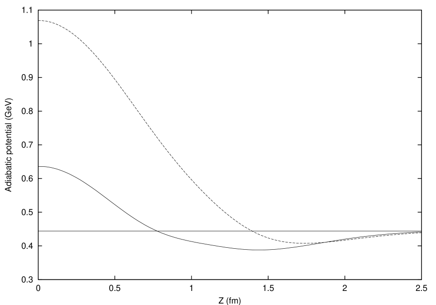
FIG. 12.: The adiabatic potential in the molecular orbital basis for $\displaystyle SI$ = (10) (full curve) and $\displaystyle SI$ = (01) (dashed curve) with pseudoscalar + scalar quark-quark interaction.

REFERENCES

- [1] M. Oka and K. Yazaki, Int.Rev.Nucl.Phys., vol. 1 (Quarks and Nuclei, ed. W. Weise), World Scientific, Singapore, p. 490 (1984)
- [2] K. Shimizu, Rep.Prog.Phys. 52 (1989) 1
- [3] A. M. Kusainov, V. G. Neudatchin and I. T. Obukhovsky, Phys.Rev. C44 (1991) 1343
- [4] Z. Zhang, A. Faessler, U. Straub and L.Ya. Glozman, Nucl.Phys. A578 (1994) 573; A. Valcarce, A. Buchman, F. Fernandez and A. Faessler, Phys.Rev. C50 (1994) 2246
- [5] Y. Fujiwara, C. Nakamoto and Y. Suzuki, Phys..Rev.Lett. 76 (1996) 2242; Phys.Rev. C54 (1996) 2180
- [6] D. Bartz and Fl. Stancu, Phys.Rev. C59 (1999) 1756
- [7] L. Ya. Glozman and D. O. Riska, Phys. Rep. 268 (1996) 263
- [8] L. Ya. Glozman, Z. Papp and W. Plessas, Phys. Lett. B381 (1996) 311
- [9] L. Ya. Glozman, Z. Papp, W. Plessas, K. Varga and R.F. Wagenbrunn, Nucl.Phys. A623 (1997) 90c
- [10] H. Collins and H. Georgi, Phys. Rev. D59 (1999) 094010
- [11] L. Ya. Glozman and K. Varga, e-print hep-ph/9901439
- [12] M. C. Chu et al., Phys. Rev. D49 (1994) 6039; J. W. Negele, e-print hep-lat/9810053; K. F. Liu et al., LANL e-print hep-ph/9806491
- [13] Fl. Stancu, S. Pepin and L.Ya. Glozman, Phys.Rev. C56 (1997) 2779
- [14] M. Harvey, Nucl. Phys. A352 (1981) 301; ibid. A481 (1988) 834
- [15] Fl. Stancu and L. Wilets, Phys.Rev. C36 (1987) 726
- [16] W. Koepf, L. Wilets, S. Pepin and Fl. Stancu, Phys. Rev. C50 (1994) 614
- [17] D. Robson, Phys. Rev. D35 (1987) 1029
- [18] G. E. Brown and A. D. Jackson, The nucleon-nucleon interaction, North Holland, Amsterdam, 1976 p. 5
- [19] T. Schäfer and E. V. Shuryak, Rev. Mod. Phys. 70 (1998) 323
- [20] D. O. Riska and G. E. Brown, e-print hep-ph/9902319
- [21] L. Ya. Glozman, W. Plessas, K. Varga and R. Wagenbrunn, Phys. Rev. D58 (1998) 094030
- [22] Fl. Stancu, Group Theory in Subnuclear Physics, Clarendon Press, Oxford, 1996, chapters 4 and 10
- [23] S. Wolfram, The Mathematica book, Wolfram Media/Cambridge University Press, Cambridge, 1996
- [24] Ch. Elster and K. Holinde, Phys. Lett. 136B (1984) 135; K. Holinde, Nucl. Phys. A415 (1984) 427
- [25] K. Shimizu, private communication