DTP/99/20

March 1999

Saturation in Diffractive Deep Inelastic Scattering

K.  Golec-Biernat^2,1 and M. Wüsthoff¹

¹Department of Physics, University of Durham, Durham DH1 3LE, UK

²H. Niewodniczanski Institute of Nuclear Physics, Department of Theoretical Physics, Radzikowskiego 152, Krakow, Poland

We successfully describe the HERA-data on diffractive deep inelastic scattering using a saturation model which has been applied in our earlier analysis of the inclusive $ep$-scattering data. No further parameters are needed. Saturation already turned out to be essential in describing the transition from large to small values of $Q^{2}$ in inclusive scattering. It is even more important for diffractive processes and naturally leads to a constant ratio of the diffractive versus inclusive cross sections. We present an extensive discussion of our results as well as detailed comparison with data.

1 Introduction

In a recent analysis [1] we introduced a model which provides a description of the transition between large and low $Q^{2}$ in inclusive lepton–proton deep inelastic scattering at low $x$. The idea behind our model is a phenomenon which we call a combined saturation at low $Q^{2}$ and low $x$. In this kinematical region the size of the virtual probe is of the order of the mean transverse distance between partons in the proton. The cross section for the interaction between the probe and the partons becomes large and multiple scattering has to be taken into account. These effects lead to saturation of the total cross section. We found that saturation occurs at low but still perturbative values of $Q^{2}$ ($\sim 1-2~{}GeV^{2}$ for $x=10^{-4}$). We therefore believe that saturation should be described by means of perturbative QCD (see also for example Ref. [2, 3, 4, 5]).

The QCD-framework we use allows us to describe not only inclusive but diffractive processes as well. A general feature of diffraction is its strong sensitivity towards the infrared regime even for large $Q^{2}$. The fact that diffraction has a strong soft component has already been noticed earlier, leading to the assumption that the Pomeron in diffraction ought to be soft. The idea of saturation, however, emphasizes the transition from hard to soft physics. As mentioned earlier saturation effects become already viable at rather hard scales and strongly suppress soft contributions in diffractive processes [6]. This mechanism leads to an effective enhancement of hard contributions and hence to an effective Pomeron intercept which lies above the original soft value.

The important conclusion of this paper is that the concept of saturation leads to a good description of the diffractive data. Our approach has the important property that the inclusive and diffractive cross section have the same power-behavior in $x$. We have obtained these results without the use of any additional fitting parameters, i.e. we solely take the model as determined in Ref. [1] from the analysis of inclusive processes. The diffractive slope which we use is taken from the measurement at HERA.

The plan of our paper is as follows. In Section 2 and 3 we recapitulate the results found in Ref. [1] and discuss qualitatively the basic features of saturation for both inclusive and diffractive processes. In Section 4 we provide the detailed formulae for our numerical analysis and discuss the comparison with the data from H1 [7] and ZEUS [8] in Section 5. In Section 6 we present the impact parameter version of our results and finish with concluding remarks in Section 7. The Appendix was added to enclose some details on the derivation of the cross section formulae for diffractive scattering. In particular it contains the computation of the relevant set of Feynman diagrams which contribute to the quark-antiquark-gluon final state.

2 Saturation in inclusive processes

Our starting point in Ref. [1] was the well established physical picture of small-$x$ interactions in which the photon with virtuality $Q^{2}$, emitted by a lepton, dissociates into a quark-antiquark pair far upstream of the nucleon (in the nucleon rest frame). The dissociation is then followed by the scattering of the quark-antiquark pair on the nucleon. In this picture the relative transverse separation ${\bf r}$ of the $q\bar{q}$ pair and the longitudinal photon momentum fraction $\alpha$ of the quark ($1-\alpha$ for the antiquark) are good degrees of freedom. In these variables the $\gamma^{*}p$ cross sections have the following factorized form [9, 10]

$$\sigma_{T,L}(x,Q^{2})\>=\>\int\!d\,^{2}{\bf r}\!\int_{0}^{1}\!d\alpha\>|\Psi_{T,L}\,(\alpha,{\bf r})|^{2}\>\hat{\sigma}\,(x,r^{2})\;,\\$$ (1)

where $\Psi_{T,L}$ is the squared photon wave function for the transverse $(T)$ and longitudinally polarized $(L)$ photons, given by

$$|\Psi_{T,L}\,(\alpha,{\bf r})|^{2}\,=\,\frac{6\,\alpha_{em}}{4\,\pi^{2}}\,\sum_{f}\,e_{f}^{2}\,\cases{[\,\alpha^{2}+(1-\alpha)^{2}\,]\>\overline{Q}^{2}\,K_{1}^{2}\,(\overline{Q}\,r)\,+\,m_{f}^{2}\>K_{0}^{2}\,(\overline{Q}\,r)\,\cr\cr 4\,Q^{2}\,\alpha^{2}\,(1-\alpha)^{2}\,K_{0}^{2}\,(\overline{Q}\,r)\;.}$$ (2)

In the above formulae $K_{0}$ and $K_{1}$ are Mc Donald-Bessel functions and

$$\overline{Q}^{2}\>=\>\alpha\,(1-\alpha)\,Q^{2}\,+\,m_{f}^{2}\;.$$ (3)

The dynamics of saturation is embedded in the the effective dipole cross section $\hat{\sigma}(x,r)$ which describes the interaction of the $q\bar{q}$ pair with a nucleon:

$$\hat{\sigma}(x,r^{2})\,=\,\sigma_{0}\,\left\{1\,-\,\exp\left(-\frac{r^{2}}{4R_{0}^{2}(x)}\right)\right\}\;,$$ (4)

where the $x$-dependent radius $R_{0}$ is given by

$$R_{0}(x) = \frac{1}{GeV}\;\left(\frac{x}{x_{0}}\right)^{\lambda/2}\;.$$ (5)

The normalization $\sigma_{0}$ and the parameters $x_{0}$ and $\lambda>0$ of $R_{0}(x)$ have been determined by a fit to all inclusive data on $F_{2}$ with $x<0.01$  [1]. (the detailed values of these parameters are quoted in Section 5).

Figure 1: The integrand of the inclusive cross section $\sigma_{T}$ in (1) (solid lines) after the integration over $\alpha$ and the azimuthal angle, plotted for two values of $Q^{2}$. The dotted lines show the dipole cross section (4). The dashed vertical lines correspond to the characteristic scales $r=2R_{0}$ and $r=2/Q$. The values for $2R_{0}$ at a fixed energy $W=245~{}\mbox{\rm GeV}$ are: $0.36~{}\mbox{\rm fm}$ for $Q^{2}=10~{}\mbox{\rm GeV}^{2}$ and $0.25~{}\mbox{\rm fm}$ for $Q^{2}=0.8~{}\mbox{\rm GeV}^{2}$.

Saturation in the dipole cross section (4) sets in when $r\sim 2R_{0}$, allowing a good description of the data at low $Q^{2}$ when $1/Q>R_{0}$ (see right plot in Fig. 1). The detailed analysis of Eqs. (1)-(4), presented in Ref. [1], gives for small $Q^{2}$

$$\sigma_{T}\,\sim\,\sigma_{0}\,.$$ (6)

For large $Q^{2}$ the dominant contribution comes from small dipole configurations with $r\sim 2/Q\ll R_{0}$ (see left plot in Fig. 1). In this case we have the usual situation of color transparency, $\hat{\sigma}\sim r^{2}$, which gives the scaling behavior of the $\gamma^{*}p$ cross sections

$$\sigma_{T}\sim{1}/{Q^{2}}\,.$$ (7)

More precise analysis leads to logarithmic in $Q^{2}$ modifications of the above estimations. To summarize, the saturation model naturally interpolates between the two different regimes of $\sigma_{T}$ described by Eqs. (6) and (7).

Saturation is characterized by a ‘critical line’ in the $(x,Q^{2})$-plane given by the equation $Q^{2}=1/R_{0}^{2}(x)$ [1, 2, 4]. It is important to note that at very small $x$ saturation effects become relevant at fairly high scales ($Q^{2}\sim 1-2~{}GeV^{2}$ for HERA energies [1]) where one believes that perturbative QCD is valid. The critical line divides the phase space into two regions, the scaling region in which relation (7) is valid and the saturation region with the behavior given by Eq. (6).

The physical picture behind saturation is based on interpretation of the $x$-dependent radius $R_{0}(x)$ as the mean separation of partons in the proton. We see from (5) that when $x$ decreases so does the mean seperation. Thus at low $x$ the distribution of partons in the proton is no longer dilute when probed by a virtual photon of fixed resolution ($\sim 1/Q$) and saturation sets in. This happens when the resolution of the probe equals to the mean separation, $1/Q=R_{0}(x)$, which condition defines the ”critical line”. As a result the dipol cross section becomes large and mulitple interactions become important. In other words, at low $x$ proton appears to be black. The important result of our inclusive analysis is that blackening occurs already at rather short distances well below where ’soft dynamics’ is supposed to set in, justifying the use of perturbative QCD.

In the scaling region of large $Q^{2}$ the growth of the inclusive cross section is driven by the increase in the number of partons since the gluon density $G(x)$ is proportional to $1/R_{0}^{2}(x)$ (see Section 4 for detailes of this relation). This grows is eventually tamed in our model by the mechanism of saturation.

3 Saturation in diffractive deep inelastic scattering

Inclusive $\gamma^{*}p$ cross section at large $Q^{2}$ is dominated by the scaling region. Diffractive scattering on the other hand is essentially determined by the saturation region. In this case the dependence on $x$ is controlled by the available phase space in the transverse momentum. This phase space grows proportional to $1/R_{0}^{2}(x)$ and leads to the same power behavior in $x$ as was found for the inclusive cross section. It also means that the average transverse momentum of the diffractive final state will increase when $x$ decreases. The process becomes ’harder’ when $x$ becomes smaller. Crucial for this picture to work is the scale invariance which in our approach is maintained by the lack of any additional cutoff on the transverse momenta of the final state. We will discuss this conclusion in more details below.

In order to demonstrate the main features of saturation in diffraction we will confine our discussion in this section to the elastic scattering of the $q\bar{q}$-pair as shown in Fig. 3a. Elastic $q\bar{q}$-scattering dominates diffractive $\gamma^{*}p$ scattering for not to large values of the diffractive mass $M$. At large $M$, however, the emission of a gluon as depicted in Fig. 3b becomes the dominant contribution. The cross section for elastic $q\bar{q}$-scattering takes on the following form

$$\left.\frac{d\sigma_{T,L}^{D}}{dt}\right|_{t=0}\;=\;\frac{1}{16\pi}\;\int\!d\,^{2}{\bf r}\!\int_{0}^{1}\!d\alpha\>|\Psi_{T,L}\,(\alpha,{\bf r})|^{2}\>\hat{\sigma}^{2}\,(x,r^{2})\;.\\$$ (8)

with the same dipole cross section $\hat{\sigma}$ as introduced for inclusive scattering. We account for the $t-$dependence by assuming an exponential dependence with the diffractive slope $B_{D}$. Thus the $t$-integrated diffractive cross section equals

$$\sigma^{D}(x,Q^{2})\;=\;\int_{-\infty}^{0}dt\,e^{B_{D}t}\,\left.\frac{d\sigma^{D}}{dt}\right|_{t=0}\;=\;\frac{1}{B_{D}}\,\left.\frac{d\sigma^{D}}{dt}\right|_{t=0}\,,$$ (9)

for both longitudinal and transverse photons.

Figure 2: The integrands of the inclusive (Inc) and diffractive (DD) cross sections at $Q^{2}=10~{}GeV^{2}$ for the following two cases: (a) saturation according to Eq. (4) (dotted line) and (b) no saturation, i.e. $\hat{\sigma}\sim r^{2}$ .

The distributions in $r$ ($q\bar{q}$ dipole size) of the integrand for inclusive (Eq. (1)) and diffractive (Eq. (8)) scattering at $Q^{2}=10~{}GeV^{2}$ are shown in Fig. 2. The integrations over $\alpha$ and the azimuthal angle have been performed. The dotted lines denote the dipole cross section $\hat{\sigma}$. Comparing the two solid lines in Fig. 2a we see that for a typical inclusive event the main contribution is located around $r\sim 2/Q\ll 2R_{0}$. The diffractive cross section on the other hand is dominated by the saturation region $r\sim 2R_{0}$. The importance of saturation for diffraction is illustrated in Fig. 2b where we let $\hat{\sigma}$ rise proportionally to $r^{2}$. While this change has only little effect on the inclusive cross section, the diffractive cross section becomes strongly divergent One, in fact, needs an infrared cutoff - a new, additional scale $R_{cut}$ - to be introduce by hand. As a consequence an additional factor $R_{cut}^{2}/R_{0}^{2}(x)$ emerges which leads a result reminiscent of the triple Regge approach where $\sigma^{D}\sim x^{-2\lambda}$ instead of $\sigma^{D}\sim x^{-\lambda}$ as we find with saturation.

Fig. 2 also illustrates the idea of Ref. [6] that diffraction at small $x$ is not a purely soft but semi-hard process. Let us assume for simplicity that the ’soft regime’ begins at $r=4R_{0}$. It becomes quite clear by comparing the two plots in Fig. 2 how strongly the soft contribution is suppressed due to saturation (blackness of the nucleon). The relative fraction of hard contributions ($r<2R_{0}$) is enhanced to almost 50%, making diffractive deep inelastic scattering a semi-hard process. A related issue is the smallness of the profile function in central collisions in $p\bar{p}$ scattering and its consequence for single diffraction.

The following qualitative estimates will help to clarify the remarks about the importance of saturation for diffraction. The wave function in Eq. (2) can be approximated by (see also Ref. [11, 10])

$$|\Psi_{T,L}\,(\alpha,{\bf r})|^{2} \approx \frac{6\,\alpha_{em}}{4\,\pi^{2}}\,\sum_{f}\,e_{f}^{2}\,\cases{[}\,\alpha^{2}+(1-\alpha)^{2}\,]\;\frac{1}{r^{2}}\;\Theta[\alpha(1-\alpha)Q^{2}r^{2}<1]\;\;.$$ (10)

The leading contribution is associated with the ’aligned jet’ configuration. In the $\gamma^{*}$-Pomeron CMS the scattering angle $\theta$ is given by $\cos(\theta)=1-2\alpha$, i.e. for $\alpha\rightarrow 0\;(1)$ we have $\theta\rightarrow 0\;(\pi)$. The $\Theta$-function in Eq. (10) enforces the condition that either $\alpha$ or $1-\alpha$ is smaller than $1/(Q^{2}r^{2})$. We make use of this condition and the $\alpha\leftrightarrow 1-\alpha$ symmetry to perform the $\alpha$-integration in Eqs. (1) and (9) and obtain

$$\sigma(x,Q^{2}) \approx \frac{6\,\alpha_{em}}{2\,\pi}\,\sum_{f}\,e_{f}^{2}\;\frac{1}{Q^{2}}\;\int_{4/Q^{2}}^{\infty}\!\frac{d\,r^{2}}{r^{4}}\;\hat{\sigma}\,(x,r^{2})$$

$$\sigma^{D}(x,Q^{2}) \approx \frac{6\,\alpha_{em}}{32\,\pi^{2}\,B_{D}}\,\sum_{f}\,e_{f}^{2}\;\frac{1}{Q^{2}}\int_{4/Q^{2}}^{\infty}\!\frac{d\,r^{2}}{r^{4}}\;\hat{\sigma}^{2}\,(x,r^{2})\;\;.$$

The lower limit is required, since the factor $1/(Q^{2}r^{2})$ which results from the $\alpha$-integration should not exceed 1/4. We also approximate the dipole cross section (4) by

$$\hat{\sigma} \approx \cases{\sigma_{0}\;r^{2}/[4R_{0}^{2}(x)]&for \hskip 14.22636pt$r^{2}<4R_{0}^{2}(x)$\cr\cr\sigma_{0}&for \hskip 14.22636pt$r^{2}>4R_{0}^{2}(x)$}\,$$ (12)

Inserting (12) into (3) gives after integration

$$\sigma(x,Q^{2}) \approx \frac{6\,\alpha_{em}}{2\,\pi}\,\sum_{f}\,e_{f}^{2}\;\frac{\sigma_{0}}{4R_{0}^{2}(x)\;Q^{2}}\;\ln[R_{0}^{2}(x)\;Q^{2}]$$

$$\sigma^{D}(x,Q^{2}) \approx \frac{6\,\alpha_{em}}{16\,\pi^{2}\,B_{D}}\,\sum_{f}\,e_{f}^{2}\;\frac{\sigma_{0}^{2}}{4R_{0}^{2}(x)\;Q^{2}}\;\;.$$

Thus we obtain an approximate constant ratio of the diffractve to inclusive cross sections similar to the exact result in Ref. [1]

$$\frac{\sigma^{D}}{\sigma} \approx \frac{\sigma_{0}}{8\,\pi\,B_{D}}\;\frac{1}{\ln[R_{0}^{2}(x)\;Q^{2}]}\;\;.$$ (14)

If, on the other hand, we had used

$$\hat{\sigma}(x,Q^{2}) \approx \sigma_{0}\;\frac{r^{2}}{4R_{0}^{2}(x)}$$ (15)

instead of (3), i.e. no saturation, then a cutoff $R_{cut}^{2}$ would be required leading to

$$\sigma(x,Q^{2}) \approx \frac{6\,\alpha_{em}}{2\,\pi}\,\sum_{f}\,e_{f}^{2}\;\frac{\sigma_{0}}{4R_{0}^{2}(x)\,Q^{2}}\;\ln(R_{cut}^{2}\;Q^{2}/4)$$

$$\sigma^{D}(x,Q^{2}) \approx \frac{6\,\alpha_{em}}{32\,\pi^{2}\,B_{D}}\,\sum_{f}\,e_{f}^{2}\;\frac{\sigma_{0}^{2}\;R_{cut}^{2}}{[4R_{0}^{2}(x)]^{2}\,Q^{2}}\;\;.$$

The important point is that the inclusive cross section depends only weakly on $R_{cut}$ whereas the diffractive cross section shows a strong dependence. We also realize that under the assumption (15) the diffractive cross section, being proportional to $1/R^{4}_{0}(x)$, rises at small $x$ twice as strongly as the inclusive cross section ($\sim x^{-2\lambda}$ as mentioned earlier). The ratio (14) would be proportional to $x^{-\lambda}$ which is clearly not observed at HERA.

To summarize, since the diffractive cross section is so sensitive to the infrared cutoff which is effectively given by $2R_{0}(x)$ one can conclude that diffraction directly probes the transition region. We will now turn to a full description of the diffractive deep inelastic scattering data from HERA.

4 Diffractive structure function in momentum space representation

In this section we summarize the relevant contributions to the diffractive structure function. We use the standard notation for the variables $\beta=Q^{2}/(M^{2}+Q^{2})$ and $x_{I\!\!P}=(M^{2}+Q^{2})/(W^{2}+Q^{2})$ where $M$ is the diffractive mass and $W$ the total energy of the $\gamma^{*}p$-process.

Before we start to compute the diffractive structure function it is useful to introduce the unintegrated gluon distribution ${\cal F}$ which is related to the effective dipole cross section $(\ref{sigmahat})$ in the following way [9, 10]:

$$\hat{\sigma}(x,r) = \frac{4\pi}{3}\;\int\frac{d^{2}{\bf l}_{t}}{l_{t}^{2}}\;\left[\;1-e^{i\;{\bf r}\cdot{\bf l}}\;\right]\;\alpha_{s}\,{\cal F}(x,l_{t}^{2})$$

$$= \frac{4\pi^{2}}{3}\;\int\frac{dl^{2}_{t}}{l_{t}^{2}}\;\left[\;1-J_{0}(l_{t}r)\;\right]\;\alpha_{s}\,{\cal F}(x,l_{t}^{2})\;\;.$$

A short calculation shows that with the following form for $\cal{F}$

$$\alpha_{s}\,{\cal F}(x,l_{t}^{2})=\frac{3\;\sigma_{0}}{4\pi^{2}}\;R_{0}^{2}(x)\;l_{t}^{2}\;e^{-R_{0}^{2}(x)l_{t}^{2}}\;\;,$$ (18)

one can indeed reproduce Eq. (4). At large $Q^{2}$ the usual gluon distribution $G$ can be calculated from ${\cal F}$ by a simple integration:

$$x\,G(x,Q^{2}) = \int_{0}^{Q^{2}}dl_{t}^{2}\;{\cal F}(x,l_{t}^{2})$$

$$= \frac{3}{4\pi^{2}\alpha_{s}}\;\frac{\sigma_{0}}{R_{0}^{2}(x)}\;\left[1-(1+Q^{2}R_{0}^{2})\;e^{-Q^{2}R_{0}^{2}}\right]$$

$$\simeq \frac{3}{4\pi^{2}\alpha_{s}}\;\frac{\sigma_{0}}{R_{0}^{2}(x)},\;\;\;\;\;\;(Q^{2}R^{2}_{0}(x)\gg 1)$$

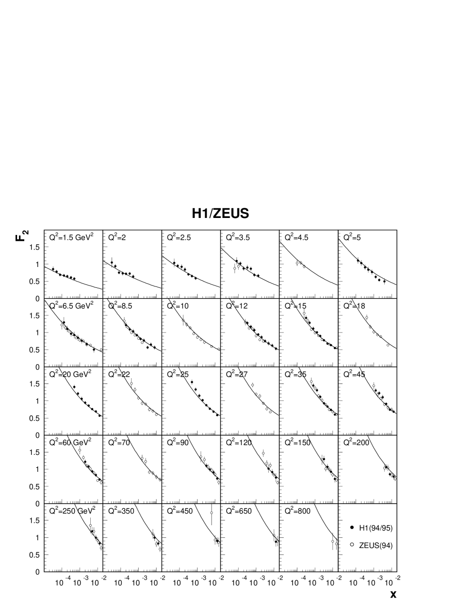
Figure 6: The results (solid lines) of the fit to the inclusive HERA data on $F_{2}$ for different values of $Q^{2}$, using the model of $[1]$ with saturation.

Important to note is the fact that at large $Q^{2}$ the gluon distribution exhibits a plain scaling behavior. The proper DGLAP evolution in $Q^{2}$ for the gluon can be added to our model, e.g. by treating relation (4) as the initial distribution for the linear DGLAP evolution equations. However the results of our model presented in Fig. 6 suggest that the $Q^{2}$ dependence of the data at low $x$ values are properly accounted for in the presented approach and the additional gluonic evolution will only lead to a moderate improvement.

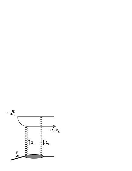
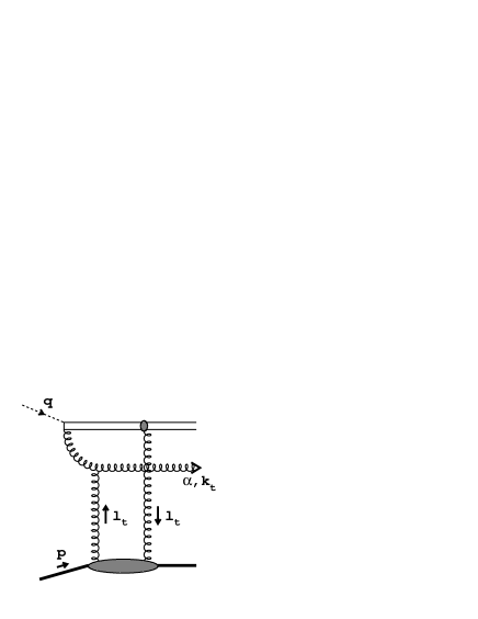
Figure 3: Diffractive production of a $q\bar{q}$-pair (left) and the emission of an additional gluon (right).

We have three terms owing to the diffractive production of a quark-antiquark pair with transverse and longitudinally polarized photons and the emission of an extra gluon in the final state (Fig. 3). The latter contribution is only known at present in certain approximations: strong ordering in the transverse momenta or strong ordering in the longitudinal momentum components. The first approximation is valid at a very large $Q^{2}$ and finite diffractive masses, i.e. finite $\beta$, and picks out the leading logarithm in $Q^{2}$ from the quark box. The second approximation is valid for large diffractive masses, i.e. small $\beta$, and finite $Q^{2}$ [12]. Since the diffractive data range around $\beta=0.5$ we will pursue the first approximation and assume that the transverse momenta of the quarks compared to the gluon are much larger.

For a detailed discussion of the derivation of the following formulae we refer to Ref. [13] and only quote the result:

$$x_{I\!\!P}F_{\{t,q\bar{q}\}}^{D}(Q^{2},\beta,x_{I\!\!P}) = \frac{1}{96B_{D}}\;\sum_{f}e^{2}_{f}\;\frac{Q^{2}}{1-\beta}\;\int_{0}^{1}d\alpha\;[\alpha^{2}+(1-\alpha)^{2}]\;$$

$$\times \left\{\int\frac{dl_{t}^{2}}{l_{t}^{2}}\alpha_{s}{\cal F}(x_{I\!\!P},l_{t}^{2})\left[1-2\beta\;+\;\frac{l_{t}^{2}-(1-2\beta)\;k^{2}}{\sqrt{[l_{t}^{2}+k^{2}]^{2}-4(1-\beta)\;l_{t}^{2}\;k^{2}}}\right]\right\}^{2}$$

and

$$x_{I\!\!P}F_{\{l,q\bar{q}\}}^{D}(Q^{2},\beta,x_{I\!\!P}) = \frac{1}{6B_{D}}\;\sum_{f}e^{2}_{f}\;\int_{0}^{1}d\alpha\;k^{2}\;\beta^{2}\;\;$$

$$\times \left\{\int\frac{dl_{t}^{2}}{l_{t}^{2}}\alpha_{s}{\cal F}(x_{I\!\!P},l_{t}^{2})\left[1\;-\;\frac{k^{2}}{\sqrt{[l_{t}^{2}+k^{2}]^{2}-4(1-\beta)\;l_{t}^{2}\;k^{2}}}\right]\right\}^{2}\;\;.$$

We have introduced the variable $k^{2}$ which is defined as

$$k^{2} = \alpha(1-\alpha)\frac{Q^{2}}{\beta}=\frac{k_{t}^{2}}{1-\beta}$$ (22)

and describes the mean virtuality of the exchange quark in the upper part of the diagram. Eq. (22) follows from the kinematics of the two-body final state. The variable $\alpha$ stems from the Sudakov decomposition: $k=\alpha q^{\prime}+({|k_{t}^{2}|/}{2\alpha q^{\prime}\cdot p})p+k_{t}$ and $q^{\prime}=q+xp$. The unintegrated structure function ${\cal F}$ is visualized in Fig. 3 as the lower blob. It is related to the inclusive $F_{2}$ by the optical theorem for zero momentum transfer $t$. In order to include the $t$-averaged distribution we have simply divided all expressions by the diffractive slope parameter $B_{D}$ which has to be taken from the measurement, see Eq. (9).

The third contribution takes on the form:

$$x_{I\!\!P}F_{\{t,q\bar{q}g\}}^{D}(Q^{2},\beta,x_{I\!\!P}) = \frac{9\;\beta}{64B_{D}}\,\sum_{f}e_{f}^{2}\;\int_{0}^{Q^{2}}dk^{2}\;\frac{\alpha_{s}}{2\pi}\;\ln\left(\frac{Q^{2}}{k^{2}}\right)\;\;\int_{\beta}^{1}\frac{dz}{z^{2}\,(1-z)^{2}}\;$$

$$\times \left[\left(1-\frac{\beta}{z}\right)^{2}+\left(\frac{\beta}{z}\right)^{2}\right]\left\{\int\frac{dl_{t}^{2}}{l_{t}^{2}}\;\alpha_{s}{\cal F}(x_{I\!\!P},l_{t}^{2})\;\;\right.$$

$$\times \left.\left[z^{2}+(1-z)^{2}+\frac{l_{t}^{2}}{k^{2}}-\frac{[(1-2z)k^{2}-l_{t}^{2}]^{2}+2z(1-z)k^{4}}{k^{2}\sqrt{(l_{t}^{2}+k^{2})^{2}-4(1-z)\;l_{t}^{2}\;k^{2}}}\right]\right\}^{2}\;\;.$$

In analogy to the previous formulae the variable $k^{2}$ expresses the mean virtuality of the exchanged gluon in the upper part of the right diagram (Fig. 3):

$$k^{2} = \frac{k_{t}^{2}}{1-z}\;\;.$$ (24)

The variable $z$ represents the momentum fraction of the upper $t$-channel gluon with respect to the Pomeron momentum $x_{I\!\!P}p$. It needs to be stressed that this formula was derived in the spirit of a leading log($Q^{2}$) approximation which introduces uncertainties besides those related to the choice of $\alpha_{s}$. In this approximation the true kinematical constraints are not exactly fulfilled. The violation of these constraints, however, gives contributions which are sub-leading in the limit of very large $Q^{2}$. An improvement can be achieved by an exact Monte Carlo integration. The exact treatment of the phase space, however, has to go along with the use of the exact matrix-element which is not known up to now. Similar analytic results can be found in Ref. [14]. The main difference as compared to our approach is hidden in the unintegrated gluon distribution which in Ref. [14] is modeled by a heavy quark-antiquark pair.

There are two limits which are interesting to look at and which have been discussed in the literature: the first limit is the triple Regge limit (small $\beta$) in which $z$ can be set to zero in the square bracket of Eq. (4). This leads to

$$x_{I\!\!P}F_{\{t,q\bar{q}g\}}^{D}(Q^{2},\beta,x_{I\!\!P}) = \frac{9\;\beta}{64B_{D}}\,\sum_{f}e_{f}^{2}\;\int_{0}^{Q^{2}}dk^{2}\;\frac{\alpha_{s}}{2\pi}\;\ln\left(\frac{Q^{2}}{k^{2}}\right)\;\;\int_{\beta}^{1}\frac{dz}{z^{2}}\;$$

$$\times \left[\left(1-\frac{\beta}{z}\right)^{2}+\left(\frac{\beta}{z}\right)^{2}\right]\left\{\int\frac{dl_{t}^{2}}{l_{t}^{2}}\;\alpha_{s}{\cal F}(x_{I\!\!P},l_{t}^{2})\;\;\right.$$

$$\times \left.2\;\left[\Theta(l_{t}^{2}-k^{2})+\frac{l_{t}^{2}}{k^{2}}\Theta(k^{2}-l_{t}^{2})\right]\right\}^{2}\;\;$$

and agrees with results of Refs. [12, 15, 16]. The other limit is $l_{t}^{2}\ll k^{2}$ and requires a lower cutoff $k_{0}^{2}$ on $k^{2}$:

$$x_{I\!\!P}F_{\{t,q\bar{q}g\}}^{D}(Q^{2},\beta,x_{I\!\!P}) = \frac{9\;\beta}{64B_{D}}\,\sum_{f}e_{f}^{2}\;\int_{k_{0}^{2}}^{Q^{2}}dk^{2}\;\frac{\alpha_{s}}{2\pi}\;\ln\left(\frac{Q^{2}}{k^{2}}\right)\;\;\int_{\beta}^{1}\frac{dz}{z^{2}\,(1-z)^{2}}\;$$

$$\times \left[\left(1-\frac{\beta}{z}\right)^{2}+\left(\frac{\beta}{z}\right)^{2}\right]\left\{\;\alpha_{s}x_{I\!\!P}G(x_{I\!\!P},k^{2})\;\;\right.$$

$$\times \left.2\;(1-z)^{2}\;(1+2z)\;\frac{1}{k^{2}}\;\right\}^{2}\;\;.$$

This result and corresponding approximations for Eqs. (4) and (4) have been derived earlier in Ref. [17]. They have been utilized in Ref. [18] to perform a similar analysis of diffraction as presented in this paper. The approximations used in Ref. [18] allow the direct implementation of the gluon structure function as given by standard parameterizations. The result is a too steep increase of the diffractive structure function with decreasing $x_{I\!\!P}$. The exact formulae in conjunction with saturation give a much shallower behaviour which is in better agreement with the data (see below).

5 Comparison with data

Before we start our numerical investigation into diffractive scattering we would like to review the fit to the inclusive data [1]. The expression for the structure function $F_{2}$ we have used in [1] was derived from Eq. (1) in combination with the saturation model (4) quoted in Section 2. The parameters were found to be $\sigma_{0}=23.03~{}\mbox{\rm mb}$, $\lambda=0.288$ and $x_{0}=3.04\cdot 10^{-4}$. These parameters enter into the diffractive cross section via the function ${\cal F}$ in Eqs. (4-4). To illustrate the quality of the fit we plot in Fig. 6 the structure function $F_{2}(x,Q^{2})$ in different $Q^{2}$ bins in comparison with the data from H1 [19] and ZEUS [20] (see also [1] for different comparison).

The remaining integrations in Eqs. (4-4) have been performed numerically. We consider three light flavors and assume the diffractive slope parameter $B_{D}=6~{}GeV^{-2}$ which is somewhat lower than the reported value of $7.1~{}GeV^{-2}$ [21]. One has, however, to take into account some corrections due to double dissociation (dissociation of the proton) which can be roughly estimated by lowering the diffractive slope from 7.1 to 6 $GeV^{-2}$. The coupling constant is kept fixed: $\alpha_{s}=0.2$.

Fig. 7 shows our result for the diffractive structure function $x_{{I\!\!P}}F^{D}(x_{{I\!\!P}},\beta,Q^{2})$ at fixed $x_{{I\!\!P}}=0.0042$ plotted over $\beta$ for various $Q^{2}$ together with data from ZEUS [8]. Fig. 8 contains similar plots with H1-data for fixed $x_{{I\!\!P}}=0.003$ [7]. The three contributions (4), (4) and (4) have been displayed separately in Fig. 7. The important feature is the separation in three distinct regimes of small, medium and high $\beta$ where the production of $q\bar{q}g$, $q\bar{q}$ with transverse and $q\bar{q}$ with longitudinally polarized photons, respectively, is dominant. It was already argued in Ref. [22] that this behavior is mainly due to the nature of the wave functions rather than the model we use. The relative strength of the three contributions is fixed by QCD-color factors. The overall normalization, however, directly results from the saturation model without any fits to diffractive data. This fact is important to point out, since in Ref. [22] the overall and the relative normalization for the mentioned three contributions was fitted. One should note that there is no hard gluon component present in our approach (compare the analyses based on the concept of the ‘soft’ Pomeron structure function [7, 28]).

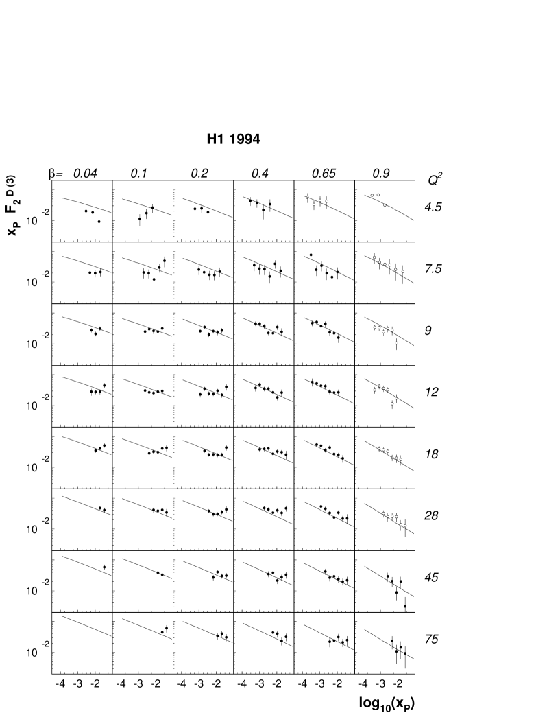
Figure 10: The same as in Fig. 9 but for H1 data. $Q^{2}$ values are in units of $GeV^{2}$.

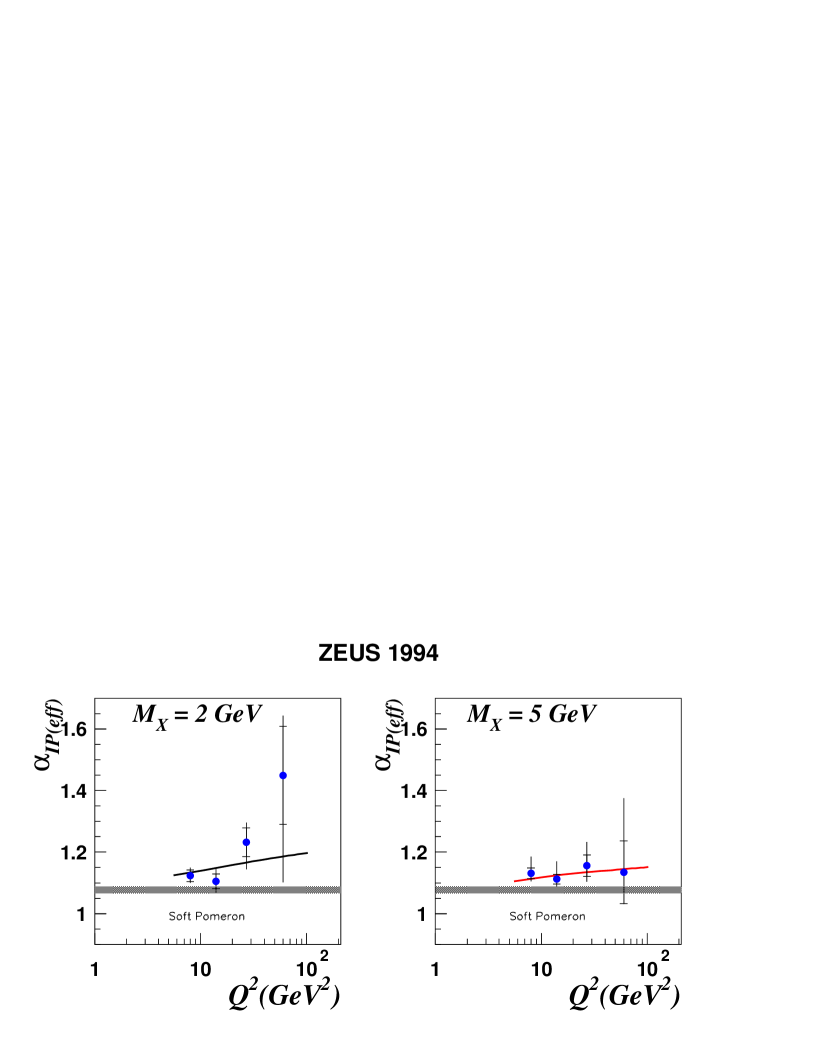
Figure 11: The effective Pomeron slope as defined in the text as a function of $Q^{2}$ for two values of the diffractive mass $M$.

The prediction of the $x_{I\!\!P}$-dependence, besides the overall normalization, is an important consequence of the saturation model. In Fig. 9 and Fig. 10 we compare our predictions with the data for $x_{{I\!\!P}}F^{D}(x_{{I\!\!P}},\beta,Q^{2})$, now analyzed as a function of $x_{{I\!\!P}}$ for different values of $\beta$ and $Q^{2}$. Notice the good agreement, especially in the region of moderate and large values of $\beta$ which corresponds to not too large values of the diffractive mass $M$. We also reproduce the change of the effective Pomeron intercept $\bar{\alpha}_{{I\!\!P}(eff)}$ as a function of $Q^{2}$ for different diffractive masses $M$, see Fig. 11. The effective intercept is related to the logarithmic $x_{{I\!\!P}}$-slope $n$ of $x_{{I\!\!P}}F^{D}(x_{{I\!\!P}},\beta,Q^{2})$ through the relation: $n=1-2\bar{\alpha}_{{I\!\!P}(eff)}$. At low masses $M$ where the longitudinal part dominates the slope in $x_{I\!\!P}$ is slightly steeper due to the enhanced longitudinal part of the cross section. Using the effective Pomeron intercept means having incorporated shrinkage in the context of soft Regge phenomenology. The rise in $Q^{2}$ is again mainly caused by the longitudinal part. There is, however, another effect at work which lowers the intercept at small $\beta$. The $q\bar{q}g$-contribution has a logarithm $\ln(Q^{2}/k^{2})$ which is approximately equal to $\ln(Q^{2}R_{0}(x)^{2})$. This term effectively lowers the intercept in the regime where $q\bar{q}g$ dominates, i.e. at small $\beta$.

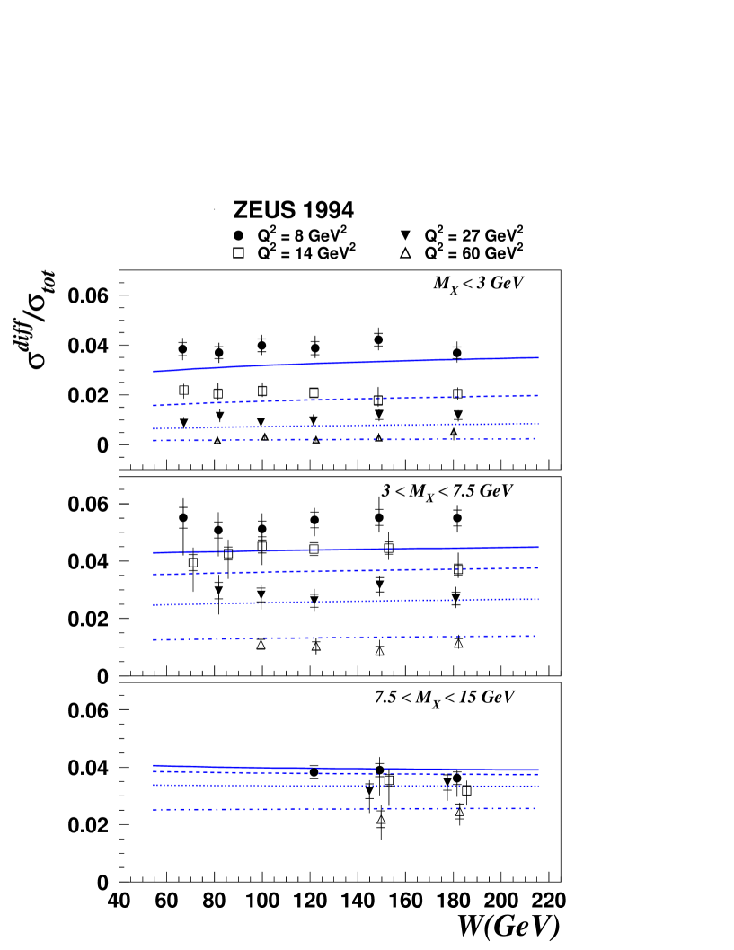
Figure 12: The ratio of the diffractive versus the inclusive cross sections as a function of $W$ for different values of $Q^{2}$ and the diffractive mass $M_{X}$.

In Fig. 12 we show the ratio of the diffractive versus inclusive cross section as a function of $W$ for different values of $Q^{2}$ and the diffractive mass $M$, in analogy to the analysis in Ref. [8]. Thus for the presented analysis we have integrated Eqs. (4), (4), (4) over the $\beta-$values which correspond to the indicated ranges of $M$. The values of the inclusive cross section were taken from the analysis in Ref. [1]. The ratio is almost constant over the entire range of $Q^{2}$ and $W$ with a slight growth at small $M$ caused by the longitudinal higher twist contribution. One can extract this behavior directly from the leading twist contributions of Eqs. (4) and (4) by simultaneous rescaling of the $l^{2}$- and $k^{2}$-integration with respect to $R_{0}^{2}$. We have already discussed that the constant ratio is a particular feature of our saturation model and certainly deviates from the ‘conventional’ triple Regge approach.

6 Diffractive structure function in impact parameter space representation

We have started our discussion in impact parameter space because it provides a natural way to formulate saturation. For this reason we re-derive the formulae of Section 5 in impact parameter space. Moreover, the dipole formulation has its natural foundation in impact parameter space [23, 24]. A simple $q\bar{q}$-pair represents an elementary color dipole which has an effective scattering cross section depending on the separation between the quark and antiquark.

We will briefly recall the wave function description for a $q\bar{q}$-pair in impact parameter space using the conventions of Ref. [25] where the subscript $(\pm,\pm)$ denotes the photon- and quark helicity (complex notation):

$$\psi_{(+,+)}({\bf r},\alpha) = \frac{\sqrt{2}\;i\;e}{2\pi}\;\alpha\;\sqrt{\alpha(1-\alpha)Q^{2}}\;K_{1}(\sqrt{\alpha(1-\alpha)Q^{2}r^{2}})\;\frac{{\bf r}}{r}$$

$$\psi_{(+,-)}({\bf r},\alpha) = \frac{\sqrt{2}\;i\;e}{2\pi}\;(1-\alpha)\;\sqrt{\alpha(1-\alpha)Q^{2}}\;K_{1}(\sqrt{\alpha(1-\alpha)Q^{2}r^{2}})\;\frac{{\bf r}}{r}$$ (27)

$$\psi_{(-,+)}({\bf r},\alpha) = \frac{\sqrt{2}\;i\;e}{2\pi}\;(1-\alpha)\;\sqrt{\alpha(1-\alpha)Q^{2}}\;K_{1}(\sqrt{\alpha(1-\alpha)Q^{2}r^{2}})\;\frac{{\bf r}^{*}}{r}$$

$$\psi_{(-,-)}({\bf r},\alpha) = \frac{\sqrt{2}\;i\;e}{2\pi}\;\alpha\;\sqrt{\alpha(1-\alpha)Q^{2}}\;K_{1}(\sqrt{\alpha(1-\alpha)Q^{2}r^{2}})\;\frac{{\bf r}^{*}}{r}\;\;.$$

$K_{1}$ is the MacDonald-Bessel function, and the variable ${\bf r}$ is conjugate to ${\bf k}_{t}$, i.e.

$$\psi({\bf r},\alpha) = \int\frac{d^{2}{\bf k}_{t}}{(2\pi)^{2}}\;e^{i\;{\bf k}_{t}\cdot{\bf r}}\;\psi({\bf k}_{t},\alpha)\;\;.$$ (28)

The longitudinal wave function reads:

$$\psi_{(0,\pm)}({\bf r},\alpha) = \frac{e}{\pi}\;\alpha(1-\alpha)\;Q\;K_{0}(\sqrt{\alpha(1-\alpha)Q^{2}r^{2}})\;\;.$$ (29)

The $\beta$-integrated diffractive structure function can now be readily expressed in terms of the above wave function and the effective dipole cross section $\hat{\sigma}$ [10, 11]:

$$F_{\{t,q\bar{q}\}}^{D}(Q^{2},x) = \frac{3Q^{2}}{128\pi^{5}B_{D}}\;\sum_{f}e_{f}^{2}\;\int_{0}^{1}d\alpha\;[\alpha^{2}+(1-\alpha)^{2}]\;\;$$

$$\times \alpha(1-\alpha)\;Q^{2}\;\int d^{2}{\bf r}\;K_{1}^{2}(\sqrt{\alpha(1-\alpha)Q^{2}r^{2}})\;\hat{\sigma}^{2}(r,x)$$

and

$$F_{\{l,q\bar{q}\}}^{D}(Q^{2},x) = \frac{3Q^{2}}{32\pi^{5}B_{D}}\;\sum_{f}e_{f}^{2}\;\int_{0}^{1}d\alpha\;\alpha(1-\alpha)\;\;$$

$$\times \alpha(1-\alpha)\;Q^{2}\;\int d^{2}{\bf r}\;K_{0}^{2}(\sqrt{\alpha(1-\alpha)Q^{2}r^{2}})\;\hat{\sigma}^{2}(r,x)\;\;.$$

These two equation demonstrate the simplification one achieves in impact parameter space provided the distributions are totally integrated. They have already been quoted in Eq. (8) rewritten as diffractive cross section. The disadvantage, however, is that for differential distributions which depend on final state energies one has to transform back to momentum space as in the case of the $\beta$-dependent structure function

$$x_{I\!\!P}F_{\{t,q\bar{q}\}}^{D}(Q^{2},\beta,x_{I\!\!P}) = \frac{3}{64\pi^{5}B_{D}}\;\sum_{f}e^{2}_{f}\;\frac{\beta^{2}}{(1-\beta)^{3}}\;\int\frac{d^{2}{\bf k}_{t}}{(2\pi)^{2}}\;\;k_{t}^{4}\;\;$$

$$\times \frac{1-\frac{2\beta}{1-\beta}\frac{k_{t}^{2}}{Q^{2}}}{\sqrt{1-\frac{4\beta}{1-\beta}\frac{k_{t}^{2}}{Q^{2}}}}\;\Theta\left(1-\frac{4\beta}{1-\beta}\frac{k_{t}^{2}}{Q^{2}}\right)\;\;$$

$$\times \int d^{2}{\bf r}\;\int d^{2}{\bf r}^{\prime}\;\;e^{i\;{\bf k}_{t}\cdot({\bf r}-{\bf r}^{\prime})}\;\;\hat{\sigma}(r,x_{I\!\!P})\;\hat{\sigma}(r^{\prime},x_{I\!\!P})\;\;$$

$$\times \frac{{\bf r}\cdot{\bf r}^{\prime}}{r\;r^{\prime}}\;K_{1}\left(\sqrt{\frac{\beta}{1-\beta}k_{t}^{2}r^{2}}\right)\;K_{1}\left(\sqrt{\frac{\beta}{1-\beta}k_{t}^{2}r^{\prime 2}}\right)\;.$$

We have made use of Eq. (22) to substitute $\alpha$ by $\beta$ keeping $k_{t}$ fixed. For the longitudinally polarized photons we find

$$x_{I\!\!P}F_{\{l,q\bar{q}\}}^{D}(Q^{2},\beta,x_{I\!\!P}) = \frac{3}{16\pi^{5}B_{D}}\;\sum_{f}e^{2}_{f}\;\frac{\beta^{3}}{(1-\beta)^{4}}\;\int\frac{d^{2}{\bf k}_{t}}{(2\pi)^{2}}\;\;k_{t}^{4}\;\;$$

$$\times \frac{{k_{t}^{2}}/{Q^{2}}}{\sqrt{1-\frac{4\beta}{1-\beta}\frac{k_{t}^{2}}{Q^{2}}}}\;\Theta\left(1-\frac{4\beta}{1-\beta}\frac{k_{t}^{2}}{Q^{2}}\right)\;\;$$

$$\times \int d^{2}{\bf r}\;\int d^{2}{\bf r}^{\prime}\;\;e^{i\;{\bf k}_{t}\cdot({\bf r}-{\bf r}^{\prime})}\;\;\hat{\sigma}(r,x_{I\!\!P})\;\hat{\sigma}(r^{\prime},x_{I\!\!P})\;\;$$

$$\times \;K_{0}\left(\sqrt{\frac{\beta}{1-\beta}k_{t}^{2}r^{2}}\right)\;K_{0}\left(\sqrt{\frac{\beta}{1-\beta}k_{t}^{2}r^{\prime 2}}\right)\;.$$

This contribution is suppressed by an extra power in $Q^{2}$ and therefore is a higher twist contribution. By using Eq. (4) one can directly transform Eqs. (6) and (6) into Eqs. (4) and (4).

It should be noted that, when Eqs. (6) and (6) are integrated over $\beta$, the argument $x_{I\!\!P}$ in $\hat{\sigma}$ is simply substituted by $x$. This procedure is valid in the high energy approach as long as the dominant contribution is not concentrated at small $\beta$. The $\beta$-integration then leads from Eqs. (6) and (6) back to Eqs. (6) and (6). In the case of a gluon in the final state one can no longer do a simple substitution but has to integrate the argument of $\hat{\sigma}$ explicitly.

We will discuss the impact parameterization of the $q\bar{q}g$-final state in more detail. Our starting point is the wave function for the effective gluon dipole as described in [13] (we use in this case the vector notation $\mbox{\bf k}_{t}=(k_{t}^{1},k_{t}^{2})$ and $m,n=1,2$

$$\psi^{mn}(\alpha,{\bf k}_{t}) = \frac{1}{\sqrt{\alpha(1-\alpha)Q^{2}}}\;\frac{k_{t}^{2}\;\delta^{mn}\;-\;2\;{\bf k}_{t}^{m}{\bf k}_{t}^{n}}{k_{t}^{2}+\alpha(1-\alpha)Q^{2}}$$

$$= \frac{1}{\sqrt{\alpha Q^{2}}}\;\frac{k_{t}^{2}\;\delta^{mn}\;-\;2\;{\bf k}_{t}^{m}{\bf k}_{t}^{n}}{k_{t}^{2}+\alpha Q^{2}}$$

The second line of the previous equation is a consequence of the strong ordering condition which implies $\alpha\ll 1$. The variable $\alpha$ has been introduced in analogy to Eq. (22) and is identical to ${zk_{t}^{2}}/{(1-z)Q^{2}}$,

$$\alpha Q^{2} = \frac{zk_{t}^{2}}{1-z}\;=\;zk^{2}\;\;,$$ (35)

where $k_{t}$ is the gluon transverse momentum in this case and $k^{2}$ describes the mean virtuality of the gluon in the upper $t$-channel.

The following relation illuminates the use of the wave function in momentum space. After the integration over the azimuth angle of $l_{t}$ one arrives at the core expression of Eq. (4)

$$\int\frac{d^{2}{\bf l}_{t}}{\pi l_{t}^{2}}\;\alpha_{s}{\cal F}(x_{I\!\!P},l_{t}^{2})\;\left[2\;\psi^{mn}(\alpha,{\bf k}_{t})\;-\;\psi^{mn}(\alpha,{\bf k}_{t}+{\bf l}_{t})\;-\;\psi^{mn}(\alpha,{\bf k}_{t}-{\bf l}_{t})\right]$$

$$= \int\frac{dl_{t}^{2}}{l_{t}^{2}}\;\frac{\alpha_{s}{\cal F}(x_{I\!\!P},l_{t}^{2})}{\sqrt{\alpha Q^{2}}}\left[1-\frac{2k_{t}^{2}}{k_{t}^{2}+\alpha Q^{2}}-\frac{l_{t}^{2}}{k_{t}^{2}}-\frac{\alpha Q^{2}}{k_{t}^{2}}\right.$$

$$\left.\hskip 113.81102pt+\;\frac{[l_{t}^{2}-k_{t}^{2}+\alpha Q^{2}]^{2}+2k_{t}^{2}\alpha Q^{2}}{k_{t}^{2}\sqrt{[l_{t}^{2}+k_{t}^{2}+\alpha Q^{2}]^{2}-4l_{t}^{2}k_{t}^{2}}}\right]\left\{2\frac{{\bf k}_{t}^{m}{\bf k}_{t}^{n}}{k_{t}^{2}}-\delta^{mn}\right\}$$

$$= \int\frac{dl_{t}^{2}}{l_{t}^{2}}\;\frac{\alpha_{s}{\cal F}(x_{I\!\!P},l_{t}^{2})}{(1-z)\sqrt{zk^{2}}}\left[z^{2}+(1-z)^{2}+\frac{l_{t}^{2}}{k^{2}}\right.$$

$$\left.\hskip 113.81102pt-\;\frac{[(1-2z)k^{2}-l_{t}^{2}]^{2}+2z(1-z)k^{4}}{k^{2}\sqrt{(l_{t}^{2}+k^{2})^{2}-4(1-z)\;l_{t}^{2}\;k^{2}}}\right]\left\{\delta^{mn}-2\frac{{\bf k}_{t}^{m}{\bf k}_{t}^{n}}{k_{t}^{2}}\right\}\;\;.$$

The four terms $\psi^{mn}(\alpha,{\bf k}_{t})+\psi^{mn}(\alpha,{\bf k}_{t})-\psi^{mn}(\alpha,{\bf k}_{t}+{\bf l}_{t})-\psi^{mn}(\alpha,{\bf k}_{t}-{\bf l}_{t})$ represent the four possible ways of coupling the two $t$-channel gluons to the gluon dipole (without crossing in the $t$-channel). The Fourier transformation of the wave function leads to

$$\psi^{mn}(\alpha,{\bf r}) = -\frac{1}{2\pi}\left(\delta^{mn}-2\frac{{\bf r}^{m}{\bf r}^{n}}{r^{2}}\right)\;\sqrt{\alpha Q^{2}}\;K_{2}(\sqrt{\alpha Q^{2}r^{2}})\;\;.$$ (37)

Inserting the Fourier transform into the first line of Eq. (6) and using Eq. (4) we find

$$\int\frac{d^{2}{\bf l}_{t}}{\pi l_{t}^{2}}\;\alpha_{s}{\cal F}(x_{I\!\!P},l_{t}^{2})\;\left[2\;\psi^{mn}(\alpha,{\bf k}_{t})\;-\;\psi^{mn}(\alpha,{\bf k}_{t}+{\bf l}_{t})\;-\;\psi^{mn}(\alpha,{\bf k}_{t}-{\bf l}_{t})\right]$$

$$= \int d^{2}{\bf r}\;\psi^{mn}(\alpha,{\bf r})\;\;e^{i\;{\bf k}_{t}\cdot{\bf r}}\;\int\frac{d^{2}{\bf l}_{t}}{\pi l_{t}^{2}}\;\alpha_{s}{\cal F}(x_{I\!\!P},l_{t}^{2})\;\left(2-e^{i\;{\bf l}_{t}\cdot{\bf r}}-e^{-i\;{\bf l}_{t}\cdot{\bf r}}\right)$$

$$= 2\;\int d^{2}{\bf r}\;\psi^{mn}(\alpha,{\bf r})\;\;e^{i\;{\bf k}_{t}\cdot{\bf r}}\;\frac{3}{4\pi^{2}}\;\hat{\sigma}(x_{I\!\!P},r)\;\;.$$

We can now rewrite Eq. (4) in impact parameter space as

$$x_{I\!\!P}F_{\{t,q\bar{q}g\}}^{D}(Q^{2},\beta,x_{I\!\!P}) = \frac{81\;\beta}{512\pi^{5}B_{D}}\;\sum_{f}e_{f}^{2}\;\frac{\alpha_{s}}{2\pi}\;\int_{\beta}^{1}\frac{dz}{z}\;\left[\left(1-\frac{\beta}{z}\right)^{2}\;+\;\left(\frac{\beta}{z}\right)^{2}\right]\;\frac{z}{(1-z)^{3}}\;$$

$$\times \int\frac{d^{2}{\bf k}_{t}}{(2\pi)^{2}}\;k_{t}^{4}\;\ln\left(\frac{(1-z)Q^{2}}{k_{t}^{2}}\right)\;\Theta\left[(1-z)Q^{2}-k_{t}^{2}\right]\;\;$$

$$\times \int d^{2}{\bf r}\;\int d^{2}{\bf r}^{\prime}\;\;e^{i\;{\bf k}_{t}\cdot({\bf r}-{\bf r}^{\prime})}\;\;\hat{\sigma}(r,x_{I\!\!P})\;\hat{\sigma}(r^{\prime},x_{I\!\!P})\;\left(\delta^{mn}-2\frac{{\bf r}^{m}{\bf r}^{n}}{r^{2}}\right)\;\;$$

$$\times \left(\delta^{mn}-2\frac{{\bf r}^{\prime m}{\bf r}^{\prime n}}{r^{\prime 2}}\right)\;K_{2}\left(\sqrt{\frac{z}{1-z}k_{t}^{2}r^{2}}\right)\;K_{2}\left(\sqrt{\frac{z}{1-z}k_{t}^{2}r^{\prime 2}}\right)$$

Again, a direct computation of Eq. (6) after substituting $\hat{\sigma}$ according to Eq. (4) reproduces the result of Eq. (4).

The impact parameter representation in Eqs. (6) and (6) demonstrate the similarity of our approach and the semiclassical approach of Ref. [26]. It suggests that the two-gluon exchange model can be extended to multi-gluon exchange without changing the basic analytic structure. The leading color tensors in the limit of large N_c (number of colors) for a quark- and a gluon-loop with an arbitrary number of $t$-channel gluons attached to them are found to be identical up to an overall constant factor [27]. The large N_c result differs only slightly from N${}_{c}=3$ in the two-gluon exchange model and, hence, multi-gluon exchange is expected to give very similar results as the two-gluon exchange.

7 Conclusions

In our analysis we successfully describe diffractive deep inelastic scattering using the saturation model proposed in Ref. [1]. This model reproduces quite accurately the $\beta$- and $x_{I\!\!P}$- distributions as measured by H1 and ZEUS [7, 8] without tuning or fitting any additional parameters.

As demonstrated in Ref. [1] saturation naturally explains the transition of the inclusive structure function $F_{2}$ from high to low values of $Q^{2}$. Diffractive scattering is even more effected by saturation (see Section 3). The constant ratio of the diffractive versus inclusive cross sections as observed at HERA is a direct consequence of saturation. It was also pointed out that soft contributions are significantly suppressed leading to a relative enhancement of semi-hard contributions. This fact allows the conclusion that diffraction in deep inelastic scattering is a semi-hard process [6]. The effective Pomeron intercept is higher than expected from a ‘soft’ Pomeron approach [7, 28]. The $\beta$-spectrum depends only weakly on the model and is therefore more universal.

The model we choose for saturation is purely phenomenological. An alternative model without low-$x$ saturation can be found in Ref. [31]. A completely theoretical framework involves non-linear QCD evolution equations as proposed in Refs. [2, 5, 30]. We believe, however, that our model represents the basic dynamics at very low $x$, since it allows us to describe a wide range of data in a satisfactory way.

We can use our analysis to predict diffractive charm production. This requires the discussion of factorization, the introduction of diffractive parton distributions and the evolution of the diffractive final state. The detailed discussion of these topics will be presented elsewhere [32].

Acknowledgements

We thank H. Abramowicz, C. Ewerz, J. Forshaw, G. Kerley, J. Kwiecinski, E. Levin, M. McDermott, G. Shaw and A. Stasto for useful discussions. H. Kowalski, P. Newman kindly provided us with the data from ZEUS and H1. We are particular grateful to H. Kowalski for his help in preparing Fig. 11 and Fig. 12. K.G-B. thanks the Department of Physics of the University of Durham for hospitality. This research has also been supported in part by the Polish State Committee for Scientific Research grant No. 2 P03B 089 13 and by the EU Fourth Framework Programme ‘Training and Mobility of Researchers’ Network, ‘Quantum Chromodynamics and the Deep Structure of Elementary Particles’, contract FMRX-CT98-0194 (DG 12-MIHT).

Appendix

In this appendix we would like to recall the derivation of Eq. (4) which represents the contribution due to the emission of an additional gluon [29]. We choose light-cone gauge with the gauge fixing condition $q^{\prime}\cdot A=0$ ($A$ is the gluon potential, $q^{\prime}=q+xp$). The frame which naturally corresponds to this choice of gauge is the Breit frame, i.e. the frame in which the proton is fast moving. All quasi-Bremsstrahlungs gluons emitted from the $q\bar{q}$-pair can be neglected. Those from the incoming partons on the other hand have to be taken into account.

The polarization vector $\epsilon$ for real gluons and the polarization tensor for the gluon propagator $d^{\nu\mu}$ read:

$$\epsilon^{\mu}(k) = \epsilon_{t}^{\nu}(k)-q^{\prime\mu}\;\frac{k_{t}\cdot\epsilon_{t}(k)}{k\cdot q^{\prime}}$$ (40)

$$d^{\nu\mu}(k) = g^{\nu\mu}-\frac{k^{\nu}q^{\prime\mu}+q^{\prime\nu}k^{\mu}}{k\cdot q^{\prime}}\;\;.\$$

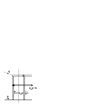
Figure 4: Gluon radiation.

Figure 4 shows all the essential diagrams. The two diagrams to the left have a similar momentum structure and will be summed up right from the beginning whereas the diagram on the right will be calculated separately. The bottom line in all the diagrams represents a quark. It is accompanied by other ’spectator-quarks’ which are not shown explicitly. The cut through the diagrams effectively subdivides the whole amplitude into two subprocesses. We will introduce effective three gluon couplings which are the sum of the original three gluon coupling and extra Bremsstrahlungs contributions (see Fig. 5). These couplings and their analytic formulae represent the core of the whole calculation. The blob at the top of the right $t$-channel gluon in Fig. 4 indicates the simultaneous coupling of the $t$-channel gluon to the $q\bar{q}$-pair which in color space combines into a gluon.

Before starting the calculation one has to recall and make use of the kinematic assumptions made in this approach. Firstly, there is the Regge limit with respect to the lower part of the diagram, i.e. the emitted gluon and the quark at the bottom have an invariant subenergy much larger than the diffractive mass $M$. The high energy assumption allows one to simplify the $t$-channel propagator as to

$$d^{\rho\sigma}(l+x_{I\!\!P}p) = g^{\rho\sigma}-\frac{(l+x_{I\!\!P}p)^{\rho}q^{\prime\sigma}+q^{\prime\rho}(l+x_{I\!\!P}p)^{\sigma}}{(\beta_{l}+x_{I\!\!P})p\cdot q^{\prime}}$$

$$\simeq -\frac{l_{t}^{\rho}q^{\prime\sigma}}{(\beta_{l}+x_{I\!\!P})p\cdot q^{\prime}}$$

where the index $\rho$ refers to the polarization at the upper end of the gluon line and $\sigma$ to the lower end. $\beta_{l}$ corresponds to the Sudakov decomposition $l=\beta_{l}p+\alpha_{l}q^{\prime}+l_{t}$ where $\alpha_{l}$ is fixed using the fact that the quark at the bottom is on-shell ($\alpha_{l}\simeq l^{2}_{t}/s$). $\beta_{l}$ itself is given through the on-shell condition of the intermediate $s$-channel gluon $(l+x_{I\!\!P}p-k)^{2}=0$ and the final state gluon $(x_{I\!\!P}p-k)^{2}=0$:

$$\beta_{l} = \frac{l_{t}^{2}-2l_{t}\cdot k_{t}}{\alpha_{k}s}$$ (42)

$$\alpha_{k} = \frac{k_{t}^{2}}{(x_{I\!\!P}-\beta_{k})s}$$

($s=2p\cdot q^{\prime}$). Here the Sudakov representation of $k$ enters with $\beta_{k}$ as free variable denoting the momentum fraction of the upper $t$-channel gluon with respect to the momentum $p$. Later on it will be substituted by $z$ ($z=\beta_{k}/x_{I\!\!P}$) which then denotes the momentum fraction of the $t$-channel gluon with respect to the Pomeron momentum. The contraction of $q^{\prime\sigma}$ with the lower quark-gluon vertex gives roughly $q^{\prime}\cdot p$ which cancels the same factor in the denominator of Eq. (Appendix). The remaining factor $1/(\beta_{l}+x_{I\!\!P}p)$ in front of the vector $l_{t}^{\rho}$ is large provided that $x_{I\!\!P}$ is small. The other components of the polarization tensor $d^{\rho\sigma}$ are negligible. All these properties are crucial in proving the $k_{t}$-factorization theorem. For the upper $t$-channel gluon the situation is different. In this case the corresponding tensor reads:

$$d^{\rho\sigma}(k) = g^{\rho\sigma}-\frac{k^{\rho}q^{\prime\sigma}+q^{\prime\rho}k^{\sigma}}{k\cdot q^{\prime}}$$

$$= g_{t}^{\rho\sigma}-\frac{k_{t}^{\rho}q^{\prime\sigma}+q^{\prime\rho}k_{t}^{\sigma}+2\alpha_{k}q^{\prime\rho}q^{\prime}\sigma}{\beta_{k}p\cdot q^{\prime}}$$

Due to the fact that the contraction of $q^{\prime\sigma}$ downwards gives a factor $x_{I\!\!P}p\cdot q^{\prime}$ which is not much larger than $\beta_{k}$, but of the same order, the term $\beta_{k}$ in the denominator of Eq. (Appendix) is no longer enhanced as in Eq. (Appendix). However, a simplification is still possible, if one restricts oneself to the calculation of leading twist terms and keeps only the leading logs in $Q^{2}$. Then, the transverse momenta of the quarks at the top of the diagram in Fig. 40 and the gluon below are strongly ordered and all contributions with an extra inverse power of the large quark transverse momentum are suppressed. This allows to set the transverse momentum $k_{t}$ along any of the quark lines to zero. Moreover, the projection of $q^{\prime\rho}$ with one of the upper quark-gluon vertices cancels or is sub-leading, and Eq. (Appendix) may be reduced to:

$$d^{\rho\sigma}(k)\;\simeq\;g_{t}^{\rho\sigma}-\frac{k_{t}^{\rho}q^{\prime\sigma}}{\beta_{k}p\cdot q^{\prime}}\;\;.$$ (44)

This kind of technique is well known and has been applied in deriving the conventional Altarelli-Parisi splitting function. Therefore it is not surprising that the production of the $q\bar{q}$-system is basically described by the AP-splitting function associated with the splitting of a gluon into two quarks accompanied by a logarithm in $Q^{2}/k_{t}^{2}$. Certainly, this approach is only valid for the transverse part of the cross section. The longitudinal part gives a next-to-leading log($Q^{2}$) contribution which is not considered here. The coupling of the second gluon to the $q\bar{q}$-system does not affect the dynamics within this system, but feels only the total color charge which is the same charge as carried by the first gluon.

Figure 5: Effective triple gluon couplings.

To summarize, the leading twist approach allows to factorize off the $q\bar{q}$-system analogously to the conventional leading order DGLAP-scheme whereas in the lower part the $k_{t}$-factorization theorem is applicable. All together, a local vertex may be extracted describing the transition between the lower Pomeron exchange and the upper QCD-radiation. It is useful to rewrite Eq. (44) in terms of transverse polarization vectors $\epsilon_{t}$ defined as

$$g_{t}^{\rho\sigma} = -\,\sum_{pol}\;\epsilon_{t}^{\rho}\epsilon_{t}^{\sigma}$$ (45)

$$(\epsilon_{t})_{i}\cdot(\epsilon_{t})_{j} = -\delta_{ij}\;\;.$$

The sum has to be taken over the two helicity or polarization configurations in the transverse plane. $d^{\rho\sigma}$ then reads:

$$d^{\rho\sigma}\;=\;\sum_{pol}\;\epsilon^{\rho}(k)\;\epsilon^{\sigma}(k)$$ (46)

with

$$\epsilon^{\sigma}(k)\;=\;\epsilon_{t}^{\sigma}\,-\,\frac{k_{t}\cdot\epsilon_{t}\,q^{\prime\sigma}}{\beta_{k}p\cdot q^{\prime}}\;\;.$$ (47)

Having in mind the previous discussion one can now start the calculation of the diagrams in Fig. 4. The effective triple gluon vertex to the left of the first diagram gives the following contribution:

$$2\;\;p\cdot\epsilon(k)\;\;l_{t}\cdot\epsilon(l+x_{I\!\!P}p-k)$$

$$- \frac{\beta_{l}\alpha_{k}s}{\beta_{l}+x_{I\!\!P}}\;\;\epsilon_{t}\cdot\epsilon(l+x_{I\!\!P}p-k)$$

$$- 2\;\;p\cdot\epsilon(l+x_{I\!\!P}p-k)\;\;l_{t}\cdot\epsilon_{t}$$

$$- 2\;\;p\cdot\epsilon(l+x_{I\!\!P}p-k)\;\;k_{t}\cdot\epsilon_{t}\;\frac{l_{t}^{2}}{\beta_{k}\alpha_{k}s}$$

The first three terms of Eq. (Appendix) result from the ordinary three gluon coupling whereas the last is the sum of the two Bremsstrahlungs gluons as illustrated in the first row of Fig. 5. The momentum structure of these contributions is the same except the overall sign which is opposite. It is obvious that the two color tensors add up to the same tensor the ordinary three gluon coupling has. The overall color factor will be evaluated later. Here, only the correspondence between different color tensors is of interest but not the whole tensor itself. The right effective vertex in the first diagram of Fig. 4 is different as it contains two $s$-channel gluons. Since these gluons are on-shell, the Ward identity $l^{\rho}A_{\rho}=0$, where $A^{\rho}$ is the triple gluon coupling contracted with the gluon polarization vectors, may be used to change the $t$-channel polarization vector from $l_{t}^{\rho}/\beta_{l}$ to $p^{\rho}$. The resulting expression is:

$$- 2\;\;l_{t}\cdot\epsilon(x_{I\!\!P}p-k)\;\;p\cdot\epsilon(l+x_{I\!\!P}p-k)$$

$$+ 2\;\;l_{t}\cdot\epsilon(l+x_{I\!\!P}p-k)\;\;p\cdot\epsilon(x_{I\!\!P}p-k)$$

$$- \alpha_{k}s\;\epsilon(l+x_{I\!\!P}p-k)\cdot\epsilon(x_{I\!\!P}p-k)$$

$$+ 2\;\;p\cdot\epsilon(l+x_{I\!\!P}p-k)\;\;p\cdot\epsilon(x_{I\!\!P}p-k)\;\frac{l_{t}^{2}}{\alpha_{k}s}\;\;.$$

Both pieces Eqs. (Appendix) and (Appendix) have to be combined and the sum over the transverse polarizations of the intermediate $s$-channel gluon has to be performed. The following equation will be used:

$$\sum_{pol}\;\epsilon_{t}^{\mu}(l+x_{I\!\!P}p-k)\,\epsilon_{t}^{\nu}(l+x_{I\!\!P}p-k)\;=\;-\;g_{t}^{\mu\nu}\;\;,$$ (50)

and products like $p\cdot\epsilon(k)$ will be reduced to $-2\,k_{t}\cdot\epsilon_{t}/\beta_{k}$. Furthermore, the propagator $1/k^{2}=x_{I\!\!P}/(\alpha_{k}s)=(1-z)/k_{t}^{2}$ is introduced and $\beta_{l}$ is expressed through Eq. (42) as well as the variable $\beta_{k}$ is substituted by $z$ ($\beta_{k}=x_{I\!\!P}z$):

$$-\,\frac{2}{x_{I\!\!P}}\;\frac{k_{t}\cdot\epsilon_{t}}{zk^{2}} \left\{-\,2\frac{l_{t}\cdot(l_{t}-k_{t})}{(l_{t}-k_{t})^{2}}\;\left[\frac{l_{t}^{2}}{k_{t}^{2}}k_{t}\cdot\epsilon(x_{I\!\!P}p-k)-l_{t}\cdot\epsilon(x_{I\!\!P}p-k)\right]\right.$$ (51)

$$\left.+\,2\,l_{t}^{2}\frac{k_{t}\cdot\epsilon(x_{I\!\!P}p-k)}{k_{t}^{2}}\,-\,l_{t}\cdot\epsilon(x_{I\!\!P}p-k)\right\}$$

$$-\,\frac{1}{x_{I\!\!P}}\left(1-\frac{k^{2}}{k^{2}+l_{t}^{2}-2l_{t}\cdot k_{t}}\right) \left\{-2\frac{(l_{t}-k_{t})\cdot\epsilon_{t}}{(l_{t}-k_{t})^{2}}\left[\frac{l_{t}^{2}}{k_{t}^{2}}k_{t}\cdot\epsilon(x_{I\!\!P}p-k)-l_{t}\cdot\epsilon(x_{I\!\!P}p-k)\right]\right.$$

$$\left.+\,2l_{t}\cdot\epsilon_{t}\frac{k_{t}\cdot\epsilon(x_{I\!\!P}p-k)}{k_{t}^{2}}\,-\,\epsilon_{t}\cdot\epsilon(x_{I\!\!P}p-k)\right\}$$

$$+\,\frac{2}{x_{I\!\!P}}\,\left[l_{t}\cdot\epsilon_{t}\,+\,\frac{1-z}{z}\frac{l_{t}^{2}}{k_{t}^{2}}\,k_{t}\cdot\epsilon_{t}\right] \left\{-\frac{2}{(l_{t}-k_{t})^{2}}\left[\frac{l_{t}^{2}}{k_{t}^{2}}k_{t}\cdot\epsilon(x_{I\!\!P}p-k)-l_{t}\cdot\epsilon(x_{I\!\!P}p-k)\right]\right.$$

$$\left.+\,2\,\frac{l_{t}\cdot(l_{t}-k_{t})}{(l_{t}-k_{t})^{2}}\frac{k_{t}\cdot\epsilon(x_{I\!\!P}p-k)}{k_{t}^{2}}\,-\,\frac{(l_{t}-k_{t})\cdot\epsilon(x_{I\!\!P}p-k)}{(l_{t}-k_{t})^{2}}\right\}$$

The next contribution has to be taken from the second diagram in Fig. 4. In this case the situation is slightly simpler compared to the first diagram, since only one effective triple gluon vertex appears. Moreover, the upper $t$-channel gluon is attached to a quark line where the incoming and the outgoing quarks are on-shell with the consequence that the momentum of this gluon is purely transverse up to corrections proportional to the squared ratio of the gluon transverse momentum and the quark transverse momentum. This type of correction is sub-leading due to the strong ordering assumption. The polarization tensor simplifies in the following way:

$$d^{\rho\sigma}(l+x_{I\!\!P}p-k)\;=\;\frac{p^{\rho}q^{\prime\sigma}}{p\cdot q^{\prime}}\;\;.$$ (52)

The upper polarization vector was changed from $-\frac{(l_{t}-k_{t})^{\rho}}{\beta_{l}+x_{I\!\!P}-\beta_{k}}$ to $p^{\rho}$ making use of the fact that the two quarks to the left and to the right are on-shell. In contrast to the first diagram in Figure 4 the tensor $g_{t}^{\rho\sigma}$ along the $t$-channel line gives only a sub-leading contributions due to the smallness of the longitudinal momentum. The special kinematic situation in the second diagram allows one to apply the eikonal approximation to the right quark-gluon vertex. The subsequent contraction with $p^{\rho}$ gives a factor which is cancelled by the residue of the $\delta$-function corresponding to the intermediate quark, and the remaining factor is simply $-1$. The softness of the upper right $t$-channel gluon has no further dynamical effect except that the color charge of both quarks add up to the total color charge of the left $t$-channel gluon. Consequently, the color factor is identical to that of the first diagram in Figure 4. After all, one finds for this diagram:

$$- \frac{2}{\beta_{k}}\;\;l_{t}\cdot\epsilon_{t}\;\;l_{t}\cdot\epsilon(x_{I\!\!P}p-k)$$

$$+ \frac{2}{\beta_{k}}\;\;l_{t}\cdot\epsilon_{t}\;\;\frac{l_{t}^{2}}{\alpha_{k}s}\;\;p\cdot\epsilon(x_{I\!\!P}p-k)$$

Inserting the propagator $1/(l_{t}-k_{t})^{2}$ and substituting $\beta_{k}$ as well as $\alpha_{k}$ one finally comes to:

$$\frac{2}{x_{I\!\!P}}\;\;\frac{1}{z}\;\;\frac{l_{t}\cdot\epsilon_{t}}{(l_{t}-k_{t})^{2}}\;\;\left[\frac{l_{t}^{2}}{k_{t}^{2}}\;k_{t}\cdot\epsilon(x_{I\!\!P}p-k)\;-\;l_{t}\cdot\epsilon(x_{I\!\!P}p-k)\right]$$ (54)

In the following step the two expressions (51) and (54) will be added and the result integrated over the azimuth angle between $l_{t}$ and $k_{t}$. A lot of cancellations occur and the final expression is rather short:

$$-\;\frac{1}{2x_{I\!\!P}}\;\frac{1}{z(1-z)} \left\{z^{2}\,+\,(1-z)^{2}\,+\,\frac{l_{t}^{2}}{k^{2}}\right.$$

$$\left.-\,\frac{\left[(1-2z)k^{2}-l_{t}^{2}\right]^{2}+2z(1-z)k^{4}}{k^{2}\sqrt{(k^{2}+l_{t}^{2})^{2}-4(1-z)l_{t}^{2}k^{2}}}\right\}\;\;\epsilon_{t}\cdot\epsilon_{t}(x_{I\!\!P}p-k)\;\;.$$

Recalling the fact that only the amplitude has been considered, the calculation of the cross section requires to take the square of Expr. (Appendix). In doing so one has to sum over the final state polarizations which leads to a contraction of the vector $\epsilon_{t}$ with its conjugate. In the end the transverse part of the $\gamma$-matrices in the lower edges of the quark-box are contacted as well (see Fig. 4).

Moving on to the final diagram (Fig. 4) one encounters a similar situation as in the case of the second diagram of the same figure. The right $t$-channel gluon is soft in the sense that its momentum is small compared to the quark momenta. It has no dynamical effect except that the color charge adds up as before, so that the final color factor is identical to that in the first two diagrams of Fig. 4. What remains is the calculation of the left effective triple gluon vertex. This has to be performed in a similar way as in the case of the left vertex in the second diagram:

$$2\;\;p\cdot\epsilon(l+k)\;\;l_{t}\cdot\epsilon(x_{I\!\!P}p-k)$$

$$+ \frac{l_{t}^{2}+2l_{t}\cdot k_{t}}{\beta_{l}+x_{I\!\!P}}\;\;\epsilon(l+k)\cdot\epsilon(x_{I\!\!P}p-k)$$

$$- 2\;\;p\cdot\epsilon(x_{I\!\!P}p-k)\;\;l_{t}\cdot\epsilon(l+k)$$

$$- 2\;\;p\cdot\epsilon(x_{I\!\!P}p-k)\;\;(l_{t}+k_{t})\cdot\epsilon(l+k)\;\frac{l_{t}^{2}}{(\beta_{l}+\beta_{k})\alpha_{k}s}$$

The last term in Eq. (Appendix) summarizes the contribution of the Bremsstrahlungs gluons associated with the effective triple gluon coupling. As was argued before the longitudinal momentum of the right soft $t$-channel gluon is negligible and $\beta_{l}$ equals zero. The momentum of the upper left $t$-channel gluon does not reduce to its transverse component, but includes the non-negligible longitudinal fraction $z$ of the Pomeron momentum. Therefore, the propagator $1/(l+k)^{2}$ transforms into $1/(zk^{2}+(l_{t}+k_{t})^{2})$. Introducing this propagator into Eq. (Appendix) and substituting $\beta_{k}=zx_{I\!\!P}$ as well as $\alpha_{k}s=k^{2}/x_{I\!\!P}$ one finds:

$$- \frac{2}{x_{I\!\!P}}\;\frac{1}{z}\;\frac{(l_{t}+k_{t})\cdot\epsilon(l+k)\;l_{t}\cdot\epsilon(x_{I\!\!P}p-k)}{zk^{2}+(l_{t}+k_{t})^{2}}$$

$$- \frac{2}{x_{I\!\!P}}\;\frac{1}{z}\;\frac{l_{t}^{2}}{k_{t}^{2}}\;\;\frac{(l_{t}+k_{t})\cdot\epsilon(l+k)\;k_{t}\cdot\epsilon(x_{I\!\!P}p-k)}{zk^{2}+(l_{t}+k_{t})^{2}}$$

$$- \frac{2}{x_{I\!\!P}}\;\frac{1}{1-z}\;\frac{l_{t}\cdot\epsilon(l+k)\;k_{t}\cdot\epsilon(x_{I\!\!P}p-k)}{zk^{2}+(l_{t}+k_{t})^{2}}$$

$$+ \frac{1}{x_{I\!\!P}}\;\frac{(l_{t}+k_{t})^{2}-k_{t}^{2}}{zk^{2}+(l_{t}+k_{t})^{2}}\;\;\epsilon(l+k)\cdot\epsilon(x_{I\!\!P}p-k)$$

Once more one has to integrate over the azimuth angle between $l_{t}$ and $k_{t}$ with the remarkable outcome that the resulting expression is identical to Eq. (Appendix):

$$-\;\frac{1}{2x_{I\!\!P}}\;\frac{1}{z(1-z)} \left\{z^{2}\,+\,(1-z)^{2}\,+\,\frac{l_{t}^{2}}{k^{2}}\right.$$

$$\left.-\,\frac{\left[(1-2z)k^{2}-l_{t}^{2}\right]^{2}+2z(1-z)k^{4}}{k^{2}\sqrt{(k^{2}+l_{t}^{2})^{2}-4(1-z)l_{t}^{2}k^{2}}}\right\}\;\;\epsilon_{t}\cdot\epsilon_{t}(x_{I\!\!P}p-k)\;\;.$$

In other words, the sum of the first two diagrams in Fig. 4 is identical to the third diagram bearing in mind that the light cone gauge with the condition $q^{\prime}\cdot A=0$ was used. One should remind that the amplitude was calculated in the high energy asymptotic region where the real parts of the $s$-channel and $u$-channel contributions cancel due to the even signature of the color singlet exchange. (The $u$-channel contribution corresponds to the crossing of the two lower $t$-channel gluons in Fig. 4.). Hence, the imaginary part gives the leading part and was calculated taking the $s$-channel discontinuity, i.e. cutting the diagrams. However, the cut diagram gives twice the imaginary part and one has to divide the final result by 2.

The structure in Eq. (Appendix) has been used in Eq. (4). The wave function in Eq. (6) cannot be extracted directly from the diagrams discussed here, but was constructed such that it reproduces the same results.

Figure 7: The diffractive structure function $x_{{I\!\!P}}F^{D}(x_{{I\!\!P}},\beta,Q^{2})$ for $x_{{I\!\!P}}=0.0042$ as a function of $\beta$. The dashed lines show the $q\bar{q}$ contribution for transverse photons (4), the dot-dashed lines correspond to the contribution from longitudinal photons (4) and the dotted lines illustrate the $q\bar{q}g$ component (4). The solid line is the total contribution and the data are from ZEUS.

Figure 8: The same comparison as in Fig. 7 but with H1 data. Only the total contribution is shown (solid lines).

Figure 9: The diffractive structure functions $x_{{I\!\!P}}F^{D}(x_{{I\!\!P}},\beta,Q^{2})$ as measured by ZEUS plotted as a function of $x_{{I\!\!P}}$ for different values of $\beta$ and $Q^{2}$ (in units of $GeV^{2}$).

References

[1] K. Golec-Biernat, M. Wüsthoff,
Phys. Rev. D59 (1999) 014017.
[4] A. L. Ayala, M. B. Gay Ducati, E. M. Levin,
Nucl.Phys. B493 (1997) 305.
[5] J. Jalilian-Marian, A. Kovner, A. Leonidov, H. Weigert,
Phys. Rev. D59 (1999) 034007.
[6] A.H. Mueller, Eur. Phys. J. A1 (1998) 19;
Proceedings of the International Workshop
on Deep Inelastic Scattering and QCD (DIS 98), Brussels, Belgium, 4-8 Apr. 1998.
[7] H1 Collab., C. Adloff et al., Z. Phys. C76 (1997) 613.
[8] ZEUS Collab., J. Breitweg et al., Eur. Phys. J. C6 (1999) 43.
[9] N.Nikolaev, B.G.Zakharov, Z. Phys. C49 (1990) 607.
[10] J.R. Forshaw and D.A. Ross, QCD and the Pomeron,
Cambridge University Press, 1996.
[11] N.Nikolaev, B.G.Zakharov, Z. Phys. C53 (1992).
[12] J. Bartels, H. Jung, M. Wüsthoff, hep-ph/9903265, preprint
DESY-99-027, DTP/99/10, LUNFD6/(NFFL-7166).
[13] M. Wüsthoff, Phys. Rev. D56 (1997) 4311.
[14] F. Hautmann, Z. Kunszt, D.E. Soper, Phys. Rev. Lett. 81 (1998) 3333.
[15] M.G. Ryskin, Sov. J. Nucl. Phys. 52 (1990) 529.
[17] E. Levin, M. Wüsthoff, Phys.Rev. D50 (1994) 4306.
[18] E. Gotsman, E. Levin, U. Maor, Nucl. Phys. B493 (1997) 354.
[19] H1 Collab., S. Aid et al., Nucl. Phys. B470 (1996) 399;
H1 Collab., C. Adloff et al., Nucl. Phys. B497 (1997) 3.
[20] ZEUS Collab., M. Derrick et al., Z. Phys. C72 (1996) 399;
ZEUS Collab., M. Derrick et al., preprint DESY-98-121.
[21] ZEUS Collab., J. Breitweg et al., Eur. Phys. J. C1 (1998) 81.
[22] J. Bartels, J. Ellis, H. Kowalski, M. Wüsthoff,
hep-ph/9803497, to be published in Eur. Phys. J. C.
[23] A.H. Mueller and B. Patel, Nucl. Phys. B425 (1994) 471.
[24] A. Bialas, R. Peschanski, Phys. Lett. B378 (1996) 302.
[25] D.Yu. Ivanov, M. Wüsthoff, hep-ph/9808455,
to be published in Eur. Phys. J. C.
[26] W. Buchmüller, T. Gehrmann and A. Hebecker,
Nucl. Phys. B537 (1999) 477.
[27] C. Ewerz, PhD-thesis, preprint DESY-THESIS-1998-025.
[28] G. Ingelman and P. Schlein, Phys. Lett. B152 (1985) 256;
A. Capella et al., Phys. Lett. B343 (1995) 403;
K. Golec-Biernat and J. Kwiecinski, Phys. Lett. B353 (1995) 329;
T. Gehrmann and W.J. Stirling, Z. Phys. C70 (1996) 89.
[29] M. Wüsthoff, PhD-thesis, preprint DESY-95-166.
[30] Y.V. Kovchegov, hep-ph/9901281;
Y.V. Kovchegov and L. McLerran, hep-ph/9903246.
[31] J. Forshaw, G. Kerley and G. Shaw, hep-ph/9903341.
[32] K. Golec-Biernat, M. Wüsthoff, preprint in preparation.