Minimal Gauge Invariant Classes of Tree Diagrams in Gauge Theories

Abstract

We describe the explicit construction of groves, the smallest gauge invariant classes of tree Feynman diagrams in gauge theories. The construction is valid for gauge theories with any number of group factors which may be mixed. It requires no summation over a complete gauge group multiplet of external matter fields. The method is therefore suitable for defining gauge invariant classes of Feynman diagrams for processes with many observed final state particles in the standard model and its extensions.

I Introduction

The quest for a theory of flavor demands precise calculations of high energy scattering processes in the framework of the standard model and its extensions. At the Tevatron, the LHC, and at a future $e^{+}e^{-}$ Linear Collider, final states with many detected particles and tagged flavor will be the primary handle for testing theories of flavor. Calculations of cross section with many particle final states remain challenging and it is of crucial importance to be able to concentrate on the important parts of the scattering amplitude for the phenomena under consideration.

In gauge theories, however, it is impossible to simply select the signal diagrams and to ignore irreducible backgrounds. The same subtle cancellations among the diagrams in a gauge invariant subset that lead to the celebrated good high energy behavior of gauge theories such as the standard model, come back to haunt us if we accidentally select a subset of diagrams that is not gauge invariant. The results from such a calculation have no predictive power, because they depend on unphysical parameters introduced during the gauge fixing of the Lagrangian. It must be stressed that not all diagrams in a gauge invariant subset have the same pole structure and that a selection based on ‘signal’ or ‘background’ will not suffice.

The subsets of Feynman diagrams selected for any calculation must therefore form a gauge invariant subset, i. e. together they must already satisfy the Ward and Slavnov-Taylor identities to insure the cancellation of contributions from unphysical degrees of freedom.

In abelian gauge theories, such as QED, the classification of gauge invariant subsets is straightforward and can be summarized by the requirement of inserting any additional photon into all connected charged propagators. This situation is similar for gauge theories with simple gauge groups, the difference being that the gauge bosons are carrying charge themselves. For non-simple gauge groups like the standard model, which even includes mixing, the classification of gauge invariant subsets is much more involved.

Indeed, up to now, the classification of gauge invariant subsets in the standard model has been performed in an ad-hoc fashion (cf. [1, 2]). In this note we present an explicit construction of groves, the smallest gauge invariant classes of tree Feynman diagrams in gauge theories. Our construction is not restricted to gauge theories with simple gauge groups. Instead, it is applicable to gauge groups with any number of factors, which can even be mixed, as in the standard model. Furthermore, it does not require a summation over complete multiplets and can therefore be used in flavor physics when members of weak isospin doublets (such as charm or bottom) are detected separately. Our method constructs the smallest gauge invariant subsets. Below we show examples in which they are indeed smaller than those derived from looking at final state alone [1, 2].

We expect that our methods will also have applications in loop calculations. However, some of our current proofs use properties of tree diagrams and further research is required in this area.

II Forests

We introduce basic notions in the case of unflavored scalar $\phi^{3}$- and $\phi^{4}$-theory. In the absence of selection rules, the diagrams $S_{1}$, $S_{2}$, and $S_{3}$ in figure 1 must have the same coupling strength to ensure crossing invariance. If there are additional symmetries, as in the case of gauge theories, the coupling of $S_{4}$ will be fixed relative to $S_{1,2,3}$.

The elementary flips $S_{t_{4}}\to S_{t^{\prime}_{4}}$ define relations $t_{4}\circ t^{\prime}_{4}$ on the set $T_{4}$ of all tree graphs with four external particles. These trivial relations have a non-trivial natural extension to the set $T(E)$ of all tree diagrams with a given external state $E$ by

$$t\circ t^{\prime}\Longleftrightarrow\exists t_{4}\in T_{4},t^{\prime}_{4}\in T_{4}:t_{4}\circ t^{\prime}_{4}\land t\setminus t_{4}=t^{\prime}\setminus t^{\prime}_{4},$$ (1)

i. e. two diagrams satisfy the relation if they are identical up to a single flip of a four-point subdiagram. This relation allows to view the set $T(E)$ of all tree diagrams as the vertices of a graph $F(E)$

$$F(E)=\bigl{\{}(t,t^{\prime})\in T(E)\times T(E)\bigl{|}t\circ t^{\prime}\bigl{\}},$$ (2)

where the edges of the graph are formed by the pairs of diagrams related by a single flip. To avoid confusion, we will refer to graph $F(E)$ as forest and to its vertices as Feynman diagrams. For lack of space, we have to introduce some mathematical concepts rather tersely and will give a more self-contained presentation elsewhere [3].

Already the simplest non-trivial example of such a forest, the 15 tree diagrams with five external particles in unflavored $\phi^{3}$-theory, as shown in figure 2, displays an intriguing structure. The most important property for our applications is

Theorem 1

The unflavored forest $F(E)$ is connected for all external states $E$,

which is easily proved by induction on the number of particles in the external state. This theorem shows that it is possible to construct all Feynman diagrams by visiting the nodes of $F(E)$ along successive applications of the flips in figure 1.

III Flavored Forests

In physics applications we have to deal with different particles. Therefore we introduce flavored forests, where the admissibility of elementary flips $t_{4}\circ t_{4}^{\prime}$ depends on the four particles involved through the Feynman rules for the vertices in $t_{4}$ and $t_{4}^{\prime}$. Flavored forests have in general more than one connected component.

In order to simplify the combinatorics when counting diagrams for theories with more than one flavor, we will below treat all external particles as outgoing. The physical amplitudes are obtained later by selecting the incoming particles in the end. Ward identities, etc. will be proved for the latter physical amplitudes, of course.

IV Groves

Our method is based on the observation that the flips in gauge theories fall into two different classes: the flavor flips in figure 3 which involve four matter fields which carry gauge charge and possibly additional conserved quantum numbers and the gauge flips in figures 4 and 5 which also involve gauge bosons (another diagram, $t_{4}^{G,8}\propto\phi^{2}A^{2}$, has to be added for scalar matter fields that appear in extensions of the standard model: SUSY partners, leptoquarks, etc.). In gauge theories with more than one factor, like the standard model, the gauge flips are extended in the obvious way to include all four-point functions with at least one gauge-boson. Commuting gauge group factors lead to separate sets, of course. In spontaneously broken gauge theories, the Higgs and Goldstone boson fields contribute additional flips, in which they are treated like gauge bosons (see [3] for a complete list and applications). Ghosts can be ignored at tree level.

The flavor flips (figure 3) are special because they can be switched off without spoiling gauge invariance by introducing a horizontal symmetry that commutes with the gauge group. Such a horizontal symmetry is similar to the replicated generations in the standard model, but if three generations do not suffice, it can also be introduced artificially. Typical examples are Bhabha-scattering, where the $s$-channel and the $t$-channel diagrams are separately gauge invariant, because we can replace one electron line by a muon line without violating gauge invariance. Similarly, the charged current and neutral current contributions in $ud\to ud$ can be switched on and off by assuming that two of the four quarks are from a different generation.

This observation suggests to introduce two relations:

$$t\bullet t^{\prime}\Longleftrightarrow\text{{\hbox{t}} and~{}{\hbox{t'}} related by a \emph{gauge} flip}$$ (3)

and

$$t\circ t^{\prime}\Longleftrightarrow\text{{\hbox{t}} and~{}{\hbox{t'}} related by a \emph{flavor or gauge} flip}.$$ (4)

These two relations define two different graphs with the same set $T(E)$ of all Feynman diagrams as vertices:

$$F(E)=\bigl{\{}(t,t^{\prime})\in T(E)\times T(E)\bigl{|}t\circ t^{\prime}\bigl{\}}$$ (5)

and

$$G(E)=\bigl{\{}(t,t^{\prime})\in T(E)\times T(E)\bigl{|}t\bullet t^{\prime}\bigr{\}}.$$ (6)

For brevity, we will continue to denote the flavor forest $F(E)$ as the forest of the external state $E$ and we will denote the connected components $G_{i}(E)$ of the gauge forest $G(E)$ as the groves of $E$. Since $t\bullet t^{\prime}\Rightarrow t\circ t^{\prime}$, we have $\bigcup_{i}G_{i}(E)=G(E)\subseteq F(E)$, i. e. the groves are a partition of the forest.

Theorem 2

The forest $F(E)$ is connected if the fields in $E$ carry no conserved quantum numbers other than the gauge charges. The groves $G_{i}(E)$ are the minimal gauge invariant classes of Feynman diagrams.

Here we give a sketch of the proof, which will be presented in more detail elsewhere [3]. As we have seen, the theorem is true for the four-point diagrams and we can use induction on the number of external matter fields and gauge bosons. Since the matter fields are carrying conserved charges, they can only be added in pairs.

If we add an additional external gauge boson to a gauge invariant amplitude, the diagrammatical proof of the Ward and Slavnov-Taylor identities in gauge theories requires us to sum over all ways to attach a gauge boson to connected gauge charge carrying components of the Feynman diagrams. However, the gauge flips are connecting pairs of neighboring insertions and can be iterated along gauge charge carrying propagators. Therefore no partition of the forest $F(E)$ that is finer than the groves $G_{i}(E)$ preserves gauge invariance.

If we add an additional pair of matter fields to a gauge invariant amplitude, we have to consider two separate cases, as shown in figure 6. If the new flavor does not already appear among the other matter fields, the only way to attach the pair is through a gauge boson. If the new flavor is already present, we can also break up a matter field propagator and connect the two parts of the diagram with a new gauge propagator. Since it is always possible to introduce a new flavor, either physical or fictitious, without breaking gauge invariance, these cases fork off separately gauge invariant classes every time we add a new pair of matter fields. On the other hand, the cases in figure 6 are related by a flavor flip. Therefore $F(E)$ remains connected, the $G_{i}(E)$ are separately gauge invariant and the proof is complete.

Earlier attempts [1, 2] have used physical final states as a criterion for identifying gauge invariant subsets. We have already shown that the groves are minimal and therefore never form a more coarse partition than the one derived from a consideration of the final states alone. Below we shall see examples where the groves do indeed provide a strictly finer partition.

In a practical application one calculates the groves for the interesting combinations of gauge quantum numbers, such weak isospin and hypercharge in the standard model, using an external state where all other quantum numbers are equal. The physical amplitude is then obtained by selecting the groves that are compatible with the other quantum numbers of the process under consideration. Concrete examples are considered in the next section.

V Application

In table I, we list the groves for all processes with six external massless fermions in the standard model, with and without single photon bremsstrahlung, without QCD and CKM mixing. We can easily include fermion masses, QCD, and CKM mixing within the same formalism, but the table would have to be much larger, because additional gluon, Higgs and Goldstone diagrams appear, depending on whether the fermions are massive or massless, colored or uncolored. In the table, cases with identical $\mathrm{SU}(2)_{L}\otimes\mathrm{U}(1)_{Y}$ quantum numbers are listed only once and cases with different $T_{3}$ and $Y$ are listed separately only if the vanishing of the electric charge removes diagrams from a grove.

The familiar non-minimal gauge invariant classes for $e^{+}e^{-}\to f_{1}\bar{f}_{2}f_{3}\bar{f}_{4}$ [1] are included in table I as special cases. The LEP2 $WW$-classes CC09, CC10, and CC11 are immediately obvious. As a not quite so obvious example, the process $e^{+}e^{-}\to\mu^{+}\mu^{-}\tau^{+}\tau^{-}$ has the same $\mathrm{SU}(2)_{L}$ quantum numbers as $u\bar{u}\to u\bar{u}u\bar{u}$. We can read off table I that, in the case of identical pairs, there are 18 groves, of 8 diagrams each. If all three pairs are different, the number of groves has to be divided by $3!$, because we are no longer free to connect the three particle-antiparticle pairs arbitrarily. Thus there are 24 diagrams contributing to the process $e^{+}e^{-}\to\mu^{+}\mu^{-}\tau^{+}\tau^{-}$ and they are organized in three groves of 8 diagrams each. Any diagram in a grove can be reached from the other 7 by exchanging the vertices of the gauge bosons on one fermion line and be exchanging $Z^{0}$ and $\gamma$. Since there are no non-abelian couplings in this process, the separate gauge invariance of each grove could also be proven as in QED, by varying the hypercharge of each particle: $A\propto A_{1}\cdot q_{e}^{2}q_{\mu}q_{\tau}+A_{2}\cdot q_{e}q_{\mu}^{2}q_{\tau}+A_{3}\cdot q_{e}q_{\mu}q_{\tau}^{2}$.

In figure 7 with show the forest for the process $\gamma\gamma\to u\bar{d}d\bar{u}$ in the standard model. The grove in the center consists of the 31 diagrams with charged current interactions (the set CC21 of [2]). The four small groves of neutral current interactions are only connected with the rest of the forest through the charged current grove.

The groves can now be used to select the Feynman diagrams to be calculated by other means. However, we note that it is also possible to calculate the amplitude with little additional effort already during the construction of the groves by keeping track of momenta and couplings in the diagram flips.

VI Automorphisms

The forest and groves that we have studied appear to be very symmetrical in the neighborhood of any vertex. However, the global connection of these neighborhoods is twisted, which makes it all but impossible to draw the graphs in a way that makes these apparent symmetries manifest.

Nevertheless, one can turn to mathematics [4] and construct the automorphism groups $\text{{Aut}}(F(E))$ and $\text{{Aut}}(G_{i}(E))$ of the forest $F(E)$ and the groves $G_{i}(E)$, i. e. the group of permutations of vertices that leave the edges invariant. These groups turn out to be larger than one might expect. For example, the group of permutations of the 71 vertices of the forest $F(\gamma\gamma\to u\bar{d}d\bar{u})$ in figure 7, that leave the edges invariant, has 128 elements. Similarly, the automorphism group of the forest in figure 2 has $120=5!$ elements.

The study of these groups and their relations might enable us to construct gauge invariant subsets directly. This is however beyond the scope of the present note and will be considered elsewhere.

Acknowledgments.

We thank Alexander Pukhov for useful discussions. This work was supported in part by Deutsche Forschungsgemeinschaft (MA 676/5-1). E. B. is grateful to the Russian Ministry of Science and Technologies, and to the Sankt-Petersburg Grant Center for partial financial support. T. O. is supported by Bundesministerium für Bildung, Wissenschaft, Forschung und Technologie, Germany (05 7SI79P 6, 05 HT9RDA).

FIG. 1.: The four-point diagrams $\{S_{1},S_{2},S_{3},S_{4}\}$ related by flips.

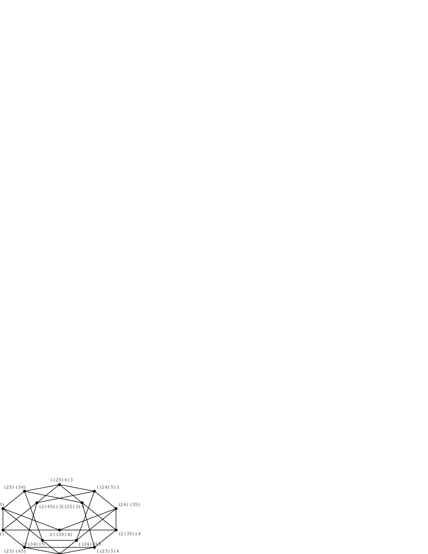
FIG. 2.: The forest of the 15 five-point tree diagrams in unflavored $\phi^{3}$-theory. The diagrams are specified by fixing vertex 1 and using parentheses to denote the order in which lines are joined at vertices.

FIG. 3.: The four-point diagrams $\{t_{4}^{F,1},t_{4}^{F,2},t_{4}^{F,3}\}$ related by flavor flips.

FIG. 4.: The four-point diagrams $\{t_{4}^{G,1},t_{4}^{G,2},t_{4}^{G,3},t_{4}^{G,4}\}$ related by gauge flips.

FIG. 5.: The four-point diagrams $\{t_{4}^{G,5},t_{4}^{G,6},t_{4}^{G,7}\}$ related by gauge flips in the case of fermionic matter.

FIG. 6.: The two ways of adding a matter field pair to a diagram.

FIG. 7.: The forest of size 71 for the process $\gamma\gamma\to u\bar{d}d\bar{u}$ in the standard model (without QCD, CKM mixing and Higgs contributions and in unitarity gauge) with one grove of size 31, two groves of size 12 and two groves of size 8. Solid lines represent gauge flips and dotted lines represent flavor flips.

TABLE I.: The groves for all processes with six external massless fermions and single photon bremsstrahlung in the standard model (without QCD). Six-fermion processes with identical groves can have different groves if a photon is added, because the photon distinguishes leptons from neutrinos in internal lines.

external fields ($E$)	diagrams	classes
$u\bar{u}u\bar{u}u\bar{u}$	$144$	$18\cdot 8$
$u\bar{u}u\bar{u}u\bar{u}\gamma$	$1008$	$18\cdot 24+36\cdot 16$
$u\bar{u}u\bar{u}d\bar{d}$	$92$	$4\cdot 11+6\cdot 8$
$u\bar{u}u\bar{u}d\bar{d}\gamma$	$696$	$4\cdot 90+6\cdot 24+12\cdot 16$
$\ell^{+}\ell^{-}u\bar{u}d\bar{d}$	$27$	$1\cdot 11+2\cdot 8$
$\ell^{+}\ell^{-}u\bar{u}d\bar{d}\gamma$	$201$	$1\cdot 89+2\cdot 24+4\cdot 16$
$\ell^{-}\nu d\bar{u}d\bar{d}$	$20$	$2\cdot 10$
$\ell^{-}\nu d\bar{u}d\bar{d}\gamma$	$142$	$2\cdot 71$
$\ell^{+}\ell^{-}\ell^{-}\nu d\bar{u}$	$20$	$2\cdot 10$
$\ell^{+}\ell^{-}\ell^{-}\nu d\bar{u}\gamma$	$140$	$2\cdot 70$
$\ell^{-}\nu\ell^{+}\bar{\nu}d\bar{d}$	$15$	$1\cdot 9+1\cdot 4+1\cdot 2$
$\ell^{-}\nu\ell^{+}\bar{\nu}d\bar{d}\gamma$	$82$	$1\cdot 54+1\cdot 12+1\cdot 8+2\cdot 4$
$\ell^{-}\bar{\nu}\ell^{+}\nu\ell^{+}\ell^{-}$	$56$	$4\cdot 9+4\cdot 4+2\cdot 2$
$\ell^{-}\bar{\nu}\ell^{+}\nu\ell^{+}\ell^{-}\gamma$	$308$	$4\cdot 53+4\cdot 12+4\cdot 8+4\cdot 4$
$\ell^{+}\nu\ell^{-}\bar{\nu}\nu\bar{\nu}$	$36$	$4\cdot 6+6\cdot 2$
$\ell^{+}\nu\ell^{-}\bar{\nu}\nu\bar{\nu}\gamma$	$120$	$4\cdot 23+2\cdot 6+4\cdot 4$
$\nu\bar{\nu}\nu\bar{\nu}\nu\bar{\nu}$	$36$	$18\cdot 2$

REFERENCES

- [1] D. Bardin et al., Nucl. Phys. (Proc. Suppl.) 37B, 148 (1994).
- [2] E. Boos and T. Ohl, Phys. Lett. B407, 161 (1997).
- [3] E. Boos and T. Ohl, to be published.
- [4] B. D. McKay, Technical. Report TR-CS-90-02, Dept. Comp. Sci., Austral. Nat. Univ. (1990).