The infrared behaviour of the static potential in perturbative QCD

Abstract

The definition of the quark-antiquark static potential is given within an effective field theory framework. The leading infrared divergences of the static singlet potential in perturbation theory are explicitly calculated.
PACS numbers: 12.38.Aw, 12.38.Bx, 12.39.Hg

]

I Introduction

The static singlet potential between a heavy quark and an antiquark is an object of considerable interest both theoretically and phenomenologically. Strictly speaking, being the potential a dynamical quantity, it can be defined only in a context where the full dynamics of the system is consistently taken into account. For instance in the proper Schrödinger equation. Nevertheless, the static singlet potential is usually defined as the logarithm of the static Wilson loop divided by the interaction time in the limit of infinite interaction time. Moreover, the above definition, in QCD, suffers from infrared (IR) divergences when computed at finite orders of perturbation theory [1]. This has to do with the non-Abelian nature of QCD, which allows massless gluons to self-interact at arbitrarily small energy scales.

The problem was posed in the past [1] of whether the static singlet potential could be defined in some way at any order in perturbation theory. The leading IR singularities in the static Wilson loop were found at a relative order $\alpha_{\rm s}^{3}$ in [1]. These singularities can indeed be regulated upon resummation of a certain class of diagrams which give rise to a dynamical cut-off provided by the difference between the singlet and the octet potentials. However, the extraction of the static singlet quark-antiquark ($Q$-$\bar{Q}$) potential from this resummation has been regarded as suspect by other authors [2], who noticed that the difference between the singlet and the octet potential provides a dynamical scale which, at least in perturbation theory, is of the same order of the kinetic energy for quarks of large but finite mass. A similar situation occurs in QED for the Lamb shift, where one of the contributions has to be interpreted as a non-potential correction to the hydrogen atom energy levels. The novel feature in QCD is that such an effect appears to be related to the definition of the static potential, while in QED it is of order $1/m^{2}$. No quantitative procedure has been developed so far to deal with this problem in QCD.

The recent complete calculation of the static potential at two loops [3] and its foreseen applications to top pair production at the Next Linear Collider [4] brings this problem to the edge of experimentally testable physics. We feel that a clear resolution is urgently needed.

It is the aim of this paper to fully clarify this problem by providing a quantitative framework where the different scales that characterize a non-relativistic system can be properly taken into account. This is achieved by using an effective field theory approach.

We will assume that $mv\gg\Lambda_{\rm QCD}$, $m$ and $v$ being the heavy-quark mass and velocity respectively ($v\ll 1$). Then we will systematically integrate out the hard ($\sim m$) and soft ($\sim mv$) degrees of freedom by performing in both cases a perturbative matching to suitable effective field theories. The integration of the hard scale gives rise to non-relativistic QCD (NRQCD) [5], whereas the integration of the soft scale gives rise to potential NRQCD (pNRQCD) [6]. In the latter effective theory only ultrasoft (US) degrees of freedom are left, which in this letter means the ones with energy much smaller than $mv$. The static potential can be understood as a matching coefficient in pNRQCD.

The main result of this work is to state rigorously what in perturbative QCD has to be understood as the $Q$-$\bar{Q}$ static potential, namely the relevant object for the dynamics of $Q$-$\bar{Q}$ pairs with large but finite mass. This does not simply coincide with the static Wilson loop as usually computed, since this turns out to contain US contributions as well. As a consequence the static potential manifests, at the relative order $\alpha_{\rm s}^{3}$, an explicit dependence on the cut-off of the effective theory and has to be understood as a matching coefficient in pNRQCD. The leading cut-off dependence is evaluated explicitly.

II Theoretical Framework

After integrating out the hard scale ($\sim m$) from QCD, we are left with NRQCD. For our purposes it is sufficient to work at the lowest order in the NRQCD Lagrangian, namely,

$${\cal L}_{\rm NRQCD}\! = \!\psi^{\dagger}\!\left\{iD^{0}+{{\bf D}^{2}\over 2m}\right\}\!\psi+\chi^{\dagger}\!\left\{iD^{0}-{{\bf D}^{2}\over 2m}\right\}\!\chi$$ (2)

$$-{1\over 4}F_{\mu\nu}^{a}F^{\mu\nu\,a}\,,$$

where $\psi$ is the Pauli spinor field that annihilates the fermion and $\chi$ is the Pauli spinor field that creates the antifermion; $iD^{0}=i\partial_{0}-gA^{0}$ and $i{\bf D}=i{\mbox{\boldmath$\nabla$}}+g{\bf A}$.

Integrating out also the soft scale, $mv$, from (2) we are left with an effective theory (pNRQCD) where only US degrees of freedom remain dynamical. The surviving fields are the $Q$-$\bar{Q}$ states (with US energy) and the US gluons. The $Q$-$\bar{Q}$ states can be decomposed into a singlet (S) and an octet (O) under colour transformation. The relative coordinate ${\bf r}={\bf x}_{1}-{\bf x}_{2}$, whose typical size is the inverse of the soft scale, is explicit and can be considered as small with respect to the remaining (US) dynamical lengths in the system. Hence the gluon fields can be systematically expanded in $\bf r$ (multipole expansion). Therefore the pNRQCD Lagrangian is constructed not only order by order in $1/m$, but also order by order in ${\bf r}$. As a typical feature of an effective theory, all the non-analytic behaviour in ${\bf r}$ is encoded in the matching coefficients, which can be interpreted as potential-like terms.

The most general pNRQCD Lagrangian density that can be constructed with these fields and that is compatible with the symmetries of NRQCD is given at the leading order in the multipole expansion by:

$${\cal L}_{\rm pNRQCD}={\rm Tr}\Biggl{\{}{\rm S}^{\dagger}\left(i\partial_{0}-{{\bf p}^{2}\over m}-V_{s}(r)+\dots\right){\rm S}$$ (3)

$$\qquad+{\rm O}^{\dagger}\left(iD_{0}-{{\bf p}^{2}\over m}-V_{o}(r)+\dots\right){\rm O}\Biggr{\}}$$ (4)

$$\qquad+gV_{A}(r){\rm Tr}\left\{{\rm O}^{\dagger}{\bf r}\cdot{\bf E}\,{\rm S}+{\rm S}^{\dagger}{\bf r}\cdot{\bf E}\,{\rm O}\right\}$$ (5)

$$\qquad+g{V_{B}(r)\over 2}{\rm Tr}\left\{{\rm O}^{\dagger}{\bf r}\cdot{\bf E}\,{\rm O}+{\rm O}^{\dagger}{\rm O}{\bf r}\cdot{\bf E}\right\},$$ (6)

where ${\bf R}\equiv({\bf x}_{1}+{\bf x}_{2})/2$, ${\rm S}={\rm S}({\bf r},{\bf R},t)$ and ${\rm O}={\rm O}({\bf r},{\bf R},t)$ are the singlet and octet wave functions respectively. All the gauge fields in Eq. (6) are evaluated in ${\bf R}$ and $t$. In particular ${\bf E}\equiv{\bf E}({\bf R},t)$ and $iD_{0}{\rm O}\equiv i\partial_{0}{\rm O}-g[A_{0}({\bf R},t),{\rm O}]$. $V_{s}$ and $V_{o}$ are the singlet and octet heavy $Q$-$\bar{Q}$ static potential respectively. Higher-order potentials in the $1/m$ expansion and the centre-of-mass kinetic terms are irrelevant here and are neglected. We define

$$V_{s}(r) \equiv -C_{F}{\alpha_{V_{s}}(r)\over r},$$ (7)

$$V_{o}(r) \equiv \left({C_{A}\over 2}-C_{F}\right){\alpha_{V_{o}}(r)\over r}.$$ (8)

$V_{A}$ and $V_{B}$ are the matching coefficients associated in the Lagrangian (6) to the leading corrections in the multipole expansion. Both the potentials and the coefficients $V_{A}$ and $V_{B}$ have to be determined by matching pNRQCD with NRQCD at a scale $\mu$ smaller than $mv$ and larger than the US scales. Since, in particular, $\mu$ is larger than $\Lambda_{\rm QCD}$ the matching can be done perturbatively. At the lowest order in the coupling constant we get $\alpha_{V_{s}}=\alpha_{V_{o}}=\alpha_{\rm s}$, $V_{A}=V_{B}=1$. In order to have the proper free-field normalization in the colour space we define

$${\rm S}\equiv{1\!\!{\rm l}_{c}\over\sqrt{N_{c}}}S\quad\quad{\rm O}\equiv{T^{a}\over\sqrt{T_{F}}}O^{a},$$ (9)

where $T_{F}=1/2$.

III Matching

In this section we discuss how to perform the matching between NRQCD and pNRQCD. In particular we will concentrate on the effects produced by the leading corrections coming from the multipole expansion.

The matching is in general done by comparing 2-fermion Green functions (plus external gluons at the ultrasoft scale) in NRQCD and pNRQCD, order by order in $1/m$ and order by order in the multipole expansion. If the soft scale is in the perturbative region of QCD (i.e. larger than $\Lambda_{\rm QCD}$), this can be done explicitly order by order in the coupling constant. If not, one can still perform the matching by subtracting the calculation in pNRQCD to the desired order of accuracy. The remaining term only contains the soft scale (up to US higher-order corrections) and goes in the pNRQCD Lagrangian as a new potential term.

The matching can be done once the interpolating fields for $S$ and $O^{a}$ have been identified in NRQCD. The former need to have the same quantum numbers and the same transformation properties as the latter. We choose the following definitions for the singlet

$$\chi^{\dagger}({\bf x}_{2},t)\phi({\bf x}_{2},{\bf x}_{1},t)\psi({\bf x}_{1},t)=Z^{1/2}_{s}(r)S({\bf R},{\bf r},t)$$

and for the octet

$$\!\!\!\chi^{\dagger}({\bf x}_{2},t)\phi({\bf x}_{2},{\bf R},t)T^{a}\phi({\bf R},{\bf x}_{1},t)\psi({\bf x}_{1},t)$$

$$\qquad\quad=Z^{1/2}_{o}(r)O^{a}({\bf R},{\bf r},t),$$

where

$$\phi({\bf y},{\bf x},t)\equiv{\rm P}\exp\Big{\{}\!ig\displaystyle\int_{0}^{1}\!\!ds\,({\bf y}-{\bf x})\cdot{\bf A}({\bf x}-s({\bf x}-{\bf y}),t)\!\Big{\}}.$$

From the normalization condition (9) it follows, at the tree level, that $Z_{s}=N_{c}$ and $Z_{o}=T_{F}$.

In order to get the singlet potential, we choose the following Green function:

$$I \equiv \langle 0|\chi^{\dagger}(x_{2})\phi(x_{2},x_{1})\psi(x_{1})$$ (11)

$$\qquad\times\psi^{\dagger}(y_{1})\phi(y_{1},y_{2})\chi(y_{2})|0\rangle.$$

In NRQCD we obtain, at order $(1/m)^{0}$:

$$I=\delta^{3}({\bf x}_{1}-{\bf y}_{1})\delta^{3}({\bf x}_{2}-{\bf y}_{2})\langle W_{\Box}\rangle,$$ (12)

where $W_{\Box}$ is the rectangular Wilson loop with edges $x_{1}=(T/2,{\bf r}/2)$, $x_{2}=(T/2,-{\bf r}/2)$, $y_{1}=(-T/2,{\bf r}/2)$ and $y_{2}=(-T/2,-{\bf r}/2)$. The symbol $\langle~{}~{}\rangle$ means the average over the gauge fields.

b

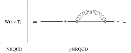
FIG. 1.: The matching of the static potential. On the right side are the pNRQCD fields: simple lines are singlet propagator, double lines are octet propagators, circled-crosses are the singlet-octet vertices of Eq. (6) and the wavy line is the US gluon propagator.

In pNRQCD we obtain at order $(1/m)^{0}$ and at the next-to-leading order in the multipole expansion

$$I=Z_{s}(r)\delta^{3}({\bf x}_{1}-{\bf y}_{1})\delta^{3}({\bf x}_{2}-{\bf y}_{2})e^{-iTV_{s}(r)}$$ (13)

$$\times\Biggl{(}1-{g^{2}\over N_{c}}V_{A}^{2}(r)\int_{-T/2}^{T/2}\!\!dt\int_{-T/2}^{t}\!\!dt^{\prime}e^{-i(t-t^{\prime})(V_{o}-V_{s})}$$ (14)

$$\quad\times\langle{\rm Tr}\{{\bf r}\cdot{\bf E}(t)\phi(t,t^{\prime}){\bf r}\cdot{\bf E}(t^{\prime})\phi(t^{\prime},t)\}\rangle\Biggr{)}.$$ (15)

Fields with only temporal argument are evaluated in the centre-of-mass coordinate.

Comparing Eqs. (12) and (15), one gets at the next-to-leading order in the multipole expansion the singlet wave-function normalization $Z_{s}$ and the singlet static potential $V_{s}$ (see Fig. 1). $V_{A}(r)$ and $V_{o}(r)$ must have been previously obtained from the matching of suitable operators. Since here we shall only need the tree-level results, we postpone the general discussion to [7]. We shall further concentrate on the singlet potential while the wave function normalization will also be discussed in [7]. The explicit calculation can be done in several (equivalent) ways:

i) By matching order by order in $\alpha_{\rm s}$ [7]. Both expressions (12) and (15) are IR-divergent (Eq. (15) is also UV-divergent). Regulating both expressions in dimensional regularization the calculation in pNRQCD gives zero (there is no scale), while the calculation of the Wilson loop shows up an explicit dependence on the infrared regulator $\mu$ via a typical $\ln\mu r$ term.

ii) By keeping, without expanding, in (15) the exponentials in $V_{o}$ and $V_{s}$. The scale $V_{o}-V_{s}$, which appears in this way, regulates the IR divergences in Eq. (15). Because of this scale, the calculation in pNRQCD now gives a non-zero contribution proportional to the UV cut-off $\mu$ of the theory ($\sim\ln(V_{o}-V_{s})/\mu$). This calculation would be sufficient to extract the leading IR divergences of the static potential, in the same way as it is sufficient to evaluate the leading logarithm in the effective field theory in order to know the running of a matching coefficient. However, in order to carry out the matching consistently, we have to evaluate (12) in a way that exactly corresponds to keeping the exponentials in (15). For the IR-singular terms in NRQCD, this way is nothing but the resummation of the diagrams depicted in Fig. 2, as it was indicated in [1]. This procedure is automatically adopted in any attempt to extract the (non-perturbative) static potential from a non-perturbative evaluation of the Wilson loop (e.g. in lattice calculations).

b

FIG. 2.: Graphs contributing to $\delta\langle W_{\Box}\rangle$. Dashed lines represent Coulomb exchanges.

In order to make the comparison with [1] easier, we will follow here this second approach. We will show the cancellation of the $\ln(V_{o}-V_{s})$ terms explicitly. Evaluating expressions (12) and (15) with the prescription ii) we get, for the static potential at the next-to-leading order in the multipole expansion:

$$V_{s}(r;\mu)=\lim_{T\rightarrow\infty}{i\over T}\ln{\langle W_{\Box}\rangle}$$ (16)

$$+C_{F}{\alpha_{\rm s}\over\pi}{r^{2}\over 3}(V_{o}-V_{s})^{3}\ln{(V_{o}-V_{s})^{2}\over 4\pi\mu^{2}}.$$ (17)

The dependence on $\ln(V_{o}-V_{s})$ in the second line is canceled in the first line by the contribution to the Wilson loop ($\delta\langle W_{\Box}\rangle$) coming from the graphs shown in Fig. 2 whose qualitative features were considered in [1, 8]. Indeed, the exact calculation done in this work gives

$$\lim_{T\rightarrow\infty}{i\over T}\ln{\delta\langle W_{\Box}\rangle} = -C_{F}C_{A}^{2}{\alpha_{\rm s}^{3}\over 12\pi}(V_{o}-V_{s})$$ (19)

$$\qquad\quad\times\ln\left({(V_{o}-V_{s})^{2}r^{2}}\right).$$

Finally, the result given in Eq. (17) allows us to write the complete expression for the static potential, Eq. (7), up to the relative order $\alpha_{\rm s}^{3}\ln\mu r$ in coordinate space ($\alpha_{\rm s}$ is in the $\overline{\rm MS}$ scheme):

$${\alpha}_{V_{s}}(r,\mu)=\alpha_{\rm s}(r)\left\{1+\left(a_{1}+2{\gamma_{E}\beta_{0}}\right){\alpha_{\rm s}(r)\over 4\pi}\right.$$ (20)

$$+\left[\gamma_{E}\left(4a_{1}\beta_{0}+2{\beta_{1}}\right)+\left({\pi^{2}\over 3}+4\gamma_{E}^{2}\right){\beta_{0}^{2}}+a_{2}\right]{\alpha_{\rm s}^{2}(r)\over 16\,\pi^{2}}$$ (21)

$$\left.+{C_{A}^{3}\over 12}{\alpha_{\rm s}^{3}(r)\over\pi}\ln{r\mu}\right\},$$ (22)

where $\beta_{n}$ are the coefficients of the beta function, $a_{1}$ was calculated in Ref. [9] and $a_{2}$ in Ref. [3] (see [3] for notation). We emphasize that this new contribution to the static potential would be zero in QED.

IV Conclusions

Eq. (22) is the main result of this letter. It states that $\alpha_{V_{s}}$, defined through the static potential (see Eq. (7)), is not a short distance quantity as $\alpha_{\rm s}$ (in the ${\rm\overline{MS}}$ scheme), since it depends on the IR behaviour of the theory. It can be better understood as a matching coefficient (an analogous situation occurs for the pole mass). Moreover Eq. (22) gives the analytic value of the coefficient of the leading $\ln\mu r$ correction, which arises at relative order $\alpha_{\rm s}^{3}$, i.e. immediately after the known two-loop corrections. The situation for the static octet potential seems to be similar [7].

The evaluated terms clarify the long-standing issue of how the perturbative static potential should be defined at higher order in the perturbative series. Eq. (17) explicitly shows that the static potential does not coincide with the static Wilson loop as usually computed. It should be emphasized that the separation between soft and US contributions is not an artificial trick but a necessary procedure if one wants to use the static potential in a Schrödinger-like equation in order to study the dynamics of $Q$-$\bar{Q}$ states of large but finite mass. In that equation the kinetic term of the $Q$-$\bar{Q}$ system is US and so is the energy. Since the US gluons interact with the $Q$-$\bar{Q}$ system, their dynamics is sensitive to the energies of the (non-static) system and hence it is not correct to include them in the static potential. When calculating a physical observable the $\mu$ dependence in (10) must cancel against $\mu$-dependent contributions coming from the US gluons.

Finally it is worth mentioning that the static potential suffers from IR renormalons ambiguities with the following structure

$$\delta V_{s}\sim C+C_{2}r^{2}+.\,.\,.$$

The constant $C$ is known to be cancelled by the IR pole mass renormalon [10] while the IR $C_{2}$ renormalon gets cancelled by the IR renormalon existing in the second term of Eq. (15) [7].

N.B. acknowledges the TMR contract No. ERBFMBICT961714, A.P. the TMR contract No. ERBFMBICT983405, J.S. the AEN98-031 (Spain) and 1998SGR 00026 (Catalonia) and A.V. the FWF contract No. 9013.

REFERENCES

- [1] T. Appelquist, M. Dine and I. J. Muzinich, Phys. Rev. D 17, 2074 (1978).
- [2] L. S. Brown and W.I. Weisberger, Phys. Rev. D 20, 3239 (1979); B. A. Thacker and G. P. Lepage, Phys. Rev. D 43, 196 (1991).
- [3] Y. Schröder, Phys. Lett. B 447, 321 (1999); M. Peter, Phys. Rev. Lett. 78, 602 (1997).
- [4] M. Beneke, A. Signer and V.A. Smirnov, hep-ph/9903260; A. Hoang, hep-ph/9809431.
- [5] W. E. Caswell and G. P. Lepage, Phys. Lett. B 167, 437 (1986); G.T. Bodwin, E. Braaten and G.P. Lepage, Phys. Rev. D 51, 1125 (1995), Erratum ibid. D55, 5853 (1997).
- [6] A. Pineda and J. Soto, Nucl. Phys. B (Proc. Suppl.) 64, 428 (1998).
- [7] N. Brambilla, A. Pineda, J. Soto and A. Vairo, in preparation.
- [8] W. Kummer, W. Mödritsch and A. Vairo, Z. Phys. C 72, 653 (1996).
- [9] A. Billoire, Phys. Lett. B 92, 343 (1980).
- [10] A. Pineda, PhD thesis, Univ. Barcelona (1998).