hep-ph/9903354 VUTH 99-03 Time-reversal odd fragmentation and distribution functions
in pp and ep single spin asymmetries.

Abstract

We present some estimates of T-odd fragmentation and distribution functions, $H_{1}^{\perp}$ and $f_{1T}^{\perp}$, evaluated on the basis of a fit on experimental data in p^↑p. Assuming the T-odd fragmentation function to be responsible for the single spin asymmetry in pion production in p^↑p, we find the ratio $H_{1}^{\perp}/D_{1}$ to be in good agreement with the experimental results from DELPHI data on $Z\,\to\,2$-jet decay. We use our estimates to make predictions for ep^↑.

I Introduction

High energy scattering processes, e.g. unpolarized and polarized deep inelastic scattering, provide an efficient tool to investigate the internal structure of nucleons. Particularly interesting is the study of the role that elementary constituents play in accounting for the total spin of the proton: a joint theoretical and experimental effort is required to gain complete knowledge and understanding of quark and gluon contributions to the spin structure of hadrons, in high energy processes.

At leading order in $1/Q$, the cross section for a hard process $a+b\to c+d$ is given by the convolution of a ‘hard part’, which describes the scattering among elementary constituents and can be calculated perturbatively in the framework of QCD, and a ‘soft’ part, that accounts for the processes in which either quarks are produced from the initial hadrons or final hadrons are produced from quarks resulting from the hard elementary scattering. Distribution functions belong to the first class of soft parts whereas fragmentation functions belong to the second class.

The most well-known distribution function, which we will indicate by $f^{a}_{1}(x)$, is the number density of quarks with flavour $a$ carrying a momentum fraction $x$ in an unpolarized proton; analogously, the fragmentation function $D_{1}^{a}(z_{h})$ gives the density number of hadrons $h$ with momentum fraction $z_{h}$, resulting from the fragmentation of a quark of flavour $a$. When we consider polarized processes the number of distribution and fragmentation functions increases considerably. More specifically, we take into account the possibility of either extracting unpolarized quarks from polarized hadrons, or creating unpolarized or spinless hadrons from polarized quarks.

To distinguish among the various processes, we employ the following conventions (first introduced in Ref. [1] and later generalized in Ref. [2]):

• $f$ and $D$ apply to non polarized quarks in the proton or in the hadron respectively;

• $g$ and $G$ apply to longitudinally polarized quarks;

• $h$ and $H$ apply to transversely polarized quarks;

• the subscripts $L$ and $T$ refer to the longitudinal and transverse polarization of the target or produced (spin 1/2) hadron;

• A subscript $1$ indicates “leading order” (we will not deal with subleading functions here).

• In several polarized distribution and fragmentation functions, the intrinsic transverse momenta of quarks play an important role. In that case a superscript ${\perp}$ is used to signal such a dependence on $\mbox{\boldmath$k$}_{\scriptscriptstyle T}$, while a superscript $(1)$ indicates that a function is integrated over $\mbox{\boldmath$k$}_{\scriptscriptstyle T}$, after a weighting with $\mbox{\boldmath$k$}_{\scriptscriptstyle T}^{2}/2M^{2}$, see for example Eqs. (32,55).

Figs 1 and 2 give a pictorial representation of these functions, and illustrate how the principles stated above are applied. The distribution function $f_{1}^{a}$ is the probability of finding an unpolarized quark $a$ into an unpolarized proton; this is a very well known object, usually determined by fits on unpolarized DIS experimental data. The distribution functions $g_{1L}^{a}$ and $g_{1T}^{a}$ are proportional to the probability of finding a quark with longitudinal polarization either in a longitudinally or in a transversely polarized proton, whereas $h_{1T}^{a}$ is proportional to the probability to find a transversely polarized quark $a$ in a transversely polarized hadron. In a completely analogous way, the fragmentation function $D_{1}^{a}$ is the probability of an unpolarized quark $a$ to fragment into an unpolarized hadron, whereas $G_{1L}^{a}$, $G_{1T}^{a}$, $H_{1T}^{a}$ take into account the probability of either longitudinally or transversely polarized quarks fragmenting into longitudinally or transversely polarized hadrons respectively. In addition, we have distribution and fragmentation functions which are directly proportional to the intrinsic transverse momentum of the quarks inside the hadron; their contribution would then be zero in the approximation of zero intrinsic momentum. As shown in Figs. 1 and 2, $h_{1L}^{\perp a}$ and $h_{1T}^{\perp a}$ give the probability of a transversely polarized quark $a$ to be found in a longitudinaly or transversely polarized proton. Similarly, for fragmentation functions, we have $H_{1L}^{\perp}$ and $H_{1T}^{\perp}$.

The distribution functions $f_{1T}^{\perp a}(x)$ and $h_{1}^{\perp a}(x)$, and the analogous fragmentation functions $D_{1T}^{\perp}(z)$ and $H_{1}^{\perp}(z)$ are particularly “delicate” and controversial objects. In fact, as it was extensively discussed in Ref. [3], those are T-odd functions (i.e. they are not constrained by time reversal invariance). This non-applicability of time reversal symmetry is straightforwardly understood in the case of fragmentation functions, since the produced hadron can interact with the remnants of the fragmenting quark [4]. Thus, a non-zero $H_{1}^{\perp}(z)$ allows for processes in which transversely polarized quarks fragment into unpolarized hadron (see picture in Fig. 2). Notice that, as it was pointed out in Refs. [5] and [6] a more accurate knowledge of this functions would give a unique chance to do spin physics with unpolarized or spin zero hadrons.

In the case of the distribution functions, the non-application of time reversal symmetry can still be accepted, due to soft initial state interactions [7] (it is, in fact, reasonable to believe that, in processes in which two hadrons are in the initial state, debris from the “distribution” process may soft-interact, mutually and with the quark which will be involved in the hard scattering) or, possibly, as a consequence of chiral symmetry breaking, as suggested in Ref. [8]. Furthermore, they can also arise effectively from higher order processes where soft gluons may produce so-called gluonic poles [9] . All in all, the $f_{1T}^{\perp a}(x)$ function being non-zero allows for processes in which unpolarized quarks are produced from a polarized proton (see picture in Fig. 1).

But what about the real world? Are these effects really detectable in experiments? And what is the size of the effects generated by them? Investigating the $f_{1T}^{\perp a}(x)$ and $H_{1}^{\perp a}(z)$ is what this paper is about.

For our estimates, we will benefit from two essential inputs: first of all we will use the parametrizations presented in Ref. [7] (or better those given in the revamped version of Ref. [10]) and in Ref. [11]. In the first references, Anselmino et al. find an explicit parametrization for the $f_{1T}^{\perp a}(x)$ by fitting the data on single spin asymmetry in $p^{\uparrow}\,p\,\to\,\pi\,X$ from FNAL E704 experiment [12], assuming the presence of Sivers effect only [13], i.e. taking into account $k_{\perp}$ effects in the polarized proton initial state only. In Ref. [11] the same authors present a parametrization of the $H_{1}^{\perp}(z)$ fragmentation function, based on a fit on the same experimental data, but taking into account only the Collins effect [14], thus assuming that the quark intrinsic transverse momentum has a relevant role in the final pion state kinematics only (see discussion in Ref. [11] for more details).
The second input we use is from Ref. [3], where the authors explain how the T-odd fragmentation and distribution functions can be incorporated in their formalism and suggest the use of some weighted integrals to get more information about them from measurements of specific angles ($\phi^{l}_{h}$ and $\phi^{l}_{S}$ in this particular case, which are the angle between the lepton scattering plane and the produced hadron plane, and the angle between the lepton scattering plane and the nucleon spin, respectively).

In Section II we give a description of the formalism and notations and we analyze the relations between the correlators in the spin and helicity basis. We then discuss the connections between the distribution and fragmentation functions evaluated in Refs. [7, 10, 11] and those presented in Ref. [3]. In Section III the shape of some weighted integrals is shown as a function of $x$ and $z_{h}$ in tri-dimensional plots; they illustrate how time-reversal odd functions appear in some experimentally accessible observables. In the last Section we estimate the ratios $H_{1}^{\perp}/D_{1}$ and $f_{1T}^{\perp}/f_{1}$ and compare them with existing experimental data. In the concluding paragraph we will discuss the future perspectives and the experimental work that we recommend for a better and deeper understanding of these functions, and the interesting physics still hidden inside them.

II Quark correlation functions

A Definitions for distribution functions

 

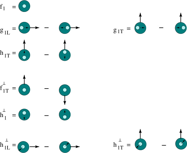
FIG. 1.: Pictorial representation of the various kinds of distribution functions

 

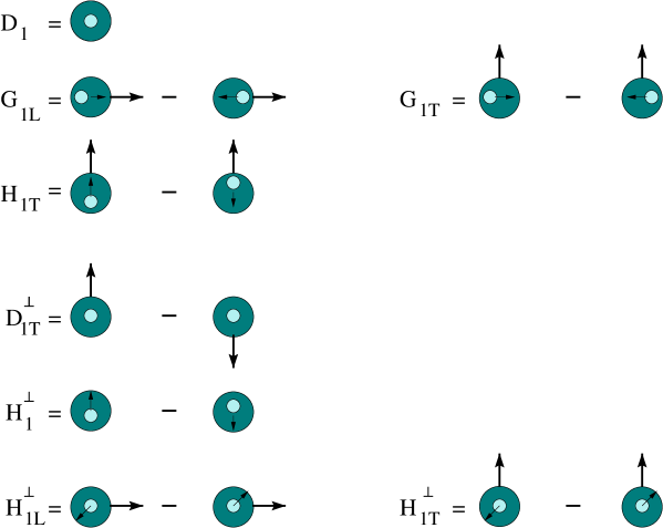
FIG. 2.: Pictorial representation of the various kinds of fragmentation functions

The quark distribution functions alluded to in the introduction appear in the parametrization of the lightfront correlation function [15]

$$\Phi_{ij}(x,\mbox{\boldmath$k$}_{\scriptscriptstyle T};P,S)=\frac{1}{2}\,\left.\int\frac{d\xi^{-}d^{2}\mbox{\boldmath$\xi$}_{\scriptscriptstyle T}}{(2\pi)^{3}}\ e^{ik\cdot\xi}\,\langle P,S|\overline{\psi}_{j}(0)\psi_{i}(\xi)|P,S\rangle\right|_{\xi^{+}=0},$$ (1)

which depends on the lightcone fraction of the quark momentum, $x=k^{+}/P^{+}$ and the transverse momentum component $\mbox{\boldmath$k$}_{\scriptscriptstyle T}$. For this purpose we use lightlike vectors $n_{\pm}$, satisfying $n_{+}\cdot n_{-}=1$ and defining the lightcone coordinates $a^{\pm}$ = $a\cdot n_{\mp}$. The lightlike vectors are defined by the hadron momentum, $P$ $\equiv$ $P^{+}n_{+}+(M^{2}/2P^{+})n_{-}$, where $n_{-}$ is defined via another vector in the hard scattering process, e.g. the momentum transfer $q$ in inclusive deep inelastic scattering or the ‘other’ hadron momentum in pp scattering. The definitions of $x$ and $\mbox{\boldmath$k$}_{\scriptscriptstyle T}$ are contained in $k$ $\equiv$ $x\,P^{+}n_{+}+k^{-}n_{-}+k_{\scriptscriptstyle T}$.

Using Lorentz invariance, hermiticity, and parity invariance one finds that the Dirac structure relevant in a calculation up to leading order in $1/Q$ is given by [3]

$$\Phi(x,\mbox{\boldmath$k$}_{\scriptscriptstyle T};P,S) = \frac{1}{4}\Biggl{\{}f_{1}\,\hbox to0.0pt{/\hss}\hbox to0.0pt{/\hss}n_{+}+f_{1T}^{\perp}\,\frac{\epsilon_{\mu\nu\rho\sigma}\gamma^{\mu}n_{+}^{\nu}k_{\scriptscriptstyle T}^{\rho}S_{\scriptscriptstyle T}^{\sigma}}{M}+g_{1s}\,\gamma_{5}\hbox to0.0pt{/\hss}n_{+}$$ (3)

$$\qquad+h_{1T}\,i\sigma_{\mu\nu}\gamma_{5}n_{+}^{\mu}S_{\scriptscriptstyle T}^{\nu}+h_{1s}^{\perp}\,\frac{i\sigma_{\mu\nu}\gamma_{5}n_{+}^{\mu}k_{\scriptscriptstyle T}^{\nu}}{M}+h_{1}^{\perp}\,\frac{\sigma_{\mu\nu}k_{\scriptscriptstyle T}^{\mu}n_{+}^{\nu}}{M}\Biggr{\}},$$

with arguments $f_{1}$ = $f_{1}(x,\mbox{\boldmath$k$}_{\scriptscriptstyle T}^{2})$ etc. Note that the factor $1/2$ in Eq. (1) and the parametrization of Eq. (3) are chosen to get the proper normalization of the distribution functions, $\int dx\ d^{2}\mbox{\boldmath$k$}_{\scriptscriptstyle T}\ f_{1}^{a}(x,\mbox{\boldmath$k$}_{\scriptscriptstyle T})=n_{a}$, from the relation $\langle P,S|\overline{\psi}(0)\gamma^{+}\psi(0)|P,S\rangle$ = $2P^{+}\,n_{a}$. The quantity $g_{1s}$ (and similarly $h_{1s}^{\perp}$) is shorthand for

$$g_{1s}(x,\mbox{\boldmath$k$}_{\scriptscriptstyle T})=\lambda\,g_{1L}(x,\mbox{\boldmath$k$}_{\scriptscriptstyle T}^{2})+\frac{\mbox{\boldmath$k$}_{\scriptscriptstyle T}\cdot\mbox{\boldmath$S$}_{\scriptscriptstyle T}}{M}\,g_{1T}(x,\mbox{\boldmath$k$}_{\scriptscriptstyle T}^{2}),$$ (4)

with $M$ the mass, $\lambda=M\,S^{+}/P^{+}$ the lightcone helicity, and $\mbox{\boldmath$S$}_{\scriptscriptstyle T}$ the transverse spin of the target hadron. In fact, we have $S$ $\equiv$ $\lambda\,(P^{+}/M)\,n_{+}-\lambda\,(M/2P^{+})\,n_{-}+S_{\scriptscriptstyle T}$ and thus in the the restframe $S=(0,\mbox{\boldmath$S$}_{\scriptscriptstyle T},\lambda)$. The lightcone helicity, thus, is a convenient quantity which in the target rest frame is just the third component of the spin vector, while in the infinite momentum frame ($P^{+}\rightarrow\infty$) it is proportional to the standard helicity.

B Correlators in helicity basis

In order to compare with other results we give the link with the helicity formalism, used in Refs. [7, 11]. This is achieved by transforming the $\Phi_{ij}$ matrix elements to the helicity basis with the help of the density matrix $\rho$, in the target rest frame given by

$$\rho_{\Lambda\Lambda^{\prime}}=\frac{1}{2}\;(\delta_{\Lambda\Lambda^{\prime}}+\mbox{\boldmath$S$}\cdot(\mbox{\boldmath$\sigma$})_{\Lambda\Lambda^{\prime}})\;,$$ (5)

where $\Lambda$, $\Lambda^{\prime}$ are the helicity indices of the proton and $S$ the spin vector used in the above expression. In fact the parametrization using the spin vector $S$ is defined as

$$\Phi_{ij}(x,k_{\scriptscriptstyle T};P,S)=\sum_{\Lambda\Lambda^{\prime}}\rho_{\Lambda\Lambda^{\prime}}(S)\;\Phi_{\Lambda i;\,\Lambda^{\prime}j}(x,k_{\scriptscriptstyle T};P).$$ (6)

Using the restframe result $S=(0,\mbox{\boldmath$S$}_{\scriptscriptstyle T},\lambda)$ one obtains

$$\Phi_{ij}(x,\mbox{\boldmath$k$}_{\scriptscriptstyle T},P,S) = \frac{1}{2}\Bigl{(}\Phi_{+i;\,+j}+\Phi_{-i;\,-j}\Bigr{)}+\frac{1}{2}\,\lambda\Bigl{(}\Phi_{+i;\,+j}-\Phi_{-i;\,-j}\Bigr{)}$$ (8)

$$\mbox{}+\frac{1}{2}\,S_{\scriptscriptstyle T}^{1}\Bigl{(}\Phi_{+i;\,-j}+\Phi_{-i;\,+j}\Bigr{)}-\frac{i}{2}\,S_{\scriptscriptstyle T}^{2}\Bigl{(}\Phi_{+i;\,-j}-\Phi_{-i;\,+j}\Bigr{)},$$

where one could have used transverse spin differences instead of the off-diagonal helicity matrix elements. One immediately sees that

$$\Bigl{(}\Phi_{+i;\,-j}+\Phi_{-i;\,+j}\Bigr{)}=\Bigl{(}\Phi_{\uparrow_{x}i;\,\uparrow_{x}j}-\Phi_{\downarrow_{x}i;\,\downarrow_{x}j}\Bigr{)},$$ (9)

$$-i\,\Bigl{(}\Phi_{+i;\,-j}-\Phi_{-i;\,+j}\Bigr{)}=\Bigl{(}\Phi_{\uparrow_{y}i;\,\uparrow_{y}j}-\Phi_{\downarrow_{y}i;\,\downarrow_{y}j}\Bigr{)}.$$ (10)

The Dirac structure of the above matrix elements can be translated into quark chiralities (for massless quarks, helicities) or transverse spin, by using the appropriate Dirac projection operators, $P_{R/L}=(1\pm\gamma_{5})/2$ or $P_{\uparrow_{i}/\downarrow_{i}}$ $=(1\pm\gamma^{i}\gamma_{5})/2$ respectively, in combination with the projector onto the so-called good components, $P_{+}=\gamma^{-}\gamma^{+}/2$. Explicitly, for $\Phi_{ij}$ we can relate specific projections $\mbox{Tr}\left(\Phi\,\Gamma\right)$ to transverse spin matrix elements or off-diagonal quark chirality matrix elements $\Phi_{\lambda\lambda^{\prime}}$ (see Ref. [1]),

$$\Phi^{[\gamma^{+}]}(x,\mbox{\boldmath$k$}_{\scriptscriptstyle T};P,S)=\mbox{Tr}\,\Bigl{(}\Phi\,\gamma^{+}\Bigr{)}\equiv\Phi_{RR}+\Phi_{LL},$$ (11)

$$\Phi^{[\gamma^{+}\gamma_{5}]}(x,\mbox{\boldmath$k$}_{\scriptscriptstyle T};P,S)=\mbox{Tr}\,\Bigl{(}\Phi\,\gamma^{+}\gamma_{5}\Bigr{)}\equiv\Phi_{RR}-\Phi_{LL},$$ (12)

$$\Phi^{[i\sigma^{1+}\gamma_{5}]}(x,\mbox{\boldmath$k$}_{\scriptscriptstyle T};P,S)=\mbox{Tr}\,\Bigl{(}\Phi\,i\sigma^{1+}\gamma_{5}\Bigr{)}\equiv\Phi_{\uparrow_{x}\uparrow_{x}}-\Phi_{\downarrow_{x}\downarrow_{x}}=\Phi_{RL}+\Phi_{LR},$$ (13)

$$\Phi^{[i\sigma^{2+}\gamma_{5}]}(x,\mbox{\boldmath$k$}_{\scriptscriptstyle T};P,S)=\mbox{Tr}\,\Bigl{(}\Phi\,i\sigma^{2+}\gamma_{5}\Bigr{)}\equiv\Phi_{\uparrow_{y}\uparrow_{y}}-\Phi_{\downarrow_{y}\downarrow_{y}}=-i\Bigl{(}\Phi_{RL}-\Phi_{LR}\Bigr{)}.$$ (14)

The Dirac projections applied to the parametrization in Eq. (3) gives

$$\Phi^{[\gamma^{+}]}(x,\mbox{\boldmath$k$}_{\scriptscriptstyle T};P,S)=f_{1}(x,\mbox{\boldmath$k$}_{\scriptscriptstyle T})-\frac{\epsilon_{\scriptscriptstyle T}^{ij}k_{{\scriptscriptstyle T}i}S_{{\scriptscriptstyle T}j}}{M}\,f_{1T}^{\perp}(x,\mbox{\boldmath$k$}_{\scriptscriptstyle T}),$$ (15)

$$\Phi^{[\gamma^{+}\gamma_{5}]}(x,\mbox{\boldmath$k$}_{\scriptscriptstyle T};P,S)=\lambda\,g_{1L}(x,\mbox{\boldmath$k$}_{\scriptscriptstyle T})+g_{1T}(x,\mbox{\boldmath$k$}_{\scriptscriptstyle T})\,\frac{(\mbox{\boldmath$k$}_{\scriptscriptstyle T}\cdot\mbox{\boldmath$S$}_{\scriptscriptstyle T})}{M},$$ (16)

$$\Phi^{[i\sigma^{i+}\gamma_{5}]}(x,\mbox{\boldmath$k$}_{\scriptscriptstyle T};P,S)=S_{\scriptscriptstyle T}^{i}\,h_{1}(x,\mbox{\boldmath$k$}_{\scriptscriptstyle T})+\frac{\lambda k_{\scriptscriptstyle T}^{i}}{M}\,h_{1L}^{\perp}(x,\mbox{\boldmath$k$}_{\scriptscriptstyle T})$$ (17)

$$\hskip 113.81102pt\mbox{}-\frac{\left(k_{\scriptscriptstyle T}^{i}k_{\scriptscriptstyle T}^{j}+\frac{1}{2}\mbox{\boldmath$k$}_{\scriptscriptstyle T}^{2}g_{\scriptscriptstyle T}^{ij}\right)S_{{\scriptscriptstyle T}j}}{M^{2}}\,h_{1T}^{\perp}(x,\mbox{\boldmath$k$}_{\scriptscriptstyle T})-\frac{\epsilon_{\scriptscriptstyle T}^{ij}k_{{\scriptscriptstyle T}j}}{M}\,h_{1}^{\perp}(x,\mbox{\boldmath$k$}_{\scriptscriptstyle T}).$$ (18)

In the final equation for the transverse spin distributions the combination $h_{1}$ is, in fact, $h_{1}$ = $h_{1T}+(\mbox{\boldmath$k$}_{\scriptscriptstyle T}^{2}/2M^{2})\,h_{1T}^{\perp}$ because it is this combination which survives after integration over $\mbox{\boldmath$k$}_{\scriptscriptstyle T}$. The expressions provide the appropriate interpretation of the distribution functions as illustrated in Fig. 1

Combining the nucleon helicities instead of the parametrization with the spin vector and quark chiralities instead of the Dirac structure, one can immediately transform the functions appearing in the projections above into matrix elements $\Phi_{\Lambda\lambda;\Lambda^{\prime}\lambda^{\prime}}(x,k_{\scriptscriptstyle T};P)$, which we give here for completeness,

$$f_{1}\ =\ \frac{1}{2}\Biggl{(}\Phi_{+R;+R}+\Phi_{+L;+L}+\Phi_{-R;-R}+\Phi_{-L;-L}\Biggr{)},$$ (19)

$$\frac{|\mbox{\boldmath$k$}_{\scriptscriptstyle T}|\,\sin\phi}{M}\,f_{1T}^{\perp}\ =\ \frac{1}{2}\Biggl{(}\Phi_{+R;-R}+\Phi_{+L;-L}+\Phi_{-R;+R}+\Phi_{-L;+L}\Biggr{)},$$ (20)

$$-\frac{|\mbox{\boldmath$k$}_{\scriptscriptstyle T}|\,\cos\phi}{M}\,f_{1T}^{\perp}\ =\ -\frac{i}{2}\Biggl{(}\Phi_{+R;-R}+\Phi_{+L;-L}-\Phi_{-R;+R}-\Phi_{-L;+L}\Biggr{)},$$ (21)

$$g_{1L}\ =\ \frac{1}{2}\Biggl{(}\Phi_{+R;+R}-\Phi_{+L;+L}-\Phi_{-R;-R}+\Phi_{-L;-L}\Biggr{)},$$ (22)

$$\frac{|\mbox{\boldmath$k$}_{\scriptscriptstyle T}|\,\cos\phi}{M}\,g_{1T}\ =\ \frac{1}{2}\Biggl{(}\Phi_{+R;-R}-\Phi_{+L;-L}+\Phi_{-R;+R}-\Phi_{-L;+L}\Biggr{)},$$ (23)

$$\frac{|\mbox{\boldmath$k$}_{\scriptscriptstyle T}|\,\sin\phi}{M}\,g_{1T}\ =\ -\frac{i}{2}\Biggl{(}\Phi_{+R;-R}-\Phi_{+L;-L}-\Phi_{-R;+R}+\Phi_{-L;+L}\Biggr{)},$$ (24)

$$\frac{|\mbox{\boldmath$k$}_{\scriptscriptstyle T}|\,\sin\phi}{M}\,h_{1}^{\perp}\ =\ \frac{1}{2}\Biggl{(}\Phi_{+R;+L}+\Phi_{+L;+R}+\Phi_{-R;-L}+\Phi_{-L;-R}\Biggr{)},$$ (25)

$$-\frac{|\mbox{\boldmath$k$}_{\scriptscriptstyle T}|\,\cos\phi}{M}\,h_{1}^{\perp}\ =\ -\frac{i}{2}\Biggl{(}\Phi_{+R;+L}-\Phi_{+L;+R}+\Phi_{-R;-L}-\Phi_{-L;-R}\Biggr{)},$$ (26)

$$\frac{|\mbox{\boldmath$k$}_{\scriptscriptstyle T}|\,\cos\phi}{M}\,h_{1L}^{\perp}\ =\ \frac{1}{2}\Biggl{(}\Phi_{+R;+L}+\Phi_{+L;+R}-\Phi_{-R;-L}-\Phi_{-L;-R}\Biggr{)},$$ (27)

$$\frac{|\mbox{\boldmath$k$}_{\scriptscriptstyle T}|\,\sin\phi}{M}\,h_{1L}^{\perp}\ =\ -\frac{i}{2}\Biggl{(}\Phi_{+R;+L}-\Phi_{+L;+R}-\Phi_{-R;-L}+\Phi_{-L;-R}\Biggr{)},$$ (28)

$$h_{1}+\frac{|\mbox{\boldmath$k$}_{\scriptscriptstyle T}|^{2}\,\cos 2\phi}{2M^{2}}\,h_{1T}^{\perp}\ =\ \Biggl{(}\Phi_{+L;-R}+\Phi_{-R;+L}\Biggr{)},$$ (29)

$$\frac{|\mbox{\boldmath$k$}_{\scriptscriptstyle T}|^{2}\,\sin 2\phi}{2M^{2}}\,h_{1T}^{\perp}\ =\ -i\Biggl{(}\Phi_{+R;-L}-\Phi_{-L;+R}\Biggr{)},$$ (30)

where $\phi$ is the azimuthal angle of the quark transverse momentum.

C Explicit evaluation of time-reversal odd distribution functions

 

FIG. 3.: The $(\mbox{\boldmath$k$}_{\scriptscriptstyle T}^{2}/2M^{2})$-moment of the T-odd distribution function, $f_{1T}^{\perp\,(1)\,u}(x)$, solid line, and $f_{1T}^{\perp\,(1)\,d}(x)$, dashed line, evaluated from Eq. (33).

From these expressions, one can easily see that the term proportional to $f_{1T}^{\perp}$ in the $\Phi_{ij}^{[\gamma^{+}]}$ projection can be identified with the function $\Delta^{N}f_{q/\uparrow}$ = $2\,I_{+-}$ defined in Ref. [7]. To be more precise, one finds

$$\Delta^{N}f_{q/\uparrow}(x,\mbox{\boldmath$k$}_{\scriptscriptstyle T})=2\,\frac{|\mbox{\boldmath$k$}_{\scriptscriptstyle T}|\,\sin\phi}{M}\;f_{1T}^{\perp}(x,\mbox{\boldmath$k$}_{\scriptscriptstyle T}).$$ (31)

In later applications it will turn out to be useful to consider the $(\mbox{\boldmath$k$}_{\scriptscriptstyle T}^{2}/2M^{2})$ weighted function

$$f_{1T}^{\perp(1)}(x)=\int d^{2}k_{\scriptscriptstyle T}\ \frac{|\mbox{\boldmath$k$}_{\scriptscriptstyle T}|^{2}}{2M^{2}}\,f_{1T}^{\perp}(x,\mbox{\boldmath$k$}_{\scriptscriptstyle T})\;,$$ (32)

for which we use the estimate

$$f_{1T}^{\perp(1)}(x)=\frac{\langle k_{\scriptscriptstyle T}(x)\rangle}{4M}\,\Delta^{N}f_{q/\uparrow}(x)\;.$$ (33)

Using the results from the most recent analysis of the pion left-right asymmetry in p^↑p $\rightarrow\pi$X in Ref. [10],

$$\Delta^{N}f_{u/\uparrow}(x)=6.90\,x^{2.02}\,(1-x)^{4.06},$$ (34)

$$\Delta^{N}f_{d/\uparrow}(x)=-2.34\,x^{1.44}\,(1-x)^{4.62},$$ (35)

and the results from, for example, Ref. [16] for the average transverse momentum,

$$\frac{<k_{\scriptscriptstyle T}(x)>}{M}=0.47\,x^{0.68}\,(1-x)^{0.48}\;,$$ (36)

we obtain for $f_{1T}^{\perp(1)}$ the estimate

$$f_{1T}^{\perp(1)\,u}(x) = 0.81\;x^{2.70}\;(1-x)^{4.54}\;,$$ (37)

$$f_{1T}^{\perp(1)\,d}(x) = -0.27\;x^{2.12}\;(1-x)^{5.10}.$$ (38)

These estimates are shown in Fig. 3.

D Definitions and correlators for fragmentation functions

For fragmentation functions one can proceed in an analogous way. The quark fragmentation functions alluded to in the introduction appear in the parametrization of the lightfront correlation function

$$\Delta_{ij}(z,\mbox{\boldmath$k$}_{\scriptscriptstyle T},P_{h})=\frac{1}{2z}\left.\int\frac{d\xi^{+}d^{2}\mbox{\boldmath$\xi$}_{\scriptscriptstyle T}}{(2\pi)^{3}}\ e^{ik\cdot\xi}\,\langle 0|\psi_{i}(\xi)|P_{h}\rangle\,\langle P_{h};X|\psi_{j}(0)|0\rangle\right|_{\xi^{-}=0}.$$ (39)

They depend on the lightcone fraction of the quark momentum, $z=P_{h}^{-}/k^{-}$ and the transverse momentum component $\mbox{\boldmath$k$}_{\scriptscriptstyle T}$. The ‘dominant’ direction is choosen to be the minus direction in this case. For the transverse directions we note that one has

$$k_{\scriptscriptstyle T}=k-\frac{P_{h}}{z}+(\ldots)\,n_{+}\;,$$ (40)

up to an (irrelevant) plus-component. This shows that we can interpret $k_{\scriptscriptstyle T}$ as the quark transverse momentum in a frame where the produced hadron has no transverse component, while we can interpret $k_{\scriptscriptstyle T}^{\prime}=-z\,k_{\scriptscriptstyle T}$ as the transverse momentum of the produced hadron in a frame where the fragmenting quark has no transverse momentum.

Just as for the distribution functions, the full Dirac structure relevant for fragmentations has been given in Ref. [3]. We limit ourselves to fragmention into spin 0 (or unpolarized) hadrons is given. Up to leading order in $1/Q$ the result is

$$\Delta(z,\mbox{\boldmath$k$}_{\scriptscriptstyle T},P_{h}) = \frac{1}{2}\Biggl{\{}D_{1}\,\hbox to0.0pt{/\hss}\hbox to0.0pt{/\hss}n_{-}+H_{1}^{\perp}\,\frac{\sigma_{\mu\nu}k_{\scriptscriptstyle T}^{\mu}n_{-}^{\nu}}{M_{h}}\Biggr{\}},$$ (41)

where $M_{h}$ is the mass of the produced hadron, and the arguments of $D_{1}$ and $H_{1}^{\perp}$ are $z$ and $\mbox{\boldmath$k$}_{\scriptscriptstyle T}^{\prime 2}$. The normalization is fixed via the momentum sum rule $\sum_{h}\int dz\,d^{2}k_{\scriptscriptstyle T}^{\prime}\ z\,D_{1}^{(h/q)}(z,\mbox{\boldmath$k$}_{\scriptscriptstyle T}^{\prime})=1$.

For the interpretation in terms of quark chiralities one needs to consider the Dirac projections

$$\frac{1}{2}\,\Delta^{[\gamma^{-}]}(z,\mbox{\boldmath$k$}_{\scriptscriptstyle T},P_{h})\equiv\frac{1}{2}\,\mbox{Tr}\,\Bigl{(}\Delta\,\gamma^{-}\Bigr{)}=\frac{1}{2}\Bigl{(}\Delta_{RR}+\Delta_{LL}\Bigr{)}\equiv{\cal N}_{h/q}(z,\mbox{\boldmath$k$}_{\scriptscriptstyle T}^{\prime}),$$ (42)

$$\frac{1}{2}\,\Delta^{[\gamma^{-}\gamma_{5}]}(z,\mbox{\boldmath$k$}_{\scriptscriptstyle T})\equiv\frac{1}{2}\,\mbox{Tr}\,\Bigl{(}\Delta\,\gamma^{-}\gamma_{5}\Bigr{)}=\frac{1}{2}\Bigl{(}\Delta_{RR}-\Delta_{LL}\Bigr{)}\equiv{\cal N}_{h/q}(z,\mbox{\boldmath$k$}_{\scriptscriptstyle T}^{\prime})\,\lambda_{q}(z,\mbox{\boldmath$k$}_{\scriptscriptstyle T}^{\prime}),$$ (43)

$$\frac{1}{2}\,\Delta^{[i\sigma^{1-}\gamma_{5}]}(z,\mbox{\boldmath$k$}_{\scriptscriptstyle T},P_{h})\equiv\frac{1}{2}\,\mbox{Tr}\,\Bigl{(}\Delta\,i\sigma^{1-}\gamma_{5}\Bigr{)}=\frac{1}{2}\Bigl{(}\Delta_{\uparrow_{x}\uparrow_{x}}-\Delta_{\downarrow_{x}\downarrow_{x}}\Bigr{)}$$ (44)

$$\mbox{}\hskip 156.49014pt=\frac{1}{2}\Bigl{(}\Delta_{RL}+\Delta_{LR}\Bigr{)}\equiv{\cal N}_{h/q}(z,\mbox{\boldmath$k$}_{\scriptscriptstyle T}^{\prime})\,s_{q}^{1}(z,\mbox{\boldmath$k$}_{\scriptscriptstyle T}^{\prime}),$$ (45)

$$\frac{1}{2}\,\Delta^{[i\sigma^{2-}\gamma_{5}]}(z,\mbox{\boldmath$k$}_{\scriptscriptstyle T},P_{h})\equiv\frac{1}{2}\,\mbox{Tr}\,\Bigl{(}\Delta\,i\sigma^{2-}\gamma_{5}\Bigr{)}=\frac{1}{2}\Bigl{(}\Delta_{\uparrow_{y}\uparrow_{y}}-\Delta_{\downarrow_{y}\downarrow_{y}}\Bigr{)}$$ (46)

$$\mbox{}\hskip 156.49014pt=-\frac{i}{2}\Bigl{(}\Delta_{RL}-\Delta_{LR}\Bigr{)}\equiv{\cal N}_{h/q}(z,\mbox{\boldmath$k$}_{\scriptscriptstyle T}^{\prime})\,s_{q}^{2}(z,\mbox{\boldmath$k$}_{\scriptscriptstyle T}^{\prime}).$$ (47)

For the production of unpolarized hadrons, we obtain from Eq. (41)

$$\frac{1}{2}\,\Delta^{[\gamma^{-}]}(z,\mbox{\boldmath$k$}_{\scriptscriptstyle T},P_{h})\ =\ D_{1}(z,\mbox{\boldmath$k$}_{\scriptscriptstyle T}^{\prime}),$$ (48)

$$\frac{1}{2}\,\Delta^{[\gamma^{-}\gamma_{5}]}(z,\mbox{\boldmath$k$}_{\scriptscriptstyle T},P_{h})\ =\ 0,$$ (49)

$$\frac{1}{2}\,\Delta^{[i\sigma^{i-}\gamma_{5}]}(z,\mbox{\boldmath$k$}_{\scriptscriptstyle T},P_{h})\ =\ \frac{\epsilon_{\scriptscriptstyle T}^{ij}k_{{\scriptscriptstyle T}j}}{M_{h}}\,H_{1}^{\perp}(z,\mbox{\boldmath$k$}_{\scriptscriptstyle T}^{\prime}).$$ (50)

Explicitely,

$$D_{1}\ =\ \frac{1}{2}\,(\Delta_{RR}+\Delta_{LL}),$$ (51)

$$-\frac{|\mbox{\boldmath$k$}_{\scriptscriptstyle T}|\,\sin\phi}{M_{h}}\,H_{1}^{\perp}\ =\ \frac{1}{2}\,(\Delta_{RL}+\Delta_{LR}),$$ (52)

$$\frac{|\mbox{\boldmath$k$}_{\scriptscriptstyle T}|\,\cos\phi}{M_{h}}\,H_{1}^{\perp}\ =\ -\frac{i}{2}\,(\Delta_{RL}-\Delta_{LR}).$$ (53)

E Explicit evaluation of time-reversal odd fragmentation functions

The fragmentation function $H_{1}^{\perp}$ describes the production of unpolarized hadrons, e.g. pseudoscalar mesons, from transversely polarized quarks. It is related to the function $\Delta^{N}D(z_{h})$ in Ref. [11] which is used to describe the left-right asymmetry in p^↑p $\rightarrow\pi$X. The precise equivalence is

$$\Delta^{N}D(z,\mbox{\boldmath$k$}_{\scriptscriptstyle T})\,d^{2}\mbox{\boldmath$k$}_{\scriptscriptstyle T}=-2\,\frac{|\mbox{\boldmath$k$}_{\scriptscriptstyle T}|\,\sin\phi}{M_{h}}\,H_{1}^{\perp}(z,\mbox{\boldmath$k$}_{\scriptscriptstyle T}^{\prime})\,d^{2}\mbox{\boldmath$k$}_{\scriptscriptstyle T}^{\prime}\;,$$ (54)

where $\phi$ is the relative azimuthal angle of the outgoing hadron momentum.

 

FIG. 4.: The T-odd fragmentation function first moment, $H_{1}^{\perp\,(1)\,\mbox{fav}}(z)$, as it can be evaluated from Eq. (59).

In later applications we will use

$$H_{1}^{\perp(1)}(z)=\int d^{2}k_{\scriptscriptstyle T}^{\prime}\ \frac{|\mbox{\boldmath$k$}_{\scriptscriptstyle T}|^{2}}{2M_{h}^{2}}\,H_{1}^{\perp}(z,\mbox{\boldmath$k$}_{\scriptscriptstyle T}^{\prime}),$$ (55)

for which we use the estimate

$$H_{1}^{\perp(1)}(z)=-\frac{\langle k_{\scriptscriptstyle T}(z)\rangle}{4M_{h}}\,\Delta^{N}D(z).$$ (56)

We now make use of the results of Ref. [11],

$$\Delta^{N}D(z)=-0.13\,z^{2.60}\,(1-z)^{0.44},$$ (57)

and of a fit to the LEP data [17],

$$\frac{<k_{\scriptscriptstyle T}(z)>}{M_{\mbox{ref}}}=0.61\,z^{0.27}\,(1-z)^{0.20}\;,$$ (58)

where $M_{\mbox{ref}}=1$ GeV. Taking into account that the $H_{1}^{\perp(1)}(z)$ is scaled to the mass of the produced hadron, a pion in this specific case, we get

$$H_{1}^{\perp(1)}(z)=1.08\;z^{2.87}\;(1-z)^{0.64}\;.$$ (59)

This is the result for the favored fragmentation functions for which we have imposed isospin symmetry

$$H_{1}^{\perp\,\mbox{fav}}=H_{1}^{\perp\ u\rightarrow\pi^{+}}=H_{1}^{\perp\ \bar{d}\rightarrow\pi^{+}}=H_{1}^{\perp\ d\rightarrow\pi^{-}}=H_{1}^{\perp\ \bar{u}\rightarrow\pi^{-}}=2\,H_{1}^{\perp\ q\rightarrow\pi^{0}}\;;$$ (60)

$$H_{1}^{\perp\,\mbox{non-fav}}=H_{1}^{\perp\ d\rightarrow\pi^{+}}=H_{1}^{\perp\ \bar{u}\rightarrow\pi^{+}}=H_{1}^{\perp\ u\rightarrow\pi^{-}}=H_{1}^{\perp\ \bar{d}\rightarrow\pi^{-}}=0\;.$$ (61)

In Fig. 4 we show the function $H_{1}^{\perp\,(1)\,\mbox{fav}}(z)$. Notice that the T-odd distribution function $f_{1T}^{\perp\,(1)}(x)$, reaches its maximum for relatively small values of $x$, whereas the fragmentation function $H_{1}^{\perp\,(1)}(z)$ has a maximum for a large value of $z$.

In order to make estimates for leptoproduction cross sections we need also an estimate for the polarized distribution functions $h_{1}(x)$. As in Ref. [11] we assume

$$h_{1}^{u}(x) = P^{u/p^{\uparrow}}\,f_{1}^{u}(x)\;,$$ (62)

$$h_{1}^{d}(x) = P^{d/p^{\uparrow}}\,f_{1}^{d}(x)\;.$$ (63)

Here the polarization factors $P^{u/p^{\uparrow}}$ and $P^{d/p^{\uparrow}}$ are defined as $P^{u/p^{\uparrow}}=P^{u^{\uparrow}/p^{\uparrow}}-P^{u^{\downarrow}/p^{\uparrow}}\;$ and $P^{d/p^{\uparrow}}=P^{d^{\uparrow}/p^{\uparrow}}-P^{d^{\downarrow}/p^{\uparrow}}$, and they will be taken from SU(6) flavour symmetry estimates

$$P^{u/p^{\uparrow}}=2/3\;\;,\;\;P^{d/p^{\uparrow}}=-1/3\;.$$ (64)

The unpolarized distribution functions $f_{1}^{u}(x)$ and $D_{1}(z_{h})$ are available in various styles and versions in the literature. We choose the MRSG [18] set for $f_{1}^{u}(x)$ and the LO Binnewies et al. set [19] for $D_{1}(z_{h})$.

III Evaluation of weighted integrals

We now have all the ingredients to calculate the weighted integrals proposed in Ref. [3]. Following the notations introduced therein, we will focus our attention on three of such objects:

1. First of all we will consider, as a term of reference, the cross-section corresponding to a fully unpolarized DIS process, which is simply obtained by contracting the lepton tensor with the hadronic tensor (see Eq. (16) in Ref.[3]). Then we find the well known formula

   $$\langle 1\rangle_{OOO}=\frac{4\pi\alpha^{2}s}{Q^{4}}\left(1-y+\frac{y^{2}}{2}\right)\sum_{a,\overline{a}}e_{a}^{2}xf_{1}^{a}(x)D_{1}^{a}(z_{h})\;,$$ (65)

   where $y=Q^{2}/sx$ and $x$ is the Bjorken variable. Here we applied the definition of weighted integrals given in Ref. [3]

   $$\langle W\rangle_{ABC}=\int d\phi^{l}d^{2}\mbox{\boldmath$q$}_{T}\,W\,\frac{d\sigma_{ABC}^{l\,H\to l\,h\,X}}{dx\,dy\,dz_{h}\,d\phi^{l}\,d^{2}\mbox{\boldmath$q$}_{T}}\;,$$ (66)

   and the subscripts $A$, $B$ and $C$ denote the polarization of lepton, target hadron and produced hadron, respectively. Fig. 5 shows a tridimensional plot of the quantity $\sum_{a,\overline{a}}e_{a}^{2}\ x\,f_{1}^{a}(x)\,D_{1}^{a}(z_{h})$ as a function of $x$ and $z_{h}$. Notice that this function is practically zero for large values of $x$ and $z_{h}$, whereas it very rapidly increases as $x$ and $z_{h}$ become smaller.

    

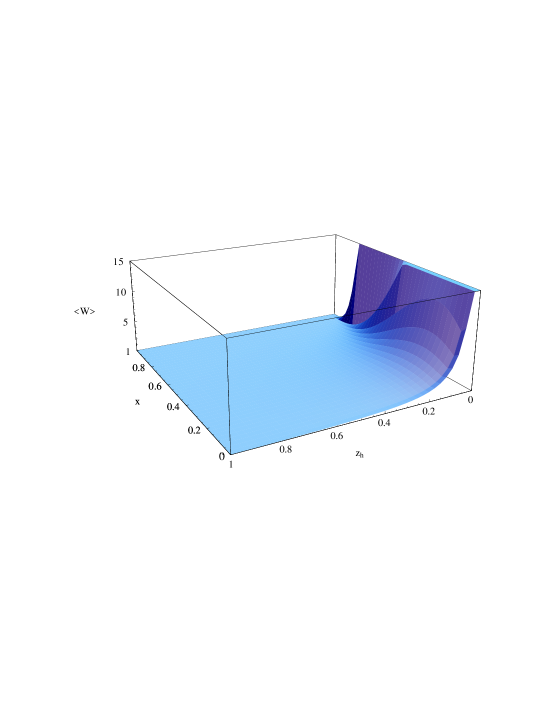
   FIG. 5.: A tri-dimensional view of the quantity $\sum_{a,\overline{a}}e_{a}^{2}\ x\,f_{1}^{a}(x)\,D_{1}^{a}(z_{h})$ as a function of $x$ and $z_{h}$. This represents the cross-section corresponding to a fully unpolarized DIS process (see Eq. 65) leading to the production of a $\pi^{+}$. Notice that only valence contributions are taken into account, for a consistent comparison with later plots. The cross-section becomes sizeable in the region in which both the variables $x$ and $z_{h}$ are relatively small.

2. If we consider $W=(Q_{T}/M)\sin(\phi^{l}_{h}-\phi^{l}_{S})$ in a scattering process with $ABC=OTO$, i.e. when an unpolarized beam hits a polarized proton target, we can single out a quantity which is directly proportional to our T-odd distribution function, or more precisely to its first moment, as given in Eq. (33) (see also Table II, last line, in Ref. [3])

   $$\left<\frac{Q_{T}}{M}\;\sin(\phi^{l}_{h}-\phi^{l}_{S})\right>_{OTO}=\frac{4\pi\alpha^{2}s}{Q^{4}}\,(1-y)\,\sum_{a,\overline{a}}e_{a}^{2}\ x\,f_{1T}^{\perp(1)a}(x)\,D_{1}^{a}(z_{h})\;.$$ (67)

   A tri-dimensional plot of the quantity $\sum_{a,\overline{a}}e_{a}^{2}\ x\,f_{1T}^{\perp(1)a}(x)\,D_{1}^{a}(z_{h})$ is shown in Fig. 6. By comparing this weighted integral to the fully unpolarized cross-section, shown in Fig. 5, we see that this time the shape of the surface as a function of $x$ and $z_{h}$ has changed, since it becomes sizeable for very small values of $z_{h}$ and intermediate values of $x$. Notice also that the overall size of the function is considerably suppressed (by roughly two orders of magnitude) by the $<k_{T}>^{2}$ factor. Therefore, it is clear that the effects due to the presence of the T-odd distribution function $f_{1T}^{\perp}(x)$ are small, but a suitably designed experiment may put limits on their existence, or might establish their mere existence. This would be a crucial test for the presence of T-odd distribution functions and provide a deeper understanding of these phenomena.

    

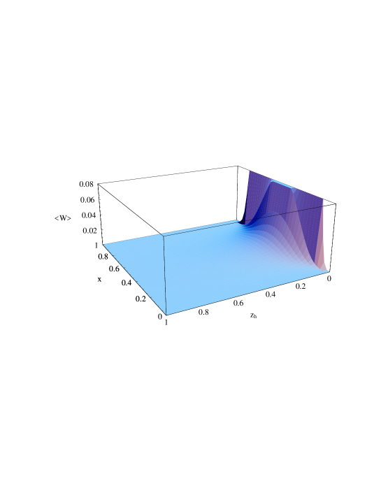
   FIG. 6.: A tri-dimensional view of the quantity $\sum_{a,\overline{a}}e_{a}^{2}\ x\,f_{1T}^{\perp(1)a}(x)\,D_{1}^{a}(z_{h})$, directly proportional to the T-odd distribution function $f_{1T}^{\perp}(x)$, see Eq. (67), for $OTO$ scattering with production of $\pi^{+}$. Only valence contributions are taken into account. Here the function becomes sizeable for small values of $z_{h}$ but intermediate values of $x$. Notice that the overall size of the surface is considerably reduced by the action of the $<k_{\scriptscriptstyle T}>^{2}$ factor.

3. Finally, if we choose the weight $W=(Q_{T}/M)\;\sin(\phi^{l}_{h}+\phi^{l}_{S})$, we obtain an object which is directly proportional to the T-odd fragmentation function $H_{1}^{\perp(1)}$ (see Table II, second line, in Ref. [3])

   $$\left<\frac{Q_{T}}{M}\;\sin(\phi^{l}_{h}+\phi^{l}_{S})\right>_{OTO}=\frac{4\pi\alpha^{2}s}{Q^{4}}\,(1-y)\,\sum_{a,\overline{a}}e_{a}^{2}\ x\,h_{1}^{a}(x)\,H_{1}^{\perp(1)a}(z_{h})\;.$$ (68)

   As it clearly appears from the plot in Fig. 7, this time the shape of the quantity $\sum_{a,\overline{a}}e_{a}^{2}x\,h_{1}^{a}(x)\,H_{1}^{\perp(1)a}(z_{h})$ as a function of $x$ and $z_{h}$ is completely different from the previous two. It reaches its maximum for relatively small values of $x$ and for large values of $z_{h}$ and its overall size is at least a factor two bigger than the previous one. This means that a measure to reveal the effects of a non zero T-odd fragmentation function could easily be made at large values of $z_{h}$, where it is relatively easier to achieve larger statistics.

    

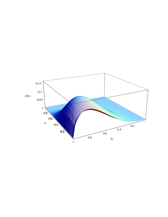
   FIG. 7.: A tri-dimensional view of $\sum_{a,\overline{a}}e_{a}^{2}x\,h_{1}^{a}(x)\,H_{1}^{\perp(1)a}(z_{h})$, directly proportional to the T-odd fragmentation function $H_{1}^{\perp}(z_{h})$, see Eq. (68), for $OTO$ scattering with production of $\pi^{+}$. Once again, only valence contributions are taken into account. As opposed to the previous case, here the function reaches its maximum for considerbly large values of $z_{h}$.

IV. EVALUATION OF THE RATIOS ${\mbox{\boldmath$H$}_{1}^{\perp}/\mbox{\boldmath$D$}_{1}}$ AND ${\mbox{\boldmath$f$}_{1T}^{\perp}/\mbox{\boldmath$f$}_{1}}$

We now focus our attention on the evaluation of the ratio $H_{1}^{\perp a}/D_{1}^{a}$, which will then be compared to the experimental results from DELPHI data on $Z\;\to\;2$ jet decay, presented by Efremov et al. in Ref. [5]. Once again we take $D_{1}(z_{h})$ from the LO fragmentation function sets by Binnewies et al. [19] and $H_{1}^{\perp}(z_{h})$ from Eq. (59). To calculate this ratio, we have to fix the flavour, $a$, of the quark; so we start by considering, for instance, $\pi^{+}$ production, in which $u$ is valence, and fix the flavour to be $u$ in our evaluation. As we can see, the integration over $z$ presents some technical problems, because the $D_{1}(z_{h})$ fragmentation function diverges at small values of $z_{h}$. Then we will perform a cut at $z_{h}(min)=0.1$ (typical cuts in HERMES and COMPASS experiments) to get a finite result. Under these assumptions we have

$$\left|\frac{\int_{0.1}^{1}\,dz_{h}\ H_{1}^{\perp\mbox{fav}}(z_{h})}{\int_{0.1}^{1}\,dz_{h}\ D_{1}^{u/\pi^{+}}(z_{h})}\right|=0.076\;.$$ (69)

This means that our evaluation of the ratio $H_{1}^{\perp a}/D_{1}^{a}$ gives a value of about $8\%$, in good agreement with the result of Ref. [5], in which the authors quote $(6.3\pm 1.7)\%$.
The calculation of Efremov et al. is averaged over the quark flavours. Since we are taking into account only valence contributions, and we are assuming isospin symmetry to hold, we have $H_{1}^{\perp\,\mbox{fav}}/D_{1}^{u/\pi^{+}}=H_{1}^{\perp\,\mbox{fav}}/D_{1}^{\bar{d}/\pi^{+}}$, then the value we give can well be compared with the averaged one. Notice that this evaluation is rather sensitive to the $z$ cut: by lowering $z_{h}(min)$ to $0.01$, for example, the ratio $H_{1}^{\perp a}/D_{1}^{a}$ would be reduced to 0.023. On the other hand, choosing a higher value of $z_{h}(min)$, say 0.2 for instance, the ratio $H_{1}^{\perp a}/D_{1}^{a}$ would increase to about 15%.

Now, a completely analogous calculation can be performed to give an estimate of the ratio $f_{1T}^{\perp}/f_{1}$. Once again we take into account only valence quarks contributions in the proton, $u$ and $d$. By adopting the same cuts as in HERMES and COMPASS experiments, $0.02\leq x\leq 0.4$, we have

$$\left|\frac{\int_{0.02}^{0.4}\,dx\,f_{1T}^{\perp\,u}(x)}{\int_{0.02}^{0.4}\,dx\,f_{1}^{u}(x)}\right|=0.083\;,$$ (70)

$$\left|\frac{\int_{0.02}^{0.4}\,dx\,f_{1T}^{\perp\,d}(x)}{\int_{0.02}^{0.4}\,dx\,f_{1}^{d}(x)}\right|=0.072\;.$$ (71)

Notice that in this case the results are not very sensitive to the $x$ cuts. In fact, we would have obtained very similar results by setting the upper limit of integration to 1 ($0.11$ and $0.08$ for $u$ and $d$ respectively). The same holds when decreasing the lower limit of integration: for $x(min)=0.01$, for example, we would have had $0.07$ for $u$ and $0.06$ for $d$.
Thus, for an average over the flavours (assuming that non-valence contributions are negligible) we find that the ratio $f_{1T}^{\perp}/f_{1}$ is about $7.7\%$, quite close to the result we found for $H_{1}^{\perp a}/D_{1}^{a}$.

We stress that none of the above estimates takes into account effects of evolution. Furthermore, just comparing integrated results neglects not only several kinematics factors, which we did show in Section III, but also forgets about experimental considerations such as azimuthal acceptances, etc.

V. CONCLUSIONS

In this paper we have presented results for some observables in lepton-proton scattering that provide information on time reversal odd distribution and fragmentation functions. Far from being precise predictions, our results give rough estimates based on experimental data from $p^{\uparrow}p$ single spin asymmetries and on some theoretical prejudice as far as unknown functions are concerned. For the two extreme possibilities, we have indicated the kinematical regions in which these rather exotic spin effects are sizeable and we have given their overall size and their relations to measurable angles ($\phi^{l}_{S}$ and $\phi^{l}_{h}$). Moreover, we find the ratio between odd and standard distribution and fragmentation functions to be of the order of a few percent. Thus, if these functions do exist, their presence could be experimentally detected.

Experimental input is now needed to deepen our knowledge on spin effects in high energy scattering processes. Once again we want to stress that only a joint effort of cooperation between theoretical modelling and experimental measurements will allow us to learn more about these soft functions, distributions and fragmentations, which in turn will teach us about the non-perturbative phenomena leading to particular correlations between quark spins and transverse momenta or phenomena occurring in the hadronization process.

REFERENCES

- [1] R. L. Jaffe and X. Ji, Nucl. Phys. B 375 (1992) 527.
- [2] R.D. Tangerman and P.J. Mulders, Phys. Rev. D51 (1995) 3357; P.J. Mulders and R.D. Tangerman, Nucl. Phys. B461 (1996) 197.
- [3] D. Boer and P.J. Mulders, Phys. Rev. D57, 5780 (1998).
- [4] A. de Ruyula, J.M. Kaplan,E de rafael, Nucl. Phys. B35 (1971) 365; K. Hagiwara, K. Hikasa, N. Kai, Phys. Rev. D27 (1983) 84; D. Atwood, G. Eilam, A. Soni, Phys. Rev. Lett. 71 (1993) 492; R.L. Jaffe and X. Ji, Phys. Rev. Lett. 71 (1993) 2547.
- [5] A.V. Efremov, O.G. Smirnova, L.G. Tkatchev, to be published on the proceedings of the XIII Int. Symp. on High Energy Spin Physics, e-print hep-ph/9812522.
- [6] R. Jacob, D. Boer and P.J. Mulders, Proceedings of the 6th International Workshop on Deep Inelastic Scattering and QCD, DIS98, Eds G.H. Coremans, R. Roosen, World Scientific 1998, p. 642.
- [7] M. Anselmino, M. Boglione and F. Murgia, Phys. Lett. B 362 (1995) 164.
- [8] M. Anselmino, A. Drago and F. Murgia, hep-ph/9703303.
- [9] J. Qiu and G. Sterman, Phys. Rev. Lett. 67 (1991) 2264, Nucl. Phys. B 378 (1992) 52; N. Hammon, O.V. Teryaev and A. Shafer, Phys. Lett. B 390 (1997) 409; D. Boer, P.J. Mulders and O.V. Teryaev, Phys. Rev. D57 (1998) 3057.
- [10] M. Anselmino, F. Murgia, Phys. Lett. B 442 (1998) 470.
- [11] M. Anselmino, M. Boglione, F. Murgia, hep-ph/9901442.
- [12] D.L. Adams et al, Phys. Lett. B261, 201 (1991) and Phys. Lett. B264, 462 (1991).
- [13] D. Sivers, Phys. Rev. D 41 (1990) 83; Phys. Rev. D 43 (1991) 261.
- [14] J. Collins, Nucl. Phys. B 396 (1993) 161.
- [15] D.E. Soper, Phys. Rev. D 15 (1977) 1141; Phys. Rev. Lett. 43 (1979) 1847; J.C. Collins and D.E. Soper, Nucl. Phys. B194 (1982) 445; R.L. Jaffe, Nucl. Phys. B 229 (1983) 205.
- [16] J.D. Jackson, G.G. Ross, R.G. Roberts, Phys. Lett. B226 (1989) 159.
- [17] P. Abreu et al., Z.Phys. C73 (1996) 11-59
- [18] A.D. Martin, W.J. Stirling, R.G. Roberts, Phys. Lett. B354, 155 (1995).
- [19] J. Binnewies, B.A. Kniehl and G. Kramer, Phys. Rev. C65, 471 (1995).