DTP/99/24

March 1999

Diagonal input for the evolution of off-diagonal partons

K.J. Golec-Biernat^a,b, A.D. Martin^a and M.G. Ryskin^a,c

^a Department of Physics, University of Durham, Durham, DH1 3LE

^b H. Niewodniczanski Institute of Nuclear Physics, ul. Radzikowskiego 152, Krakow, Poland

^c Petersburg Nuclear Physics Institute, Gatchina, St. Petersburg, 188350, Russia

We show that a knowledge of diagonal partons at a low scale is sufficient to determine the off-diagonal (or skewed) distributions at a higher scale, to a good degree of accuracy. We quantify this observation by presenting results for the evolution of off-diagonal distributions from a variety of different inputs.

1.  Introduction

Precision data are becoming available for hard scattering processes whose description requires knowledge of off-diagonal (or so-called “skewed”) parton distributions [1, 2, 3]. For example the diffractive production of vector mesons or high $E_{T}$ jets in high energy electron-proton collisions are now experimentally accessible.

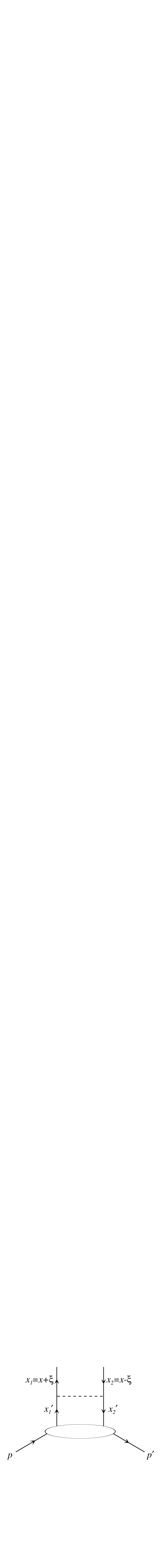
Figure 1: A schematic diagram showing the variables for the off-diagonal parton distribution $H(x,\xi)$, where $x_{1,2}=x\pm\xi$. The timelike region with $|x|<\xi$ is frequently called the ERBL domain, since in the limit $\xi\rightarrow 1$ “pure” ERBL evolution applies. Similarly $|x|>\xi$ is known as the DGLAP domain since we have “pure” DGLAP evolution for $\xi\rightarrow 0$.

Off-diagonal distributions $H(x,\xi,t,\mu^{2})$ depend on the momentum fractions $x_{1,2}=x\pm\xi$ carried by the emitted and absorbed partons at each scale $\mu^{2}$, see the lower part of Fig. 1. They also depend on the momentum transfer variable $t=(p-p^{\prime})^{2}$. However $t$ does not change as we evolve the parton distributions up in the scale $\mu^{2}$. That is $t$ lies outside the evolution and we can study the scale and $x_{i}$ dependence of $H$ for each fixed value of $t$. The evolution of the distributions $H$ with the scale is described by

$$\mu^{2}\frac{\partial H(x,\xi)}{\partial\mu^{2}}\;=\;\frac{\alpha_{S}}{2\pi}\int dx_{1}^{\prime}dx_{2}^{\prime}\>\delta(x_{1}-x_{2}-x_{1}^{\prime}+x_{2}^{\prime})\>P(x_{1}^{\prime},x_{2}^{\prime},x_{1},x_{2})\>H(x^{\prime},\xi^{\prime}),$$ (1)

see Fig. 1, where the off-diagonal splitting functions $P$ are known to leading order (LO) and the anomalous dimensions are known to next-to-leading order (NLO) accuracy. So there is a possibility to evolve $H$ numerically starting from some input distribution.

As in the diagonal case, we require the form of the starting distributions, which will be dependent on non-perturbative QCD. This poses a major problem for off-diagonal evolution since we must specify both the $x_{1}$ and $x_{2}$ behaviour of the starting distributions. We could, in principle, determine the off-diagonal input directly from data. However the possibility of determining the $x_{1}$ and $x_{2}$ behaviour, for a given $t$ value, from data is remote. Alternatively we could use some simplified model for the distributions in the non-perturbative region. Clearly it would be better to try to relate the off-diagonal distributions to their known diagonal form.

In the present paper we argue that at a low scale $\mu^{2}=Q_{0}^{2}$ one may input the diagonal forms, but smoothed in the ERBL region with $|x|<\xi$ to avoid the singularity at $x\rightarrow 0$. Then after a few steps of evolution the result will be very close to the true off-diagonal distribution. In other words the original $\xi$ dependence is washed out and forgotten during the evolution, with the final $\xi$ behaviour being generated mainly by the form of the off-diagonal splitting functions.

To some extent, the idea to use a pure diagonal input is supported by the GRV approach [7]. With more or less simple, valence-like distributions at very low input scale $Q_{0}^{2}$, the evolution generates quite reasonable diagonal parton distributions, whose $x$-dependence is essentially governed by the form of the evolution equation.

In the next section we give a better argument in favour of diagonal input at a low scale for generating reliable off-diagonal distributions by evolution. The argument is based on the polynomial properties of the operator product expansion (OPE) for the function $H(x,\xi)$.

In Section 3 we demonstrate numerically that starting at $Q_{0}^{2}=0.26$ GeV² with different inputs, which have the same diagonal limit for $\xi\rightarrow 0$, we already obtain practically the same distribution $H(x,\xi)$ in the region $Q^{2}\sim 2-10$ GeV². Thus one can reasonably specify the off-diagonal distributions directly in terms of the (conventional) diagonal partons which are known from experiment.

2.  Constraints based on the polynomial condition

First we recall the known properties of the function $H(x,\xi)$. Just from the Lorentz invariance and the tensor structure of the operators in the OPE, it follows that the $x$-moments

$$H_{n}(\xi)\;=\;\int_{-1}^{1}\>x^{n}\>H(x,\xi)\>dx\;=\;\sum_{k}^{\left[\frac{n+1}{2}\right]}\>C_{kn}\xi^{2k}$$ (2)

are even polynomials in powers of $\xi$ of order $N\leq n+1$ (i.e. $2k\leq n+1$) [4]. The odd powers of $\xi$ are absent due to the left-right $(\xi\rightarrow-\xi)$ symmetry of Fig. 1. Expanding now the off-diagonal distribution in the powers of $\xi^{2}$

$$H(x,\xi)\;=\;\sum_{k=0}^{\infty}\>\xi^{2k}\>h_{2k}(x),$$ (3)

we see that the lower moments of the coefficient functions $h_{2k}(x)$ with $n+1<2k$ are required to be zero

$$\int_{-1}^{1}\>x^{n}\>h_{2k}(x)dx\;=\;0.$$ (4)

Therefore the larger the value of $k$ the more the functions $h_{2k}(x)$ must change sign and oscillate in the interval [$-1,1$] in order to satisfy the moment conditions. These oscillations will be washed out and cancel each other during the evolution. Thus the original (input) $\xi$ behaviour will die out as $Q^{2}$ increases and only the $\xi$ dependence generated by evolution will survive.

Another way to arrive at the same conclusion is to consider the properties of the anomalous dimensions $\gamma_{n}$. Here it is better to consider the conformal moments $O_{n}$ [8]

$$O_{n}^{i}\;=\;\int\>R_{n}^{i}(x_{1},x_{2})\>H_{i}(x,\xi)\>dx,$$ (5)

with $i=q,g$, defined on the polynomial bases

$$R_{n}^{q}(x_{1},x_{2}) = \sum_{k=0}^{n}\left(\begin{array}[]{c}n\\ k\end{array}\right)\>\left(\begin{array}[]{c}n+2\\ k+1\end{array}\right)\>x_{1}^{k}\>x_{2}^{n-k}$$ (10)

$$R_{n}^{g}(x_{1},x_{2}) = \sum_{k=0}^{n}\left(\begin{array}[]{c}n\\ k\end{array}\right)\>\left(\begin{array}[]{c}n+4\\ k+2\end{array}\right)\>x_{1}^{k}\>x_{2}^{n-k}$$ (15)

with $x_{1,2}=x\pm\xi$. The conformal moments have the advantage that they do not mix during LO evolution, and are simply renormalized multiplicatively

$$O_{n}(Q^{2})\;=\;O_{n}(Q_{0}^{2})\>\left(\frac{Q^{2}}{Q_{0}^{2}}\right)^{\gamma_{n}}.$$ (16)

They satisfy the same polynomial properties as the $x$ moments of (2). So only the anomalous dimensions $\gamma_{n}$ with $n+1>2k$ may participate in the evolution of the coefficient function $h_{2k}(x)$. On the other hand the values of $\gamma_{n}$ decrease with increasing $n$. In fact $\gamma_{n}$ become negative for $n>1$. Therefore the contributions to $H(x,\xi)$ coming from the higher terms $h_{2k}(x)$ in (3) die out.

To quantify our observation we perform LO evolution of the off-diagonal distributions from a wide variety of different diagonal input distributions. We present a representative selection of our results below. To be specific we evolve from different model $(M)$ inputs based on a set of diagonal distribution at a low scale $Q_{0}$, and show, as the scale $\mu^{2}=Q^{2}$ increases, the speed with which the models tend to common off-diagonal distributions

$$\hat{H}^{M}(x,\xi,Q^{2})\;\rightarrow\;H(x,\xi,Q^{2}).$$ (17)

One possibility is simply to use the diagonal partons themselves as input

$$\hat{H}^{M}(x,\xi,Q_{0}^{2})\;=\;h_{0}(x)\;=\;f(x),$$ (18)

where $f_{q}(x)=q(x)$ and $f_{g}(x)=xg(x)$. We comment on this below.

Of course we can add to the above input distributions, functions with support entirely in the time-like ERBL region $|x|<\xi$. Evolution never pushes such functions out of the ERBL domain. On the other hand as $\xi\rightarrow 0$ such contributions become invisible and cannot be generated from diagonal parton distributions. However here we discuss functions which are analytic in the whole interval $-1\leq x\leq 1$. So far the most realistic models for the nucleon (such as [12]) are indeed analytic in the whole interval, and do not contain any $\theta(\xi-|x|)$ contributions.

For illustration we show results based on two different sets of diagonal partons. In all cases we start the off-diagonal evolution from $Q_{0}^{2}=0.26$ GeV² and show results at $Q^{2}=4$ and 100 GeV². For set 1 we take the GRV(98) partons [7] and for set 2 the toy model

$$xg\;=\;3(1-x)^{3},\quad xq\;=\;9x(1-x)^{2},\quad x\bar{q}\;=\;0,$$ (19)

which satisfies the momentum and $n_{f}=3$ flavour sum rules. Figs. 2 and 3 show the off-diagonal distributions obtained from GRV-based inputs at $\xi=0.3$ and $\xi=0.03$ respectively, whereas Figs. 4 and 5 show the corresponding distributions based on the toy model partons. In each plot the dotted curve corresponds to evolution from (unmodified) diagonal partons, as in (18). We see such an approach gives unphysical input forms in the ERBL region $|x|<\xi$, particularly for the GRV quark distribution which is singular as $x\rightarrow 0$, that is $f_{q}(x)=q(x)\sim x^{-a}$ with $a>0$. It is more realistic to smooth the input in the ERBL region. We show results for two types of smoothing, both of which retain the constraints of the polynomial condition. First the continuous curves on Figs. 2–5 are obtained by modifying the diagonal input by requiring the conformal moments (5) of $H(x,\xi,Q_{0}^{2})$ to be independent of $\xi$. Second we modify the diagonal input by using different forms of $h(y)$ in the double distribution of ref. [9]. The dashed curves are the result of one interesting choice of $h(y)$. Before we discuss the results shown in Figs. 2–5 we explain, in turn, the two smoothing procedures.

In the first case we seek an input which has the diagonal limit $H(x,\xi=0;Q_{0}^{2})=f(x,Q_{0}^{2})$, but whose conformal moments do not depend on $\xi$, that is $O_{n}(\xi)=O_{n}(0)$. This input may be calculated by the Shuvaev transform [10, 11]

$$H(x,\xi)\;=\;\int_{-1}^{1}\>dx^{\prime}\left[\frac{2}{\pi}\>{\rm Im}\>\int_{0}^{1}\>ds\>\frac{(x+\xi(1-2s))^{p}}{y(s)\sqrt{1-y(s)x^{\prime}}}\right]\>\frac{d}{dx^{\prime}}\>\left(\frac{f(x^{\prime})}{x^{\prime p}|x^{\prime}|}\right)$$ (20)

with $p=1$ for gluons and $p=0$ for quarks, where

$$y(s)\;=\;\frac{4s(1-s)}{x+\xi(1-2s)}.$$

For small values of $\xi$ and $x$ this prescription will in fact generate reliable off-diagonal distributions from known diagonal partons at any scale [11]. For large $\xi$ it should produce a more physical input than the unmodified diagonal form (18), and will much more quickly evolve into the true off-diagonal distributions. The results are shown by the continuous curves in Figs. 2–5; the smoothing of the distributions in the ERBL-region is manifest.

An alternative way to smooth out the input distributions is to use the double distributions of ref. [9]

$$H(x,\xi)\;=\;\int_{a}^{b}\>F(x-\xi y,y)\>dy$$ (21)

with

$$F(x,y)\;=\;f(x)\>h(y)\>\bigg{/}\>2\int_{0}^{1-x}\>h(y^{\prime})\>dy^{\prime}\;,$$ (22)

where $h(y)$ is an even function of $y$ and $f(x)$ is a diagonal distribution. Thus in the limit $\xi=0$ we have $H(x,\xi=0)=f(x)$. The integration limits in (21) are

$$(a,b)\;=\;\left\{\begin{array}[]{ll}\left(-\frac{1-x}{1+\xi},\frac{1-x}{1-\xi}\right)&\mbox{~{}~{}~{}~{}~{}for~{}~{}~{}~{}~{}$x>\xi$}\\ \\ \left(-\frac{1-x}{1+\xi},\frac{1+x}{1+\xi}\right)&\mbox{~{}~{}~{}~{}~{}for~{}~{}~{} $-\xi<x<\xi$ }\\ \\ \left(-\frac{1+x}{1-\xi},\frac{1+x}{1+\xi}\right)&\mbox{~{}~{}~{}~{}~{}for~{}~{}~{}~{}~{}$x<-\xi$}\;.\\ \end{array}\right.$$ (28)

This construction satisfies the polynomial condition. Indeed, if we write relation (21) in the equivalent form

$$H(x,\xi)\;=\;\int_{R}d\tilde{x}\,dy\;F(\tilde{x},y)\;\delta(x-(\tilde{x}+\xi y))\;$$ (29)

where the integration region $R$ is given by the square in the $(\tilde{x},y)$ plane defined by the vertices: $(0,\pm 1)$ and $(\pm 1,0)$, then condition (2) is explicitly satisfied.

We are free to choose the form of $h(y)$ and generate a whole range of input distributions. The choice

$$h(y)\;=\;(1-y^{2})^{p+1},$$ (30)

with $p=0,1$ for quark (gluons), generates an input form which turns out remarkably similar to that obtained by the Shuvaev transform (20). We tried several other forms for $h(y)$. A relevant choice is

$$h(y)\;=\;\sin(\pi y^{2})$$ (31)

for both quarks and gluons, since it generates an oscillatory input behaviour in the ERBL region which is qualitatively similar to the quark distribution calculated in ref. [12]. However after evolving to $Q^{2}=4$ GeV² we see that the oscillations are much weaker, and that by $Q^{2}=100$ GeV² they have already disappeared.

The similarity of the input based on (20) and (30) at scale $Q_{0}^{2}=0.26$ GeV² is fortuitous. The Shuvaev transform (20) has the advantage that it is based on conformal moments which renormalize multiplicatively, (16), with the same anomalous dimensions $\gamma_{n}$ as in the diagonal case. So the transform is stable to a change of scale, whereas this is not the case for (30). Therefore prescriptions based on (20) and (30) will give different off-diagonal distributions if applied at a higher scale.

From the representative results shown in Figs. 2–5, and from those obtained by other trial inputs based on diagonal distributions, we can draw the following conclusions.

• If we are given a set of diagonal partons $f(x,Q_{0}^{2})$ then we can predict the off-diagonal distributions $H(x,\xi,Q^{2})$ at a higher scale with a high degree of certainty. Any differences, between the prescriptions used, rapidly disappear with increasing $Q^{2}$.

• The prescriptions are most precise at small values of $\xi$, as expected from ref. [11].

• There is freedom in the form of the input distributions in the ERBL region, $|x|<\xi$, but even here the various choices evolve to a common limit reasonably rapidly with increasing $Q^{2}$, as shown, for example, by comparing the continuous and dashed curves in Figs. 2–5. (The dotted curves, corresponding to unmodified input partons, are shown simply for comparison.)

• For gluons in the whole domain, and for quarks in the DGLAP region $|x|>\xi$, the distributions evolve particularly quickly to a common limit.

These conclusions are encouraging for phenomenology. For instance they will enable data for processes described by off-diagonal distributions to provide additional independent constraints in the global (diagonal) parton analyses. For example, one type of process for which data are becoming available is high energy diffractive vector meson electroproduction. The description is dependent on the off-diagonal gluon distribution at small $x,\xi$, which is especially well known in terms of the diagonal gluon distribution, see Figs. 3 and 5.

Acknowledgements

This work was supported in part by the Royal Society, INTAS (95-311), the Russian Fund for Fundamental Research (98 02 17629), the Polish State Committee for Scientific Research grant No. 2 P03B 089 13 and by the EU Fourth Framework Programme TMR, Network ‘QCD and the Deep Structure of Elementary Particles’ contract FMRX-CT98-0194 (DG12-MIKT) and (DG12-MIHT).

Figure 2: The evolution to $Q^{2}=4$ and 100 GeV² of the quark non-singlet $H^{ns}$, the quark singlet $H^{s}$ and the gluon distribution $H_{g}(=xH_{g}^{\rm Ji})$ starting from diagonal GRV-based input at $Q_{0}^{2}=0.26$ GeV² for $\xi=0.3$. The dotted curves correspond to evolution from unmodified input partons as in (18), the continuous curves to using the “Shuvaev prescription” of (20) and the dashed curves to “double distribution” input with (31).

Figure 3: As in Fig. 2 but for $\xi=0.03$.

Figure 4: As in Fig. 2 but based on the toy model diagonal partons of (19); $\xi=0.3$.

Figure 5: As in Fig. 4 but for $\xi=0.03$.

References

- [1] D. Müller, D. Robaschik, B. Geyer, F.-M. Dittes and J. Hořejši, Fortschr. Physik 42 (1994) 101.
- [2] A.V. Radyushkin, Phys. Lett. B380 (1996) 417; Phys. Lett. B385 (1996) 333.
- [3] X. Ji, Phys. Rev. Lett. 78 (1997) 610; Phys. Rev. D55 (1997) 7114.
- [4] X. Ji, J. Phys. G24 (1998) 1181.
- [5] A.V. Radyushkin, Phys. Rev. D56 (1997) 5524.
- [6] K.J. Golec-Biernat and A.D. Martin, Phys. Rev. D59 (1999) 014029.
- [7] M. Glück, E. Reya and A. Vogt, Eur. Phys. J. C5 (1998) 461.
- [8] Th. Ohrndorf, Nucl. Phys. B198 (1982) 26.
- [9] A.V. Radyushkin, Phys. Rev. D59 (1999) 014030; hep-ph/9810466.
- [10] A.G. Shuvaev, hep-ph/9902318.
- [11] A.G. Shuvaev, K.J. Golec-Biernat, A.D. Martin and M.G. Ryskin, hep-ph/9902410.
- [12] V.Yu. Petrov et al., Phys. Rev. D57 (1998) 4325.