Form Factors and Decay Rates for Heavy $\Lambda$ Semileptonic Decays from QCD Sum Rules

Abstract

QCD sum rules for the determination of form factors of $\Lambda_{b}$ and $\Lambda_{c}$ semileptonic decays are investigated. With a form for the baryonic current appropriate for the limits of the heavy quark symmetries, the different tensor structures occurring in the two- and three-point functions are separately studied, and in each case general relations are written for the form factors. Particular attention is given to the treatment of the kinematical region ascribed to the continuum. The $t$-dependence of the form factors and the decay rates are numerically evaluated and compared to experimental information.

PACS Numbers  :  12.38.Lg , 13.30.Ce , 14.65.Dw , 14.65.Fy

1. Introduction

In this paper we treat semileptonic decays of the heavy baryons $\Lambda_{c}$ and $\Lambda_{b}$. The study of the matrix elements of weak decays of heavy hadrons are an important source of information on some elements of the Cabbibo-Kobayashi-Maskawa (CKM) matrix, but the determination of these fundamental quantities of the standard model require disentanglement from the effects of strong interactions occurring inside the hadrons.

QCD sum rules [1] (for reviews see [2, 3]) provide an important approach for calculating hadronic matrix elements and form factors for systems with both light and heavy quarks. This method deals with the nonperturbative aspects of QCD analytically using a limited input of phenomenological parameters and has been applied successfully to semileptonic decays of mesons. Unfortunately QCD sum rules are not expected to do as well for baryonic as for mesonic amplitudes. This difficulty is inherent to the method, as the basis of the sum-rule approach is an expansion in local operators. As a starting point the hadron is represented by a local interpolating field constructed from quarks. It is evident that for the case of baryons where at least three operators are taken at the same point this is a more drastic reduction than for the mesonic case with two operators. We therefore expect the contribution of higher resonances to be even more important for baryons than for mesons. Technically this reflects itself in the higher dimension of the interpolating fields and thus in a faster increase of the perturbative contribution, which makes the assumptions on the continuum contributions more decisive.

In the limit where one of the quarks in the initial and final hadrons is infinitely heavy there are new flavor and spin symmetries, which have received much attention in the last years in the framework of the so-called Heavy Quark Effective Theory (HQET) [4, 5, 6, 7, 8, 9] (for a review see [10]). QCD sum rules simplify considerably in the heavy quark limit [4], but they can be applied also to evaluate 1/M corrections to the results obtained with infinite heavy quark masses. The method has had good success in the calculation of corrections to HQET (see [10] and references therein).

In the present paper, which is an extended and revised version of a previous letter [11] we evaluate the semileptonic decays of heavy $\Lambda$-baryons in the QCD sum rule approach as it was developed a few years ago for heavy meson decays [12]. This approach treats full QCD but also reproduces the symmetries of HQET. In $\Lambda_{c}$ semileptonic decay, which is among the best investigated processes of this kind, the relevant non-Cabbibo suppressed CKM matrix element $V_{cs}$ is known, so that calculations of these decays may provide very good tests of the applied method. On the other hand, there are quite serious discrepancies between experiments and HQET in the ratios of the lifetimes of beautiful baryons to beautiful mesons (see e.g. [13]), and hence it is of prime interest to investigate in full QCD all decay channels of the $\Lambda_{b}$ baryon.

We use the sum rule technique for three-point functions that was introduced [14, 15] for the study of the pion eletromagnetic form factor at intermediate Euclidean momentum transfer. We analyse our form factors in the physical region for positive values of the momentum transfer since in this case the cut in the $t$ channel starts at $t\sim m_{Q}^{2}$ ($m_{Q}$ represents the heavy quark mass), and thus the Euclidean region stretches up to that threshold.

This paper is organized as follows: in Sec. II we discuss the method and introduce the form factors to be evaluated. In Sec. III we collect and discuss the results for the two- and three-point functions sum rules in HQET and shortly discuss the results. In Sec. IV we present our results obtained from QCD sum rules for the form factors and decay rates for $\Lambda_{c}$ and $\Lambda_{b}$ decays, and finally in Sec. V we present our conclusions. Technical details about the method used are presented in Appendices A, B and C.

2. Sum Rule Calculation

We label generically the initial channel by $I$ and the final channel by $F$. The weak transition current couples initial quark $Q_{I}$ (mass $m_{I}$) to final quark $Q_{F}$ (mass $m_{F}$), and we assume that the other two non-interacting quarks are massless ($m_{u}=m_{d}=0$.). The initial and final baryon four-momenta are called $p_{I}$ and $p_{F}$, with corresponding Mandelstam variables $s=p_{I}^{2}$ and $u=p_{F}^{2}$ respectively. The current four-momentum is called $q=p_{I}-p_{F}$, and $t=q^{2}$. We also define the four-vector $r=p_{I}+p_{F}$. The initial and final baryons are called $\Lambda_{I}$ and $\Lambda_{F}$, and their masses are $M_{\Lambda_{I}}$ and $M_{\Lambda_{F}}$.

In order to study the decay $\Lambda_{I}\to\Lambda_{F}+\ell+\nu_{\ell}$ using the QCD sum rule approach we consider the three-point function of the weak transition current from a initial to a final quark $J_{\mu}=\bar{Q}_{F}\gamma_{\mu}(1-\gamma_{5})Q_{I}$ and the interpolating fields of the initial and final baryons $\eta_{\Lambda_{I}}$ and $\eta_{\Lambda_{F}}$

$$\Pi_{\mu}(p_{F},p_{I})=i^{2}\int d^{4}xd^{4}y~{}\langle 0|T\{\eta_{\Lambda_{F}}(x)J_{\mu}(0)\overline{\eta}_{\Lambda_{I}}(y)\}|0\rangle~{}e^{ip_{F}x}e^{-ip_{I}y}\;.$$ (1)

This three-point function of two spinors and a vector and axial vector can be expressed by a superposition of scalar form factors and the 24 vector valued 4$\times$4 matrices of Table 1.

The method of sum rules is based on the simultaneous evaluation of the expression of the correlator (1) in a phenomenological representation obtained by inserting physical intermediate states (the usual spin $\frac{1}{2}$ baryons and higher resonances), and in a theoretical representation obtained through the OPE expansion. This is detailed below.

A Phenomenological Side

The phenomenological expression is continued by dispersion relations into the not-so-deep Euclidean region where $p_{F}^{2}<M_{\Lambda_{F}}^{2}$ and $p_{I}^{2}<M_{\Lambda_{I}}^{2}$ and where it is believed that the theoretical representation is reliable. We introduce the couplings $f_{I}$ and $f_{F}$ of the currents with the respective spin $\frac{1}{2}$ hadronic states

$$\langle 0|\eta_{\Lambda_{F}}|\Lambda_{F}(p_{F})\rangle = f_{F}u_{F}(p_{F})~{},$$ (2)

$$\langle\Lambda_{I}(p_{I})|\overline{\eta}_{\Lambda_{I}}|0\rangle = f_{I}\overline{u}_{I}(p_{I})\;,$$ (3)

and obtain the phenomenological representation of Eq. (1)

$$\Pi_{\mu}^{(\rm phen)}(p_{F},p_{I}) = \sum_{\rm spins}{{\langle 0|\eta_{\Lambda_{F}}|\Lambda_{F}(p_{F})\rangle}\over{p_{F}^{2}-M_{\Lambda_{F}}^{2}}}\langle\Lambda_{F}(p_{F})|J_{\mu}|\Lambda_{I}(p_{I})\rangle{{\langle\Lambda_{I}(p_{I})|\overline{\eta}_{\Lambda_{I}}|0\rangle}\over{p_{I}^{2}-M_{\Lambda_{I}}^{2}}}$$ (4)

$$+$$ higher resonances (5)

$$= \sum_{\rm spins}{{f_{F}~{}u_{F}(p_{F})}\over{p_{F}^{2}-M_{\Lambda_{F}}^{2}}}\langle\Lambda_{F}(p_{F})|J_{\mu}|\Lambda_{I}(p_{I})\rangle{{f_{I}~{}\overline{u}_{I}(p_{I})}\over{p_{I}^{2}-M_{\Lambda_{I}}^{2}}}$$ (6)

$$+ \mbox{higher resonances}\;.$$ (7)

The general transition element $\langle\Lambda_{F}(p_{F})|J_{\mu}|\Lambda_{I}(p_{I})\rangle$ with a weak current between two spin $\frac{1}{2}$ states can be written in terms of the moments $q=p_{I}-p_{F}$ and $r=p_{I}+p_{F}$, the spinors $\overline{u}_{F}(p_{F})$ and $u_{I}(p_{I})$ and the 24 structures made with $\gamma$ matrices (12 vector $v_{\mu}^{i}$ and 12 axial vector $a_{\mu}^{i}$ quantities) listed in Table I in the form

$$\langle\Lambda_{F}(p_{F})|J_{\mu}|\Lambda_{I}(p_{I})\rangle=\overline{u}_{F}(p_{F})\sum_{1}^{12}~{}\bigg{[}f_{i}^{V}~{}v_{\mu}^{i}~{}+~{}f_{i}^{A}~{}a_{\mu}^{i}\bigg{]}u_{I}(p_{I})~{}.$$ (8)

Table I

Vector and axial vector structures constructed with four-vectors $q$, $r$ and

combinations of $\gamma$ matrices. Notation is from Bjorken-Drell, with $\sigma_{\mu\nu}=\frac{i}{2}(\gamma_{\mu}\gamma_{\nu}-\gamma_{\nu}\gamma_{\mu})$.

i	$v^{i}_{\mu}$	$a^{i}_{\mu}$
1	$q_{\mu}\,1$	$q_{\mu}\,\gamma_{5}$
2	$r_{\mu}\,1$	$r_{\mu}\,\gamma_{5}$
3	$\gamma_{\mu}$	$\gamma_{\mu}\gamma_{5}$
4	$q_{\mu}\,\not\!q$	$q_{\mu}\,\not\!q\gamma_{5}$
5	$r_{\mu}\,\not\!q$	$r_{\mu}\,\not\!q\gamma_{5}$
6	$q_{\mu}\,\not\!r$	$q_{\mu}\,\not\!r\gamma_{5}$
7	$r_{\mu}\,\not\!r$	$r_{\mu}\,\not\!r\gamma_{5}$
8	$i\sigma_{\alpha\mu}q^{\alpha}$	$i\sigma_{\alpha\mu}q^{\alpha}\gamma_{5}$
9	$i\sigma_{\alpha\mu}r^{\alpha}$	$i\sigma_{\alpha\mu}r^{\alpha}\gamma_{5}$
10	$i\sigma_{\alpha\beta}q^{\alpha}r^{\beta}q_{\mu}$	$i\sigma_{\alpha\beta}q^{\alpha}r^{\beta}\gamma_{5}q_{\mu}$
11	$i\sigma_{\alpha\beta}q^{\alpha}r^{\beta}r_{\mu}$	$~{}i\sigma_{\alpha\beta}q^{\alpha}r^{\beta}\gamma_{5}r_{\mu}$
12	$~{}\epsilon_{\rho\beta\alpha\mu}q^{\rho}r^{\beta}\gamma^{\alpha}\gamma_{5}~{}$	$\epsilon_{\rho\beta\alpha\mu}q^{\rho}r^{\beta}\gamma^{\alpha}$

Since on-mass-shell $\Lambda_{I}$ and $\Lambda_{F}$ baryons obey Dirac equations

we may use the projector properties of the sums over the (on-mass-shell) spinors

$$\sum_{\rm spins}u_{I}(p_{I})\overline{u}_{I}(p_{I})=\gamma\cdot p_{I}+M_{\Lambda_{I}}~{},~{}\sum_{\rm spins}u_{F}(p_{F})\overline{u}_{F}(p_{F})=\gamma\cdot p_{F}+M_{\Lambda_{F}}~{},$$ (9)

and the sum over 24 invariants in Eq. (8) can be reduced to only 6 independent terms.

The experimental information is usually represented [16] by the invariant decomposition of the amplitude in the form

$$\langle\Lambda_{F}(p_{F})|J_{\mu}|\Lambda_{I}(p_{I})\rangle =$$ (11)

$$\overline{u}(p_{F})[\gamma_{\mu}(F_{1}^{V}+F_{1}^{A}\gamma_{5})+i\sigma_{\mu\nu}q^{\nu}(F_{2}^{V}+F_{2}^{A}\gamma_{5})+q_{\mu}(F_{3}^{V}+F_{3}^{A}\gamma_{5})]u(p_{I})\;,$$

where the form factors $F^{V,A}_{i}~{}~{}(i=1,2,3)$ are functions of $t=q^{2}$ .

We then obtain for the phenomenological representation of the correlator

$$\Pi_{\mu}^{(\rm phen)}(p_{F},p_{I}) = {(f_{F}\hbox to0.0pt{/\hss}{p_{F}}+f^{\prime}_{F})\over p_{F}^{2}-M_{\Lambda_{F}}^{2}}~{}\bigg{[}\gamma_{\mu}(F_{1}^{V}+F_{1}^{A}\gamma_{5})+i\sigma_{\mu\nu}q^{\nu}(F_{2}^{V}+F_{2}^{A}\gamma_{5})$$ (12)

$$+ q_{\mu}(F_{3}^{V}+F_{3}^{A}\gamma_{5})\bigg{]}~{}{(f_{I}\hbox to0.0pt{/\hss}{p_{I}}+f^{\prime}_{I})\over p_{I}^{2}-M_{\Lambda_{I}}^{2}}+\mbox{higher resonances}\;,$$ (13)

where we have defined

$$f^{\prime}_{F}=f_{F}M_{\Lambda_{F}}~{}~{},~{}~{}f^{\prime}_{I}=f_{I}M_{\Lambda_{I}}~{}.$$ (14)

The reason for the separate notations for $f$ and $f^{\prime}$ is that they belong to terms with different spin content (with and without $\gamma$ matrix) and this will help in the classification of types of traces to be evaluated. Another reason is that we shall determine $f$ and $f^{\prime}$ from the mass sum rules for $\Lambda_{I}$ and $\Lambda_{F}$, and there is no guarantee that we have exactly $f^{\prime}_{I}=f_{I}M_{\Lambda_{I}}$, $f^{\prime}_{F}=f_{F}M_{\Lambda_{F}}$ .

Referring to the spinor forms that appear in Eq. (13), we may pick up terms with or without $\gamma$ matrices in the numerators of the two fractions, and thus form four different kinds of products that we identify as

$$F^{V,A}_{i}(q^{2})f_{I}f_{F}~{},~{}F^{V,A}_{i}(q^{2})f_{I}f^{\prime}_{F}~{},~{}F^{V,A}_{i}(q^{2})f^{\prime}_{I}f_{F}~{},~{}F^{V,A}_{i}(q^{2})f^{\prime}_{I}f^{\prime}_{F}~{},~{}~{}({\rm with}~{}i=1,2,3)~{}.$$ (15)

We project out a sum rule for each one of these 24 products by performing appropriate traces using Eq. (13). Independent traces can be formed after multiplying Eq. (13) by the 12 vector and 12 axial-vector structures of Table I

$$x_{i}\equiv\mbox{ Tr }[v^{i}_{\mu}\Pi^{\mu,(\rm phen)}]\mbox{~{} and ~{} }u_{i}\equiv\mbox{ Tr }[a^{i}_{\mu}\Pi^{\mu,(\rm phen)}],\quad i=1,\dots 12~{},$$ (16)

so that we obtain $2\times 12$ independent relations that must be solved for the $2\times 12$ unknowns quantities mentioned in Eq. (15) (we must recall that before we must introduce $q$ and $r$ everywhere in the places of $p_{I}$, $p_{F}$). The results are given in Appendix A.

The constants $f_{I}$, $f^{\prime}_{I}$, $f_{F}$, and $f^{\prime}_{F}$ have to be calculated from two-point function sum rules, as usual.

B Theoretical Side

The theoretical counterpart is evaluated by performing the Wilson’s operator product expansion (OPE) of the operator in Eq. (1) and then taking the expectation value with respect to the physical vacuum. The term from the unit operator gives the usual perturbative contribution, while the vacuum expectation values of the other operators in the expansion give the nonperturbative corrections proportional to the condensates of the respective operators. Thus

$$\Pi^{(\rm theor)}_{\mu}=\Pi^{(\rm pert)}_{\mu}+\sum_{i}\Pi^{({\rm nonpert}(i))}_{\mu}~{},$$ (17)

where the index $i$ refers to the types and dimensions of the condensates.

As usual in the sum rule method, we wish to evaluate the form factors that build the $\langle\Lambda_{F}|J_{\mu}|\Lambda_{I}\rangle$ amplitude by matching the phenomenological representation Eq. (13) of the three point function with its theoretical counterpart from Eq. (17). The higher resonances are approximated by the perturbative contribution invoking quark hadron duality [1].

As it is well known from two-point sum rules for baryons [17, 18, 19], there is a continuum of choices for the interpolating currents. Of course the results should in principle be independent of the choice of the current (except for pathological cases which couple very weakly to the ground state), but the justification of the approximations depends on the choice made. From the point of view of heavy quark symmetries, the spin of the heavy $\Lambda$ is carried by the heavy quark, with the light quarks being in a spin and isospin singlet state, namely

$$\eta_{\Lambda_{Q}}=\epsilon_{ABC}(\bar{u}^{A}\gamma^{5}d^{B})Q^{C}~{},$$ (18)

where $u^{A}$ and $d^{B}$ stand for the Dirac fields of light quarks of colors $A$ and $B$, and $Q^{C}$ represents a heavy quark ($b$ or $c$) of color $C$. This current couples strongly to the $\Lambda$ states in the heavy quark limit, and with this choice the quark condensate and the mixed quark-gluon condensate do not contribute to Eq. (17). The gluon condensate does contribute, but experience with baryonic two-point functions and mesonic three point functions teaches us that it is of little influence. We are thus left with only the perturbative and the four quark condensate contributions.

Once we have calculated explicitly the terms contributing to $\Pi_{\mu}^{(\rm theor)}$ we can form the traces

$$x_{i}\equiv\mbox{ Tr }[v^{i}_{\mu}\Pi^{\mu,{(\rm theor)}}]\mbox{~{} and ~{} }u_{i}\equiv\mbox{ Tr }[a^{i}_{\mu}\Pi^{\mu,{(\rm theor)}}],\quad i=1,\dots 12~{},$$ (19)

and thus project out the form factors given in Appendix A.

C Sum Rule

To the 24 invariants in Eq. (8) correspond in the off-mass-shell case 24 invariant functions $F_{i}^{V,A}(s,u,t)f_{I}^{(^{\prime})}f_{F}^{(^{\prime})}$ (where by $f_{I}^{(^{\prime})}$ we mean either $f_{I}$ or $f^{\prime}_{I}$, and similarly for $f_{F}^{(^{\prime})}$ ) given in Appendix A. They obey double dispersion relations of the form

$$F_{i}^{V,A}(s,u,t)f_{I}^{(^{\prime})}f_{F}^{(^{\prime})}={1\over\pi^{2}}\int_{m_{I}^{2}}^{\infty}ds^{\prime}\int_{m_{F}^{2}}^{\infty}du^{\prime}{\rho_{i}^{V,A}(s^{\prime},u^{\prime},t)\over(s^{\prime}-s)(u^{\prime}-u)}+\cdot\cdot\cdot\;,$$ (20)

where $-4\rho_{i}^{V,A}(s,u,t)$ equals the double discontinuity of the amplitude $F_{i}^{V,A}(s,u,t)f_{I}^{(^{\prime})}f_{F}^{(^{\prime})}$ on the cuts $m_{I}^{2}\leq s<\infty$, $m_{F}^{2}\leq u<\infty$, which is given by the double discontinuity of the right hand side of the expressions in Appendix A. In Eq. (20) $m_{I}$ and $m_{F}$ are respectively the initial and final heavy quark masses and the dots represent subtraction polynomials in $s$ and $u$, which will vanish under the double Borel transform [14], in a straightforward generalization of that used before [1]. Applying the double Borel transform to Eq.(20) and subtracting the continuum contribution we obtain

$$F_{i}^{V,A}(t)f_{I}^{(^{\prime})}f_{F}^{(^{\prime})}e^{-M_{\Lambda_{I}}^{2}/M_{I}^{2}}e^{-M_{\Lambda_{F}}^{2}/M_{F}^{2}} = {1\over\pi^{2}}\int_{m_{I}^{2}}^{\infty}ds^{\prime}\int_{m_{F}^{2}}^{\infty}du^{\prime}R_{cont}(s^{\prime},u^{\prime},s_{0},u_{0})$$ (22)

$$\times\rho_{i}^{V,A}(s^{\prime},u^{\prime},t)e^{-s^{\prime}/M_{I}^{2}}e^{-u^{\prime}/M_{F}^{2}}\;,$$

where $M_{I}^{2}$ and $M_{F}^{2}$ are the Borel parameters and $R_{cont}(s^{\prime},u^{\prime},s_{0},u_{0})$ defines the continuum model with $s_{0}$ and $u_{0}$ being, respectively, the continuum thresholds for the $\Lambda_{I}$ and $\Lambda_{F}$ baryons, determined from the mass sum rules.

We will consider two different region of integration for the continuum contribution. A rectangular region specified by a rectangular cutoff:

$$R_{cont}(s^{\prime},u^{\prime},s_{0},u_{0})=\Theta(s_{0}-s^{\prime})\Theta(u_{0}-u^{\prime})\;,$$ (23)

and a triangular region determined by:

$$R_{cont}(s^{\prime},u^{\prime},s_{0},u_{0})=\Theta\left(u_{0}-\frac{m_{F}}{m_{I}}(s^{\prime}-s_{0})-u^{\prime}\right)\;.$$ (24)

In the OPE side of the sum rules we can evaluate the double discontinuity of the traces $x_{i}$ using Cutkosky’s rules. The perturbative contribution to the double discontinuity of $x_{i}$ in Eq.(19) is given by

$${\cal DD}[x_{i}]_{\rm(pert)} = -{6\over(2\pi)^{3}}{1\over 8\sqrt{\lambda(s,u,t)}}\int_{0}^{(\sqrt{s}-m_{I})^{2}}dm^{2}\;m^{2}\int dK_{0}d{|\vec{K}|}^{2}d\cos\theta_{K}d\phi_{K}$$ (26)

$$\times\delta(K_{0}-\overline{K}_{0})\delta(|\vec{K}|^{2}-\overline{|\vec{K}|^{2}})\delta(\cos\theta_{K}-\overline{\cos\theta_{K}})\Theta(1-\overline{\cos\theta_{K}}^{2})N_{i}\;,$$

where

$$\overline{K}_{0}=(s+m^{2}-m_{I}^{2})/2\sqrt{s}~{}~{},~{}~{}\overline{|\vec{K}|^{2}}=\lambda(s,m^{2},m_{I}^{2})/4s$$

and

$$\overline{\cos\theta_{K}}={2p_{s_{0}}\overline{K}_{0}-u-m^{2}+m_{F}^{2}\over 2|\vec{p_{s}}||\vec{K}|}\;,$$ (27)

where

$$p_{s_{0}}=(s+u-t)/2\sqrt{s}~{},~{}|\vec{p_{s}}|^{2}=\lambda(s,u,t)/4s$$

and

$$\lambda(x,y,z)=x^{2}+y^{2}+z^{2}-2xy-2xz-2yz~{}.$$

In Eq.(26) $N_{i}$ represents the traces of the Lorentz structure of the three-point function multiplied by each of the 12 independent vector structures $v_{i}^{\mu}$

$$N_{i}=\mbox{ Tr }[(\hbox to0.0pt{/\hss}{p_{s}}-\hbox to0.0pt{/\hss}{K}+m_{F})\gamma_{\mu}(1-\gamma_{5})(\hbox to0.0pt{/\hss}{p_{c}}-\hbox to0.0pt{/\hss}{K}+m_{I})v_{i}^{\mu}]\;.$$ (28)

There are, of course, equivalent expressions for the double discontinuity of $u_{i}$ (see Eq.(19)) where the Lorentz structure is multiplied by the axial vector quantities $a_{i}^{\mu}$.

In order to estimate the four-quark condensate we use the factorization

$$\langle\bar{d}^{A}_{\alpha}\bar{u}^{B}_{\beta}u^{B^{\prime}}_{\beta^{\prime}}d^{A^{\prime}}_{\alpha^{\prime}}\rangle={\kappa\over 12^{2}}~{}\delta_{\beta\beta^{\prime}}\delta_{\alpha\alpha^{\prime}}\delta^{AA^{\prime}}\delta^{BB^{\prime\prime}}\langle\bar{u}u\rangle\langle\bar{d}d\rangle~{},$$ (29)

where the parameter $\kappa$, which may have some value from $1$ to $3$, is introduced to account for deviations from the factorization hypothesis [2].

For the particular choice of current shown in Eq. (18) and using only the sum rules based on $f_{I}$ and $f_{F}$ structures (for which the imaginary parts are positive definite) we obtain the general results

$$F^{A}_{1}(t)=-\,F^{V}_{1}(t)~{};\;F^{V}_{2}(t)=F^{V}_{3}(t)=F^{A}_{2}(t)=F^{A}_{3}(t)=0\;,$$ (30)

with the $t$-dependence given by

$$F_{1}^{V}(t) = {\frac{e^{M_{\Lambda_{I}}^{2}/M_{I}^{2}}e^{M_{\Lambda_{F}}^{2}/M_{F}^{2}}}{20\pi^{4}f_{I}f_{F}}}\bigg{[}{15\over 16}\int_{m_{I}^{2}}^{\infty}ds^{\prime}\int_{m_{F}^{2}}^{\infty}du^{\prime}{\frac{P(s^{\prime},u^{\prime},t)}{[\lambda(s^{\prime},u^{\prime},t)]^{5/2}}}e^{-s^{\prime}/M_{I}^{2}}e^{-u^{\prime}/M_{F}^{2}}$$ (32)

$$\Theta(u^{\prime}-u_{\rm min})\Theta(u_{\rm max}-u^{\prime})\;R_{cont}(s^{\prime},u^{\prime},s_{0},u_{0})+{10\over 3}\pi^{4}\kappa\langle\overline{q}q\rangle^{2}e^{-m_{I}^{2}/M_{I}^{2}}e^{-m_{F}^{2}/M_{F}^{2}}\bigg{]}~{},$$

where

$$P(s,u,t)={1\over 2}\{m_{I}^{4}u+s[m_{F}^{4}+m_{F}^{2}(s-t-u)+tu]-m_{I}^{2}[(s+t-u)u+m_{F}^{2}(s-t+u)]\}^{2}~{},$$ (33)

and the quantities

$$u_{{\begin{array}[]{l}{\rm min}\\ {\rm max}\end{array}}}={1\over 2m_{F}^{2}}\left\{m_{F}^{2}(s+m_{I}^{2})+(s-m_{I}^{2})\left[m_{I}^{2}-t\mp\sqrt{\lambda(m_{I}^{2},m_{F}^{2},t)}\right]\right\}\;,$$ (34)

define the physical region.

As mentioned before, $f_{I}$ and $f_{F}$ are determined from the two point sum rules and are given by [19]

$$f_{I(F)}^{2} = {e^{M_{\Lambda_{I(F)}}^{2}/M_{MI(MF)}^{2}}\over 20\pi^{4}}\left[{5\over 128}m_{I(F)}^{4}\int_{m_{I(F)}^{2}}^{s_{0}(u_{0})}ds~{}h(s)~{}e^{-s/M_{MI(MF)}^{2}}\right.$$ (35)

$$+ {5\over 768}\langle g_{s}^{2}G^{2}\rangle\int_{m_{I(F)}^{2}}^{s_{0}(u_{0})}ds~{}(1-x)(1+5x^{2})~{}e^{-s/M_{MI(MF)}^{2}}+\left.{10\over 3}\pi^{4}\kappa\langle\overline{q}q\rangle^{2}e^{-m_{I(F)}^{2}/M_{MI(MF)}^{2}}\right]\;,$$ (36)

with

$$h(s)=(1-x^{2})\left(1-{8\over x}+{1\over x^{2}}\right)-12\ln{x}\;,$$ (37)

where

$$x=m_{I(F)}^{2}/s~{},$$

while $M_{MI(MF)}$ represent the Borel masses in the two-point functions of $\Lambda_{I}$ and $\Lambda_{F}$ respectively. In Eq. (36) we have included the gluon condensate, $\langle g_{s}^{2}G^{2}\rangle$, contribution for completeness, but its contribution is negligible and does not influence meaningfully the actual calculation.

Comparing Eqs. (32) and (36) we can see that the exponentials multiplying Eq. (32) disappear if we choose

$$2M_{MI(MF)}^{2}=M_{I(F)}^{2}~{}.$$ (38)

Indeed, this way of relating the Borel parameters in the two- and three-point functions is a crucial ingredient for the incorporation of the HQET symmetries, and leads to a considerable reduction of the sensitivity to input parameters, such as continuum thresholds $s_{0}$ and $u_{0}$, and to radiative corrections [20].

3. Leading HQ limit

In the HQET limit for infinite quark masses, the expressions for the sum rules simplify considerably, as was first noted by Shuryak[4]. All form factors can be described in terms of a simple function, the Isgur-Wise (IW) function, $\xi$, normalized to 1 at maximum momentum transfer. We use the familiar $y$-variable, related to the square of momentum transfer by

$$t=m_{I}^{2}+m_{F}^{2}-2m_{I}\,m_{F}~{}y~{}.$$ (39)

For convenience we give the relation between the Dirac-type form factors used here and the velocity form factors appropriate for HQET. The latter are defined through

$$\langle\Lambda_{F}(p_{F})|J_{\mu}|\Lambda_{I}(p_{I})\rangle =$$ (41)

$$\bar{u}(p_{F})\left(\gamma_{\mu}G^{V}_{1}+v_{\mu}^{I}G^{V}_{2}+v_{\mu}^{F}G^{V}_{3}+\gamma_{5}(\gamma_{\mu}G^{A}_{1}+v_{\mu}^{I}G^{A}_{2}+v_{\mu}^{F}G^{A}_{3})\right)u(p_{I})~{},$$

where $v^{I}$ and $v^{F}$ are the velocities of the initial and final hadron respectively, and the form factors are functions of $y$.

Neglecting the matching conditions one has $G^{V}_{1}\,=\,G^{A}_{1}\,=\xi(y)+O\left(\frac{1}{m}\right)$, and all other form factors are $O\left(\frac{1}{m}\right)$   . The relations with the form factors defined in Eq. (11) are given by [10, 16]

$$F^{V}_{1}(t) = G^{V}_{1}+(m_{F}+m_{I})\left(\frac{1}{2m_{I}}G^{V}_{2}+\frac{1}{2m_{F}}G^{V}_{3}\right)~{},$$ (42)

$$F^{V}_{2}(t) = -\frac{1}{2m_{I}}G^{V}_{2}-\frac{1}{2m_{F}}G^{V}_{3}~{},$$ (43)

$$F^{V}_{3}(t) = -\frac{1}{2m_{I}}G^{V}_{2}+\frac{1}{2m_{F}}G^{V}_{3}~{},$$ (44)

$$F^{A}_{1}(t) = -G^{A}_{1}-(m_{F}-m_{I})\left(\frac{1}{2m_{I}}G^{A}_{2}+\frac{1}{2m_{F}}G^{A}_{3}\right)~{},$$ (45)

$$F^{A}_{2}(t) = \frac{1}{2m_{I}}G^{A}_{2}+\frac{1}{2m_{F}}G^{A}_{3}~{},$$ (46)

$$F^{A}_{3}(t) = \frac{1}{2m_{I}}G^{A}_{2}-\frac{1}{2m_{F}}G^{A}_{3}~{}.$$ (47)

The baryonic two-point functions were discussed both in full QCD and in the HQ-limit in ref. [19], three-point functions in ref. [21], and 1/m corrections have been considered in ref. [22].

In this section we collect and discuss the results for the two- and three-point sum rules. We stay on the firm grounds of Wilson’s OPE and only use local condensates. The four-quark condensate, which is the most important non-perturbative input, is normally reduced to the square of the chiral symmetry breaking two-quark condensate through the factorization hypothesis. We allow for an uncertainty in the factorization hypothesis introducing a factor $\kappa$ that takes some value between 1 and 3 (see Eq.(29)).

Usually one introduces the variables $\omega$ and $\mu$ related to the relativistic momentum square $s$ and the variable $M^{2}$ which appears after Borel improvement by

$$s=m^{2}+2m\omega~{}~{};\qquad M^{2}=2m\mu~{},$$ (48)

where $m$ represents the heavy quark mass ($m_{I}$ or $m_{F}$). Then the square of the coupling to the $\Lambda$ current ($\hbox to0.0pt{/\hss}{q}$- structure) is given by the sum rule derived from the two-point function

$$f^{2}=\exp\left[\frac{M_{\Lambda}^{2}-m^{2}}{2m\mu}\right]\frac{1}{20\pi^{4}}\left(I_{5}(\mu)+\frac{5}{32}\langle g_{s}^{2}G^{2}\rangle I_{1}(\mu)+\frac{10}{3}\pi^{4}\kappa\langle\bar{q}q\rangle^{2}\right)+O\left(\frac{1}{m}\right)\;,$$ (49)

with

$$I_{n}(\mu)=\int_{0}^{\omega_{c}}\omega^{n}e^{-\omega/\mu}d\omega~{}.$$ (50)

Here the cutoff $\omega_{c}$ is the continuum threshold, i.e, above this value the resonances are taken into account by perturbation theory. One can easily see that Eq. (49) is obtained from Eq. (36) when the limit $m_{I(F)}\rightarrow\infty$ is taken and the relations of form factors in Eq. (47) are used.

In order to ensure Luke’s theorem [23] for the three-point function one has to ensure that the two-point sum rule yields a correct difference between the baryon and quark masses. Using the reasonable values $m_{b}=4.7$ GeV and $m_{c}$=1.35 GeV we obtain 0.94 GeV for the mass difference when the cutoff and Borel parameters take respectively the values $\omega_{c}=1.4$ and $\mu=1~{}\nobreak\,\mbox{GeV}$ or $\omega_{c}=1.3$ and $\mu=2~{}\nobreak\,\mbox{GeV}$.

FIG. 1.: Quark-hadron duality in HQET. The physical region for the three-point function with heavy hadrons for a fixed value of y is the wedge between thesolid lines. According to ref.[25] duality can only be assumed after integration over the variable $\omega=\omega_{1}-\omega_{2}$, namely along the dotted lines.

In order to determine the Isgur-Wise (IW) function, the choice of the continuum model is very important. As has been argued by Neubert [24] and shown in detail in a non-relativistic model by Blok and Shifman [25] it is essential to use a triangular cutoff in order to take into account correctly the contributions of the higher resonances, since a rectangular cutoff yields non-analytic behavior of the IW function at $y=1$ and, as has been shown at least in the model consideration in ref. [25], quark hadron duality for the three-point holds only after the double spectral function is integrated along the dotted lines in Fig. 1. Performing this integration along the lines $\omega=(\omega_{1}+\omega_{2})/2={\rm const}$, we are left with the sum rule for the three-point function, depending only on the Borel variable $\mu$ corresponding to $\omega$, and the IW function is given by

$$\xi(y) = \left(\frac{8}{(1+y)^{3}}I_{5}(\mu)+\frac{5}{32}\langle g_{s}^{2}G^{2}\rangle I_{1}(\mu)\,\frac{2}{1+y}[1+\frac{1}{3}\frac{y-1}{1+y}]+\frac{10}{3}\pi^{4}\kappa\langle\bar{q}q\rangle^{2}\right)$$ (51)

$$\times \left(I_{5}(\mu)+\frac{5}{32}\langle g_{s}^{2}G^{2}\rangle I_{1}(\mu)+\frac{10}{3}\pi^{4}\kappa\langle\bar{q}q\rangle^{2}\right)^{-1}+O\left(\frac{1}{m}\right)\;.$$ (52)

As discussed before, we have chosen the nonrelativistic Borel parameters for the three-point function to be twice the value of the two-point channel (here we have assumed the Borel parameters to be the same in the initial and final channels); this condition is essential for correct normalization. It can be shown that Eq. (32) reduces to Eq. (52) when the limit $m_{I(F)}\rightarrow\infty$ is taken.

FIG. 2.: Isgur-Wise function at $y$=1.5 as function of the Borel parameter $\mu$.

FIG. 3.: IW function (solid line) and its derivative (dashed line) as function of $y$ for $\mu=1$ GeV and $\omega_{c}$ = 1.4 GeV.

In Fig. 2 we show that the IW function at $y=1.5$ as a function of the Borel parameter $\mu$ in the range from 1 to 2 GeV presents a reasonable stability. In Fig. 3 we display the IW function $\xi(y)$ and its slope $\xi^{\prime}(y)$ in the phenomenologically interesting range for $y$ from 1 to 1.5. The influence of the choice of the parameters can be read off from Table II, where we show the values of $\xi(1.5)$ and of the slope $\xi^{\prime}(1)$.

Table II

Values of the IW function $\xi$ at $y=1.5$ and of its slope $\xi^{\prime}$

at $y=1$ for different values of the parameters.

	$\mu$	$\omega_{c}$	$\xi(1.5)$	$\xi^{\prime}(1)$
	(GeV)	(GeV)
standard set	1	1.4	0.638	-1.098
standard set	2	1.3	0.630	-1.119
standard set	1	1.6	0.592	-1.242
no gluon condensate	1	1.4	0.609	-1.199
no four-quark condensate	1	1.4	0.560	-1.333
no four-quark condensate	1	1.15	0.599	-1.202

We see that the strongest influences come from the choices of the cutoff $\omega_{c}$ and of the four-quark condensate, and also that the influence of the gluon condensate is small.

We can represent the sum rule result for the IW function accurately through a pole fit

$$\xi(y)=\frac{1}{1+1.136(y-1)}~{}.$$ (53)

It is important to remark that the slope of the IW function varies appreciably in the range $1\leq y\leq 1.5$ as can be seen in the dashed line in Fig. 3. Our result for the slope at maximum momentum transfer is about twice the value obtained in ref. [22] where a linear fit is used. The slope at maximum momentum transfer is potentially important for model insensitive determinations of $V_{cb}$ [26] from $\Lambda_{b}$ semileptonic decays.

FIG. 4.: IW function as function of the momentum transfer $t$ (see Eq. (39)) (solid line). The dashed line shows the same function with $t$ and $y$ related by the physical masses, as given in Eq. (54).

In order to compare with the results of the full QCD sum rules for the $\Lambda_{b}\to\Lambda_{c}\ell\nu_{\ell}$ decay we plot in Fig. 4 the IW function of Eq. (52) as a function of $t$ (solid line); the dashed line shows the IW function as a function of $t$ when $t$ and $y$ are related with the physical hadron (and not the quark) masses through

$$t=M_{\Lambda_{b}}^{2}+M_{\Lambda_{c}}^{2}-2M_{\Lambda_{b}}M_{\Lambda_{c}}y~{}.$$ (54)

4. Form Factors and Decay Rates in full QCD

In this section we discuss the results for the structure $f_{I}f_{F}$. The results based on the structures $f^{\prime}_{I}f_{F}$ and $f_{I}f^{\prime}_{F}$ are given respectively in Appendices B and C.

In order to determine the continuum thresholds $u_{0}$ and $s_{0}$ for the form factors and decay rates in full QCD we first analyse the mass sum rules. The expression for the two point sum rule in the $\hbox to0.0pt{/\hss}{q}$-structure was given in Eq. (36). The corresponding sum rule in the $\bf{1}$-structure is given by [19]

$$f_{I(F)}^{2}M_{\Lambda_{I(F)}} = {e^{M_{\Lambda_{I(F)}}^{2}/M_{MI(MF)}^{2}}\over 16\pi^{4}}\left[{1\over 8}m_{I(F)}^{5}\int_{m_{I(F)}^{2}}^{s_{0}(u_{0})}ds~{}g(s)e^{-s/M_{MI(MF)}^{2}}\right.$$ (55)

$$+ {m_{I(F)}\over 96}\langle g_{s}^{2}G^{2}\rangle\int_{m_{I(F)}^{2}}^{s_{0}(u_{0})}ds~{}g_{G}(s)e^{-s/M_{MI(MF)}^{2}}+\left.{8\over 3}\pi^{4}m_{I(F)}\kappa\langle\overline{q}q\rangle^{2}e^{-m_{I(F)}^{2}/M_{MI(MF)}^{2}}\right]\;,$$ (56)

with

$$g(s) = (1-x)\left(1+{10\over x}+{1\over x^{2}}\right)+6\left(1+{1\over x}\right)\ln{x}\;,$$ (57)

$$g_{G}(s) = (1-x)\left(7+{2\over x}\right)+6\ln{x}\;,$$ (58)

where $x=m_{I(F)}^{2}/s$.

FIG. 5.: $\Lambda_{b}$ mass obtained from the mass sum rules, as function of the Borel mass squared for three different values of the continuum threshod $s_{0}=(5.65\nobreak\,\mbox{GeV}+\Delta_{s})^{2}$: $\Delta_{s}=0.4\nobreak\,\mbox{GeV}$ (dotted line), $\Delta_{s}=0.5\nobreak\,\mbox{GeV}$ (solid line) and $\Delta_{s}=0.6\nobreak\,\mbox{GeV}$ (dashed line).

In Fig. 5 we show $M_{\Lambda_{b}}$ as a function of the Borel mass $M_{Mb}$, obtained by dividing Eq. (56) by Eq. (36) for different values of

$$s_{0}=(M_{\Lambda_{b}}+\Delta_{s})^{2}\;.$$ (59)

The parameter values used in all calculations are $m_{b}=4.6$ GeV, $m_{c}=1.4$ GeV, $M_{\Lambda_{c}}=2.285$ GeV, $M_{\Lambda_{b}}=5.65$ GeV and $\langle\bar{q}q\rangle=-(230\;{\rm MeV})^{3}$, and we have neglected the gluon condensate. As can be seen in this figure, there is a rather stable plateau for $M_{Mb}^{2}\geq 10~{}\nobreak\,\mbox{GeV}^{2}$, for the three values of $s_{0}$ considered. A similar result is obtained for $M_{\Lambda_{c}}$, with a stable plateau for $M_{Mc}^{2}\geq 4~{}\nobreak\,\mbox{GeV}^{2}$ as shown in Fig. 6, where we plot $M_{\Lambda_{c}}$ versus the Borel mass $M_{Mc}$, for three different values of

$$u_{0}=(M_{\Lambda_{c}}+\Delta_{u})^{2}\;.$$ (60)

FIG. 6.: $\Lambda_{c}$ mass obtained from the mass sum rules, as a function of the Borel mass squared for three different values of the continuum threshod $u_{0}=(2.285\nobreak\,\mbox{GeV}+\Delta_{u})^{2}$: $\Delta_{u}=0.6\nobreak\,\mbox{GeV}$ (dotted line), $\Delta_{u}=0.7\nobreak\,\mbox{GeV}$ (solid line) and $\Delta_{u}=0.8\nobreak\,\mbox{GeV}$ (dashed line). The less stable result in the dot-dashed line is obtained for $\kappa=2$ (see Eq.(29)) and $\Delta_{u}=0.8\nobreak\,\mbox{GeV}$.

In Figs. 5 and 6 we have considered $\kappa=1$. A larger value of $\kappa$ decreases the value of $M_{\Lambda_{b(c)}}$ and makes the curve less stable, as shown by the dashed-dotted line in Fig. 6, where we have used $\kappa=2$ and $\Delta_{u}=0.8$ GeV.

In ref. [18] it was argued that the determination of the baryon mass based on the ratio of Eqs. (56) and (36) may be misleading especially for light baryons, since states with positive and negative parity contribute to it with opposite signs (we shall call this method 1). An alternative way to determine the baryon mass is based on the sum rule Eq. (36) and its derivative with respect to $M_{M}^{-2}$ that yield

$$f_{I(F)}^{2}M_{\Lambda_{I(F)}}^{2} = {e^{M_{\Lambda_{I(F)}}^{2}/M_{MI(MF)}^{2}}\over 20\pi^{4}}\left[{5\over 128}m_{I(F)}^{4}\int_{m_{I(F)}^{2}}^{s_{0}(u_{0})}ds~{}s~{}h(s)~{}e^{-s/M_{MI(MF)}^{2}}\right.$$ (61)

$$+ \left.{10\over 3}\pi^{4}\kappa\langle\overline{q}q\rangle^{2}m_{I(F)}^{2}e^{-m_{I(F)}^{2}/M_{MI(MF)}^{2}}\right]\;,$$ (62)

with $h(s)$ given by Eq. (37). Using the square root of the ratio between Eqs. (62) and (36) to determine $M_{\Lambda_{I(F)}}$ (method 2) we have obtained curves very similar to the ones shown in Figs. 5 and 6, but with lower continuum thresholds. For instance, we cannot distinguish the solid lines in Figs. 5 and 6 from the new curves obtained with $\Delta_{s}=0.4\nobreak\,\mbox{GeV}$ and $\Delta_{u}=0.43\nobreak\,\mbox{GeV}$ respectively. Therefore, using method 2 we obtain similar stability as obtained with method 1, but lower values for the continuum thresholds, this effect being even bigger for $\Lambda_{c}$.

FIG. 7.: Sum rule values for the decay amplitude $F_{1}^{V}$ at $t$=0 for the process $\Lambda_{b}\rightarrow\Lambda_{c}\ell\nu_{\ell}$ as function of the Borel mass $M_{F}^{2}$. The long-dashed line is the perturbative contribution, and the short-dashed line is the four-quark condensate for $\kappa=1$ (see Eq. (29)). The solid line represents the total contribution.

We first discuss the process $\Lambda_{b}\to\Lambda_{c}\ell\nu_{\ell}$. In the form factor sum rule result, Eq. (32), we introduce the relation between the two Borel masses

$${M_{I}^{2}\over M_{F}^{2}}={M_{\Lambda_{I}}^{2}-m_{I}^{2}\over M_{\Lambda_{F}}^{2}-m_{F}^{2}}\simeq 3.3\;.$$ (63)

In Fig. 7 we show the behavior of the contributions to the form factor $F_{1}^{V}$ at $t$=0 for the process $\Lambda_{b}\rightarrow\Lambda_{c}\ell\nu_{\ell}$ for $\kappa=1$ as a function of the Borel mass $M_{F}^{2}$ , obtained by using a rectangular continuun cut-off, Eq. (23), in Eq. (32). We observe that the range in the Borel masses where the perturbative and non-perturbative contributions are in equilibrium is above $10$ GeV². Since the Borel masses in the two- and three-point functions are related by $M_{MI(MF)}^{2}=M_{I(F)}^{2}/2$ and given the relation in Eq. (63), this means that $M_{F}^{2}=10~{}\nobreak\,\mbox{GeV}^{2}$ is related with $M_{MF}^{2}\simeq 5~{}\nobreak\,\mbox{GeV}^{2}$ and $M_{MI}^{2}\simeq 15~{}\nobreak\,\mbox{GeV}^{2}$ which are reasonable values for the Borel parameter in the $\Lambda_{c}$ and $\Lambda_{b}$ mass sum rules, as can be seen in Figs. 5 and 6. To reproduce the experimental values of the $\Lambda_{c}$ and $\Lambda_{b}$ masses for these values of the Borel parameters we need $\Delta_{u}\simeq 0.65$ GeV and $\Delta_{s}\simeq 0.45$ GeV (method 1), which are the values used in Fig. 7. Using method 2 we obtain $\Delta_{u}\simeq 0.45$ GeV and $\Delta_{s}\simeq 0.35$ GeV which give a similar result for the form factor resulting from a smaller continuum contribution but a bigger four-quark condensate contribution.

We have also calculated the $t$-dependence of this form factor in the range $0\leq t\leq 8\;\nobreak\,\mbox{GeV}^{2}$ (which covers the major part of the kinematically allowed region $0\leq t\leq 11.34$ GeV²) where we do not have difficulties caused by non-Landau singularities [12]. The $t$-dependence, represented with dots in Fig. 8, can be very well approximated by a pole fit, as shown by the solid line in Fig. 8 (method 1). The extrapolation of the fit to the maximal momentum transfer value, $t_{\rm max}=(m_{\Lambda_{b}}-m_{\Lambda_{c}})^{2}$, yields $F_{1}^{V}=-F^{A}_{1}=0.97$. In HQET this value is just the IW function at zero quark recoil (see Eqs. (47)) and is predicted to be $1$.

FIG. 8.: Decay amplitude $F_{1}^{V}$ for the process $\Lambda_{b}\rightarrow\Lambda_{c}\ell\nu_{\ell}$ as function of the squared momentum transferred to the leptons. Solid line: pole fit $F^{V}_{1}(t)=8.46/(20.08-t)$ to the sum rule results (dots) for $\kappa=1$ (see Eq. (29)) and $\Delta_{s}=0.45\nobreak\,\mbox{GeV}$ and $\Delta_{u}=0.65\nobreak\,\mbox{GeV}$ (see Eqs. (59, 60)) . Dashed line: the same for $\Delta_{s}=\Delta_{u}=0.5\nobreak\,\mbox{GeV}$; $F^{V}_{1}(t)=8.12/(22.27-t)$. Dot-dashed line: the same for $\kappa=2$, $\Delta_{s}=0.5\nobreak\,\mbox{GeV}$ and $\Delta_{u}=0.8\nobreak\,\mbox{GeV}$; $F^{V}_{1}(t)=9.84/(20.93-t)$.

In Fig. 8 we also plot the result obtained for $F_{1}^{V}(t)$ when using $\Delta_{s}=\Delta_{u}=0.5\nobreak\,\mbox{GeV}$ and $M_{F}^{2}=15\nobreak\,\mbox{GeV}^{2}$ as done in ref. [11] (dashed line). As can be seen in this figure, a very different value for $F_{1}^{V}(t_{\rm max})$ is obtained in this case. The results obtained using $\Delta_{s}=0.35\nobreak\,\mbox{GeV}$, $\Delta_{u}=0.45\nobreak\,\mbox{GeV}$ and $M_{F}^{2}=10\nobreak\,\mbox{GeV}^{2}$ (method 2) yield $F_{1}^{V}(t_{\rm max})=0.84$, with a $t$-dependence between the solid and dashed lines in Fig. 8, where we also show $F_{1}^{V}(t)$ calculated for $\kappa=2$ (dot-dashed line). In this case the continuum thresholds that reproduce the experimental value of the $\Lambda_{b}$ and $\Lambda_{c}$ masses are $\Delta_{s}=0.5~{}\nobreak\,\mbox{GeV}^{2}$ and $\Delta_{u}=0.8~{}\nobreak\,\mbox{GeV}^{2}$ (see Eqs. (59) and (60)) using method 1, and $\Delta_{s}=0.45~{}\nobreak\,\mbox{GeV}^{2}$ and $\Delta_{u}=0.55~{}\nobreak\,\mbox{GeV}^{2}$ (method 2).

Another point already mentioned is the importance of the continuum model. The above results were obtained using a rectangular region of integration (see Eq. (23)). However, as pointed out before [24, 25], to take correctly into account the contributions of higher resonances it is essential, in the HQ limit, to use a triangular region. Since in the present problem the initial and final heavy quarks have different masses the triangular region cannot be the same symmetric triangle shown in Fig. 1, but it has to be modified by the ratio $m_{F}/m_{I}$. Therefore, the limiting triangular region is defined by Eq. (24).

FIG. 9.: Same as Fig. 7 for the triangular region of the continuum model.

In Fig. 9 we show the behavior of the contributions to the form factor $F_{1}^{V}$ at $t=0$ for $\kappa=1$ as function of the Borel mass $M_{F}^{2}$, obtained using the above defined triangular region of the continuum model and method 1 to determine the continuum thresholds. We observe that the perturbative contribution is now bigger than when using the rectangular region of integration and that the stability of the curve, as a function of the Borel parameter, is even better than in Fig. 7.

The $t$-dependence of $F_{1}^{V}(t)$, extracted at $M_{F}^{2}=10~{}\nobreak\,\mbox{GeV}^{2}$, is represented with dots in Fig. 10. Again it can be very well approximated by a pole fit as shown by the solid line. The dashed line shows the pole fit to the sum rule result for $\kappa=2$. The extrapolation of the fits to the maximal momentum transfer value, $t_{\rm max}=(m_{\Lambda_{b}}-m_{\Lambda_{c}})^{2}$, yields $F_{1}^{V}=1.05$ for $\kappa=1$ and $F_{1}^{V}=1.09$ for $\kappa=2$ (method 1). These values have to be understood as upper limits to $F_{1}^{V}(t_{\rm max})$.

FIG. 10.: Same as Fig. 8 for the triangular region of the continuum model. Solid line: pole fit $F^{V}_{1}(t)=17.55/(27.94-t)$ to the sum rule results (dots) for $\kappa=1$ (see Eqs. (29) . Dashed line: the same for $\kappa=2$; $F^{V}_{1}(t)=20.57/(30.26-t)$.

Using the triangular region for the continuum model and method 2 to determine the continuum thresholds we get $F_{1}^{V}(t_{\rm max})=1.01$ for $\kappa=1$ and $F_{1}^{V}(t_{\rm max})=0.99$ for $\kappa=2$. Therefore, we conclude that the results are much less sensitive to the continuum thresholds when the triangular region of the continuum model is used.

The slope of $F_{1}^{V}$ as a function of $y$ (see Eq. (54)) at maximum momentum transfer, that gives the slope of the Isgur-Wise function at zero recoil, $\xi^{\prime}(1)$, comes out to be very large for the rectangular region, $\xi^{\prime}(1)=-2.4\pm 0.4$, but is more consistent with the results given in Table II for the triangular region $\xi^{\prime}(1)=-1.45\pm 0.15$. The errors reflect variations of $\kappa$ from 1 to 2 and variations on the continuum thresholds obtained with methods 1 and 2. Also, comparing Figs. 10 and 8 with the dashed line in Fig. 4 we see that the results from HQET are very similar to the ones obtained with the triangular region in full QCD.

In Table III we compare the HQET values for the form factors with $1/m_{Q}$ and short distance corrections given in ref. [10] with our results (see Eq. (47)). The indicated errors account for both choices of models for the continuum integration.

Table III

Form-factors for the semi-leptonic decay $\Lambda_{b}\to\Lambda_{c}\ell\nu_{\ell}$ at maximum momentum transfer for HQET in the limit of infinite quark masses, including $1/m_{Q}$ corrections and short distance corrections [10] and our results from QCD sum rules.
with form $m_{Q}\to\infty$ $~{}1/m_{Q}$   our results factors corrections $F_{1}^{V}$ 1 1.03 $1.03\pm 0.06$ $F_{2}^{V}$ 0 0.10 0 $F_{3}^{V}$ 0 0.00 0 $F_{1}^{A}$ -1 -0.97 $-1.03\pm 0.06$ $F_{2}^{A}$ 0 0.00 0 $F_{3}^{A}$ 0 0.12 0

With the pole parametrization of the form factors we can evaluate the decay rate of the semileptonic decay $\Lambda_{b}\rightarrow\Lambda_{c}\ell\nu_{\ell}$. Using $V_{cb}=0.04$, we obtain for the decay width

$$\Gamma(\Lambda_{b}\to\Lambda_{c}\ell^{-}\bar{\nu}_{\ell})=(3.3\pm 1.1)\times 10^{-14}~{}{\rm GeV}~{},$$ (64)

where the errors reflect variations of $\kappa$ from 1 to 2, the choices of different regions of the continuum contribution and different continuum thresholds. This value is in agreement with other predictions [16, 27, 28, 29] , which are in the range ($3.5$ to $6.17$) $\times 10^{-14}$ GeV, and is also in agreement with the experimental upper limit [30] given by

$$\Gamma(\Lambda_{b}\to\Lambda_{c}^{+}\ell^{-}\bar{\nu}_{\ell}+{\rm anything})=(4.4\pm 1.8)\times 10^{-14}\;\nobreak\,\mbox{GeV}~{}.$$ (65)

There is only one calculation of the semileptonic decay $\Lambda_{b}\rightarrow\Lambda_{c}\ell\nu_{\ell}$ from lattice QCD [31], which gives, however, only a lower limit to the decay rate since the method cannot access all the velocity transfer range.

FIG. 11.: $\Lambda$ mass obtained from the mass sum rules, as a function of the Borel mass squared for different values of the continuum threshod $u_{0}=(1.115\nobreak\,\mbox{GeV}+\Delta_{u})^{2}$. The dotted line shows the result obtained from Eqs. (36) and (56) and $\Delta_{u}=0.5\nobreak\,\mbox{GeV}$. The other lines show the results obtained from Eqs. (36) and (62) and $\Delta_{u}=0.45\nobreak\,\mbox{GeV}$ (dashed line), $\Delta_{u}=0.5\nobreak\,\mbox{GeV}$ (solid line) and $\Delta_{u}=0.6\nobreak\,\mbox{GeV}$ (dot-dashed line).

We now turn to the analysis of the $\Lambda_{c}\to\Lambda\ell\nu_{\ell}$ semileptonic decay. We first analyse the $\Lambda$ mass sum rule that can be obtained from Eqs. (36), (56) and (62) considered only up to order ${\cal O}$$(m_{s}^{2})$. In Fig. 11 we show $M_{\Lambda}$ as a function of the Borel mass $M_{Ms}$, obtained by dividing Eq. (56) by Eq. (36) (method 1) for $\Delta_{u}=0.5\nobreak\,\mbox{GeV}$ (dotted line), where now

$$u_{0}=(M_{\Lambda}+\Delta_{u})^{2}\;,$$ (66)

and $m_{s}=0.17$ GeV, $M_{\Lambda}=1.115$ GeV. As can be seen from the dotted line in this figure, the $\Lambda$ mass obtained by method 1 is not stable as a function of the Borel mass. In Fig. 11 we also show $M_{\Lambda}$ as a function of the Borel mass, obtained by dividing Eq. (62) by Eq. (36) (method 2) for different values of $\Delta_{u}$. With this procedure we obtain a very stable plateau for $M_{Ms}^{2}\geq 1.5~{}\nobreak\,\mbox{GeV}^{2}$.

Considering the masses of the baryons in the initial and final states the relation between the Borel masses in the three-point function is now given by

$${M_{I}^{2}\over M_{F}^{2}}={M_{\Lambda_{I}}^{2}-m_{I}^{2}\over M_{\Lambda_{F}}^{2}-m_{F}^{2}}\simeq 2.8\;.$$ (67)

FIG. 12.: The sum rule values for the decay amplitude $F_{1}^{V}$ at $t$=0 for the process $\Lambda_{c}\rightarrow\Lambda\ell\nu_{\ell}$ as function of the Borel mass $M_{F}^{2}$ for $\kappa=1$. The long-dashed line shows the perturbative contribution, and the short-dashed line is the four-quark condensate for $\kappa=1$ (see Eq. (29)). The solid line shows the total contribution.

In Fig. 12 we show the behavior of the contributions to the form factor $F_{1}^{V}$ at $t$=0 for the process $\Lambda_{c}\rightarrow\Lambda\ell\nu_{\ell}$ for $\kappa=1$ as function of the Borel mass $M_{F}^{2}$ . We observe that the region in the Borel mass where the perturbative and non-perturbative contributions are in equilibrium is above $4$ GeV². Since the Borel masses in the two- and three-point functions are related by $M_{MI(MF)}^{2}=M_{I(F)}^{2}/2$, and given Eq. (67), we have that $M_{F}^{2}=4~{}\nobreak\,\mbox{GeV}^{2}$ is related with $M_{MF}^{2}\simeq 2~{}\nobreak\,\mbox{GeV}^{2}$ and $M_{MI}^{2}\simeq 5.5~{}\nobreak\,\mbox{GeV}^{2}$. These are reasonable values for the Borel parameter in the $\Lambda_{c}$ and $\Lambda$ mass sum rules, as can be seen in Figs. 6 and 11. To reproduce the experimental values of the $\Lambda_{c}$ and $\Lambda$ masses for these values of the Borel parameters we need $\Delta_{u}\simeq 0.55~{}\nobreak\,\mbox{GeV}$ and $\Delta_{s}\simeq 0.62~{}\nobreak\,\mbox{GeV}$ (method 1) , which are the values that define the rectangular region of integration used in Fig. 12. Comparing Figs. 7 and 12, we see that the importance of the four-quark condensate is much larger in $\Lambda_{c}$ than in $\Lambda_{b}$ decay. Using method 2 to fix the continuum threshold for $\Lambda_{c}$ we get $\Delta_{s}\simeq 0.42~{}\nobreak\,\mbox{GeV}$ and, in this case, the importance of the four-quark condensate is even bigger, yielding a form factor with almost the same Borel mass dependence as obtained with nethod 1 but about $1.2$ times bigger.

FIG. 13.: The decay amplitude $F_{1}^{V}$ for the process $\Lambda_{c}\rightarrow\Lambda\ell\nu_{\ell}$ as function of the squared momentum $t$ transferred to the leptons. Solid line gives the pole fit $F^{V}_{1}(t)=2.52/(5.09-t)$ for $\kappa=1$ and the rectangular region of the continuum contribution. The dashed line represents the same for $\kappa=2$, with $F^{V}_{1}(t)=3.67/(7.07-t)$. The dot-dashed line shows the same for $\kappa=1$ and the triangular region of the continuum contribution, with $F^{V}_{1}(t)=4.25/(7.09-t)$.

The $t$-dependence of the form factor $F_{1}^{V}$ in the range $0\leq t\leq 0.6\;\nobreak\,\mbox{GeV}^{2}$ where we do not find difficulties with non-Landau singularities [12] is shown by the dots in Fig. 13 for two different choices of the four-quark condensate ($\kappa=1,2$ ). The pole fits (solid line for $\kappa=1$ and dashed line for $\kappa=2$) are also shown in this figure. For $\kappa=2$ the continuum thresholds that reproduce the experimental masses for $M_{Ms}^{2}\simeq 2~{}\nobreak\,\mbox{GeV}^{2}$ and $M_{Mc}^{2}\simeq 5.5~{}\nobreak\,\mbox{GeV}^{2}$ are respectively $\Delta_{u}\simeq 0.65$ GeV and $\Delta_{s}\simeq 0.8$ GeV (method 1) and $\Delta_{s}\simeq 0.52$ GeV (method 2). These differences in the continuum thresholds lead, in this case of the $\Lambda_{c}$ decay, to very different behavior of the form factors as a function of $t$. This change is not observed in the $\Lambda_{b}$ decay.

If we use the triangular region instead of the rectangular region for the continuum we obtain larger values for the form factor, as shown by the dot-dashed line in Fig. 13 for $\kappa=1$ and $\Delta_{s}\simeq 0.62$ GeV (method 1). In this case we can see that the pole file is not as perfect as in the other cases. For $\kappa=2$ and the triangular region the pole fit to the sum rule results is given by $F_{1}^{V}(t)=5.34/(8.85-t)$ (method 1).

Using the form factors obtained with method 1 for the determination of the continuum threshold for $\Lambda_{c}$ and $V_{cs}=0.975$, we get for the decay width

$$\Gamma(\Lambda_{c}^{+}\to\Lambda+e^{+}+\nu_{e})=(8.7\pm 1.2)\times 10^{-14}\;{\rm GeV}.$$ (68)

The overwhelming sources of the theoretical error are the uncertainties in the value of the four-quark condensate and the choice of the model for the continuum. Variations of the quark masses within reasonable limits such as $0.13\leq m_{s}\leq 0.17~{}\nobreak\,\mbox{GeV}$ and $1.25\leq m_{c}\leq 1.45~{}\nobreak\,\mbox{GeV}$ have negligible effects compared to the errors introduced by the variation of the four-quark condensate and the model of continuum. Within the errors the above result agrees with the reported experimental value[30]

$$\Gamma_{\rm exp}(\Lambda_{c}^{+}\to\Lambda+e^{+}+\nu_{e})=(6.3\pm 1.9)\times 10^{-14}\;{\rm GeV}~{}.$$ (69)

The form factors obtained with method 2 for the determination of the continuum threshold for $\Lambda_{c}$ yield a very large decay width ($(13.6\pm 2.3)\times 10^{-14}\;{\rm GeV}$) but we do not think we can trust this result since, in this case, the sum rule is dominated by the four-quark condensate.

Several theoretical attempts have been made to describe the form factors in the $\Lambda_{c}^{+}\to\Lambda+e^{+}+\nu_{e}$ semileptonic decay, employing flavor symmetry and/or quark models [32, 33, 34, 35]. Their results for the decay width are in the range $(4.7$ - $10$) $\times 10^{-14}$ GeV and are thus in agreement with our result in Eq. (68). In spite of this good agreement in the decay width, Eq. (30) leads to an asymmetry parameter $\alpha=-1$ while the observed value [30] is $\alpha=-0.82\pm 0.10$.

We can also make predictions about the decay width of the semileptonic decay $\Lambda_{b}\to p\ell\nu_{\ell}$. This decay was recently studied in the partial HQET framework [36] with result $\Gamma(\Lambda_{b}\to p\ell\nu_{\ell})=(1.43\pm 0.07)\times 10^{-11}|V_{ub}|^{2}\nobreak\,\mbox{GeV}$. Since the proton is not a heavy baryon, it is very important to compare this result obtained in the framework of partial HQET with our full QCD result though it should be remembered that there are serious objections against the use of conventional sum rules for heavy light transitions [37].

The procedure is exactly the same as described above for the $\Lambda_{c}$ semileptonic decay. The results for the proton mass and form factor as functions of the Borel mass are very similar to those presented in Figs. 11 and 12, being only a little less stable. The region in the Borel mass where the perturbative and non-perturbative contributions to the form factor are in equilibrium is above $3$ GeV². Therefore, we evaluate the sum rules at $M_{F}^{2}=3~{}\nobreak\,\mbox{GeV}^{2}$ which give $M_{Mp}^{2}\simeq 1.5~{}\nobreak\,\mbox{GeV}^{2}$ and $M_{Mb}^{2}\simeq 18~{}\nobreak\,\mbox{GeV}^{2}$ for the value of the Borel parameters in the mass sum rules of the proton and $\Lambda_{b}$ respectively. These seem to be rather large values for the Borel parameters in the two-point function, but we found that there is no stability in the form factor for smaller values of these parameters.

To reproduce the experimental values of the proton and $\Lambda_{b}$ masses for these values of the Borel parameters we need $\Delta_{u}\simeq 0.6\nobreak\,\mbox{GeV}$ and $\Delta_{s}\simeq 0.4\nobreak\,\mbox{GeV}$ for $\kappa=1$ and $\Delta_{u}\simeq 0.75\nobreak\,\mbox{GeV}$ and $\Delta_{s}\simeq 0.5\nobreak\,\mbox{GeV}$ for $\kappa=2$, where $\Delta_{u}$ and $\Delta_{s}$ were determined by method 2 and 1 respectively. Using also either the rectangular or the triangular region for the continuum contribution we obtain

$$\Gamma(\Lambda_{b}\to p+\ell^{-}+\bar{\nu}_{\ell})=(1.7\pm 0.7)\times 10^{-11}|V_{ub}|^{2}\nobreak\,\mbox{GeV}~{},$$ (70)

in agreement with the result of the HQET calculation[36].

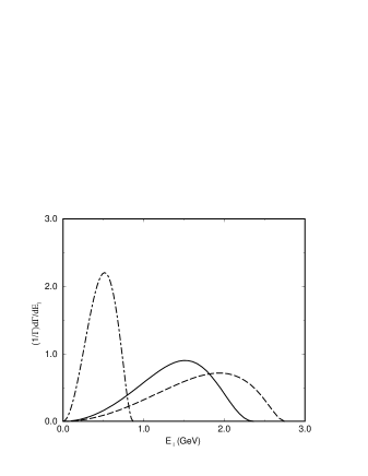
FIG. 14.: Normalized charged lepton energy spectrum for the processes $\Lambda_{c}\rightarrow\Lambda\ell\nu_{\ell}$ (dot-dashed line), $\Lambda_{b}\rightarrow\Lambda_{c}\ell\nu_{\ell}$ (solid line) and $\Lambda_{b}\rightarrow p\ell\nu_{\ell}$ (dashed line).

The knowledge of the form factors also allows us to calculate the charged lepton energy spectrum. In Fig. 14 we plot $(1/\Gamma){d\Gamma}/{dE_{l}}$ versus the energy of the charged lepton, $E_{l}$, for the three studied decays. The spectra have exactly the same shapes for $\kappa=1$ or $2$ and for either the rectangular or triangular region in the continuum model.

5. Summary and Conclusions

We have developed in this paper the complete kinematical formalism to obtain the physical form factors of semileptonic hyperon decays from the off-shell three-point functions and QCD sum rules. We have obtained the $t$ -dependence of the form factors directly from the sum rules in the physical region for positive values of the momentum transfer since, in this case, the cut in the $t$ channel starts at $t\sim m_{Q}^{2}$ ($m_{Q}$ being the heavy quark mass), and thus the Euclidean region stretches up to that threshold. We have applied this formalism to the $\Lambda_{c}^{+}\to\Lambda+e^{+}+\nu_{e}$, $\Lambda_{b}\to\Lambda_{c}+\ell^{-}+\bar{\nu}_{\ell}$ and $\Lambda_{b}\to p+\ell^{-}+\bar{\nu}_{\ell}$ semileptonic decays. It turns out that the sum rule for $\Lambda_{c}^{+}\to\Lambda+e^{+}+\nu_{e}$ depends much more strongly on the values of parameters used in the sum rules than what has been found in the case of the analogous mesonic decay $D\to K^{(*)}+\mbox{ leptons }$. In particular, the dependence on the choice of the model for the continuum makes detailed predictions impossible. This is not surprising since: a) the higher dimension of the baryon currents implies a faster increase of the discontinuities along the cuts and thus a stronger dependence on the assumed onset of duality (continuum threshold); and b) spin leads to further complications. In our projection we have only singled out the ground state with spin 1/2 and put all remaining contributions in the pertubatively treated continuum. For higher spin states, which are also present in the three-point function, the projection is much more involved and such a simple treatment may be less justifiable than in the scalar and vector meson cases. This difficulty reflects itself in a certain inconsistency of the sum rules for the same form factor obtained from different gamma-matrix structures (see Sec. IV and Appendices B and C). We have therefore studied in more detail the $f_{I}f_{F}$ structure (see Eq. (32)). Another special feature of the $\Lambda_{c}$ semileptonic decay is the importance of the four-quark condensate which, for some values of the continuum thresholds, gives much larger contribution than the perturbative part. According to the original SVZ philosophy [1], this brings doubt to the use of the sum rule approach in this case,and, furthermore, we must remark that the value of the four-quark condensate is only poorly known. So it is natural that the present analysis of the $\Lambda_{c}$ decay leads to very large errors, and the same is true, to an even larger extent, for $\Lambda_{b}\to p\ell^{-}\bar{\nu}_{\ell}$.

The situation for $\Lambda_{b}\to\Lambda_{c}\ell^{-}\bar{\nu}_{\ell}$ is much more favorable. Here the symmetries valid in the limit of the masses going to infinity make themselves remarkable also in our treatment of full QCD. The result of the present more complete investigation modifies our earlier assertion [11] about large $1/M^{2}$ corrections for this decay. This is mainly due to the choice of the appropriate continuum model. It has been strongly argued by Blok and Shifman [25] that only a triangular cutoff (see Sec. IV) is adequate for HQET, since a rectangular cutoff does not project out the p-waves properly. This argument becomes much more important for fermions than for mesons, since the change from a rectangular to a triangular cutoff, which had no strong effect on the decay rate of the mesons, is very important for baryons. So we conclude that a treatment of the $\Lambda_{b}\to\Lambda_{c}\ell^{-}\bar{\nu}_{\ell}$ through HQET sum rules is satisfactory. Nevertheless, we must remark that the influence of the continumm threshold on the phenomenologically important slope of the Isgur-Wise function is not negligible also in the HQET limit.

We have calculated the semileptonic decay form factors using sum rules with three different tensor structures. The most robust result that we have obtained for the form factors is that $F_{1}^{A}(t)=-F_{1}^{V}(t)$ for all decays and structures considered. Different structures lead to different relations between $F_{2}^{V}$ and $F_{2}^{A}$. The only possible way to conciliate the three results would be to have $F_{2}^{V}=F_{2}^{A}=0$, which however is a result valid only for the $f_{I}f_{F}$ structure. In the case of the $\Lambda_{b}$ decay, the numerical values obtained for $F_{2}^{V(A)}$ in the $f^{\prime}_{I}f_{F}$ and $f_{i}f^{\prime}_{F}$ structures are very small and, therefore, consistent with zero. However, in the case of the $\Lambda_{c}$ decay, the numerical values obtained for $F_{2}^{V(A)}$ in the $f^{\prime}_{I}f_{F}$ and $f_{I}f^{\prime}_{F}$ cases are not consistent with zero, and this leads to huge variations in the decay rates obtained in the different cases.

For the process $\Lambda_{b}\to\Lambda_{c}\ell\nu_{\ell}$ our results for the decay width are in agreement with the experimental upper limit, and the extrapolation of the form factors to the maximal momentum transfer agrees very well with the HQET prediction.

We have also calculated the charged lepton energy spectrum and it is interesting to remark that the form of the spectrum is not sensitive to the structure used, neither to the model of continuum, neither to the parametrization of the four-quark condensate.

$$F^{V,A}_{i}(s,u,t)=\frac{F_{i}^{V,A}(t)}{(u-M_{\Lambda_{F}}^{2})(s-M_{\Lambda_{I}}^{2})}~{},~{}({\rm with}~{}i=1,2,3)~{},$$ (71)

and using

$$\lambda(s,t,u)=s^{2}+u^{2}+t^{2}-2su-2st-2ut~{},$$

the 24 unknows defined in Eq. (15) are given in term of the traces by

$$F_{1}^{V}(s,u,t)f_{I}f_{F}=\frac{1}{4[\lambda(s,t,u)]^{2}}\cdot$$ (112)

$$\bigg{[}t\lambda(s,u,t)~{}x_{3}+(2s^{2}+2st-t^{2}-4su+2tu+2u^{2})~{}x_{4}$$

$$-3\,t\,\left(s-u\right)~{}x_{5}-3t\left(s-u\right)~{}x_{6}+3t^{2}~{}x_{7}\bigg{]}$$

$$F_{1}^{V}(s,u,t)f_{I}f^{\prime}_{F}=\frac{1}{8[\lambda(s,t,u)]^{2}}\cdot$$

$$\bigg{[}2(s-u)\lambda(s,t,u)~{}x_{1}-2t\lambda(s,t,u)~{}x_{2}-t\lambda(s,t,u)~{}x_{8}+t\lambda(s,t,u)~{}x_{9}$$

$$-\left(2s^{2}-st-t^{2}-4su+5tu+2u^{2}\right)~{}x_{10}+3\,t\,\left(s-t-u\right)~{}x_{11}\bigg{]}$$

$$F_{1}^{V}(s,u,t)f^{\prime}_{I}f_{F}=\frac{1}{8[\lambda(s,t,u)]^{2}}\cdot$$

$$\bigg{[}2(s-u)\lambda(s,t,u)~{}x_{1}-2t\lambda(s,t,u)~{}x_{2}-t\lambda(s,t,u)~{}x_{8}-t\lambda(s,t,u)~{}x_{9}$$

$$+\left(2\,{s^{2}}+5\,s\,t-{t^{2}}-4\,s\,u-t\,u+2u^{2}\right)~{}x_{10}-3\,t\,\left(s+t-u\right)~{}x_{11}\bigg{]}$$

$$F_{1}^{V}(s,u,t)f^{\prime}_{I}f^{\prime}_{F}=\frac{1}{8[\lambda(s,t,u)]^{2}}\cdot$$

$$\bigg{[}-t(s-t+u)\lambda(s,t,u)~{}x_{3}-(s-t+u)~{}(2s^{2}+2st-t^{2}-4su+2tu+2u^{2})~{}x_{4}$$

$$+3\,t\,\left(s-t+u\right)\,\left(s-u\right)~{}x_{5}+\left(s-u\right)\,\left(2\,{s^{2}}-s\,t-{t^{2}}-4\,s\,u-t\,u+2\,{u^{2}}\right)~{}x_{6}$$

$$-t\left(2\,{s^{2}}-s\,t-{t^{2}}-4\,s\,u-t\,u+2\,{u^{2}}\right)~{}{x_{7}}+it\lambda(s,t,u)~{}x_{12}\bigg{]}$$

$$F_{2}^{V}(s,u,t)f_{I}f_{F}=-\frac{1}{4[\lambda(s,t,u)]^{2}}\cdot$$

$$\bigg{[}\lambda(s,u,t)~{}x_{8}-3\,\left(s-u\right)~{}x_{10}+3t~{}x_{11}\bigg{]}$$

$$F_{2}^{V}(s,u,t)f_{I}f^{\prime}_{F}=-\frac{1}{8[\lambda(s,t,u)]^{2}}\cdot$$

$$\bigg{[}(s-t-u)\lambda(s,t,u)~{}x_{3}+\left(4s^{2}-5st+t^{2}+4su+tu-8u^{2}\right)~{}x_{4}$$

$$-\left({s^{2}}+s\,t-2\,{t^{2}}-2\,s\,u+7\,t\,u+{u^{2}}\right)~{}x_{5}-3\,\left(s-t-u\right)\left(s-u\right)~{}x_{6}$$

$$+3\,t\,\left(s-t-u\right)~{}x_{7}-i\lambda(s,t,u)~{}x_{12}\bigg{]}$$

$$F_{2}^{V}(s,u,t)f^{\prime}_{I}f_{F}=-\frac{1}{8[\lambda(s,t,u)]^{2}}\cdot$$

$$\bigg{[}-(s+t-u)\lambda(s,t,u)~{}x_{3}-\left(8s^{2}-st-t^{2}-4su+5tu-4u^{2}\right)~{}x_{4}$$

$$+\left({s^{2}}+7\,s\,t-2\,{t^{2}}-2\,s\,u+t\,u+{u^{2}}\right)~{}x_{5}+3\,\left(s-u\right)\left(s+t-u\right)x_{6}$$

$$-3\,t\,\left(s+t-u\right)~{}x_{7}-i\lambda(s,t,u)~{}x_{12}\bigg{]}$$

$$F_{2}^{V}(s,u,t)f^{\prime}_{I}f^{\prime}_{F}=-\frac{1}{8[\lambda(s,t,u)]^{2}}\cdot$$

$$\bigg{[}-2\left(s-u\right)\lambda(s,t,u)~{}x_{1}+2t\lambda(s,t,u)~{}x_{2}+\left(s+u\right)\lambda(s,t,u)~{}x_{8}$$

$$-\left(s-u\right)\lambda(s,t,u)~{}x_{9}+3\,\left(s-u\right)\,\left(s-t+u\right)~{}x_{10}$$

$$-\left({s^{2}}+s\,t-2\,{t^{2}}-2\,s\,u+t\,u+u^{2}\right)~{}x_{11}\bigg{]}$$

$$F_{3}^{V}(s,u,t)f_{I}f_{F}=\frac{1}{4[\lambda(s,t,u)]^{2}}\cdot$$

$$\bigg{[}\lambda(s,u,t)~{}x_{9}-3\,\left(2\,s-t+2\,u\right)~{}x_{10}+3\,\left(s-u\right)~{}x_{11}\bigg{]}$$

$$F_{3}^{V}(s,u,t)f_{I}f^{\prime}_{F}=\frac{1}{8[\lambda(s,t,u)]^{2}}\cdot$$

$$\bigg{[}(s-t+3u)\lambda(s,t,u)~{}x_{3}+3(2s-t+2u)(s-t+3u)~{}x_{4}$$

$$-3\,\left(s-u\right)\,\left(s-t+3\,u\right)~{}x_{5}-\left(5\,{s^{2}}-7\,s\,t+2\,{t^{2}}+2\,s\,u-t\,u-7\,{u^{2}}\right)~{}x_{6}$$

$$+\left(2\,{s^{2}}-s\,t-{t^{2}}-4\,s\,u+5\,t\,u+2\,{u^{2}}\right)~{}x_{7}-i~{}\lambda(s,t,u)~{}x_{12}\bigg{]}$$

$$F_{3}^{V}(s,u,t)f^{\prime}_{I}f_{F}=\frac{1}{8[\lambda(s,t,u)]^{2}}\cdot$$

$$\bigg{[}-(3s-t+u)\lambda(s,t,u)~{}x_{3}-3(3s-t+u)(2s-t+2u)~{}x_{4}$$

$$+3\,\left(3\,s-t+u\right)\,\left(s-u\right)~{}x_{5}+\left(7\,{s^{2}}+s\,t-2\,{t^{2}}-2\,s\,u+7\,t\,u-5\,{u^{2}}\right)~{}x_{6}$$

$$-\left(2\,{s^{2}}+5\,s\,t-{t^{2}}-4\,s\,u-t\,u+2u^{2}\right)~{}x_{7}+i~{}\lambda(s,t,u)~{}x_{12}\bigg{]}$$

$$F_{3}^{V}(s,u,t)f^{\prime}_{I}f^{\prime}_{F}=\frac{1}{8[\lambda(s,t,u)]^{2}}\cdot$$

$$\bigg{[}-2(2s-t+2u)\lambda(s,t,u)~{}x_{1}+2(s-u)\lambda(s,t,u)~{}x_{2}$$

$$+(s-u)\lambda(s,t,u)~{}x_{8}-(s+u)\lambda(s,t,u)~{}x_{9}$$

$$+\left(5\,{s^{2}}-7\,s\,t+2t^{2}+14su-7tu+5u^{2}\right)~{}x_{10}-3\left(s-t+u\right)\left(s-u\right)~{}x_{11}\bigg{]}$$

and for the axial form factors we obtain

$$F_{1}^{A}(s,u,t)f_{I}f_{F}=\frac{1}{4[\lambda(s,t,u)]^{2}}\cdot$$ (113)

$$\bigg{[}t\lambda(s,t,u)~{}u_{3}+\left(2s^{2}+2st-t^{2}-4su+2tu+2u^{2}\right)~{}u_{4}$$ (114)

$$-3t\left(s-u\right)~{}u_{5}-3\,t\,\left(s-u\right)~{}u_{6}+3t^{2}~{}u_{7}\bigg{]}$$ (115)

$$F_{1}^{A}(s,u,t)f_{I}f^{\prime}_{F}=\frac{1}{8[\lambda(s,t,u)]^{2}}\cdot$$ (116)

$$\bigg{[}-2(s-u)\lambda(s,t,u)~{}u_{1}+2t\lambda(s,t,u)~{}u_{2}+t\lambda(s,t,u)~{}u_{8}-t\lambda(s,t,u)~{}u_{9}$$ (117)

$$+\left(2s^{2}-st-t^{2}-4su+5tu+2u^{2}\right)~{}u_{10}-3\,t\,\left(s-t-u\right)~{}u_{11}\bigg{]}$$ (118)

$$F_{1}^{A}(s,u,t)f^{\prime}_{I}f_{F}=\frac{1}{8[\lambda(s,t,u)]^{2}}\cdot$$ (119)

$$\bigg{[}2\,\left(s-u\right)\lambda(s,t,u)~{}u_{1}-2t\lambda(s,t,u)~{}u_{2}-t\lambda(s,t,u)~{}u_{8}-t\lambda(s,t,u)~{}u_{9}$$ (120)

$$+\left(2s^{2}+5st-t^{2}-4su-tu+2u^{2}\right)~{}u_{10}-3\,t\,\left(s+t-u\right)~{}u_{11}\bigg{]}$$ (121)

$$F_{1}^{A}(s,u,t)f^{\prime}_{I}f^{\prime}_{F}=\frac{1}{8[\lambda(s,t,u)]^{2}}\cdot$$ (122)

$$\bigg{[}t(s-t+u)\lambda(s,t,u)~{}u_{3}+(s-t+u)(2s^{2}+2st-t^{2}-4su+2tu+2u^{2})~{}u_{4}$$ (123)

$$-3\,t\,\left(s-u\right)\,\left(s-t+u\right)\,{u_{5}}-\left(s-u\right)\left(2\,{s^{2}}-s\,t-{t^{2}}-4\,s\,u-t\,u+2\,{u^{2}}\right)\,{u_{6}}$$ (124)

$$+t\left(2s^{2}-st-t^{2}-4su-tu+2u^{2}\right)~{}u_{7}-i\,t\lambda(s,t,u)~{}u_{12}\bigg{]}$$ (125)

$$F_{2}^{A}(s,u,t)f_{I}f_{F}=-\frac{1}{4[\lambda(s,t,u)]^{2}}\cdot$$ (126)

$$\bigg{[}-\lambda(s,t,u)~{}u_{8}+3\,\left(s-u\right)~{}u_{10}-3t~{}u_{11}\bigg{]}$$ (127)

$$F_{2}^{A}(s,u,t)f^{\prime}_{I}f_{F}=-\frac{1}{8[\lambda(s,t,u)]^{2}}\cdot$$ (128)

$$\bigg{[}(s-t-u)\lambda(s,t,u)~{}u_{3}+\left(4s^{2}-5st+t^{2}+4su+tu-8u^{2}\right)~{}u_{4}$$ (129)

$$-\left({s^{2}}+s\,t-2\,{t^{2}}-2\,s\,u+7\,t\,u+{u^{2}}\right)~{}u_{5}-3\,\left(s-u\right)\,\left(s-t-u\right)~{}u_{6}$$ (130)

$$+3t\left(s-t-u\right)~{}u_{7}-i\lambda(s,u,t)~{}u_{12}\bigg{]}$$ (131)

$$F_{2}^{A}(s,u,t)f^{\prime}_{I}f_{F}=-\frac{1}{8[\lambda(s,t,u)]^{2}}\cdot$$ (132)

$$\bigg{[}(s+t-u)\lambda(s,t,u)~{}u_{3}+\left(8s^{2}-st-t^{2}-4su+5tu-4u^{2}\right)~{}u_{4}$$ (133)

$$-\left({s^{2}}+7\,s\,t-2t^{2}-2su+tu+u^{2}\right)~{}u_{5}-3\,\left(s-u\right)\left(s+t-u\right)~{}u_{6}$$ (134)

$$+3\,t\,\left(s+t-u\right)~{}u_{7}+i\lambda(s,u,t)~{}u_{12}\bigg{]}$$ (135)

$$F_{2}^{A}(s,u,t)f^{\prime}_{I}f^{\prime}_{F}=-\frac{1}{8[\lambda(s,t,u)]^{2}}\cdot$$ (136)

$$\bigg{[}-2\,\left(s-u\right)\lambda(s,u,t)~{}u_{1}+2t\lambda(s,t,u)~{}u_{2}+\left(s+u\right)\lambda(s,t,u)~{}u_{8}$$ (137)

$$-\left(s-u\right)\lambda(s,t,u)~{}u_{9}+3\left(s-u\right)\left(s-t+u\right)~{}u_{10}$$ (138)

$$-\left(s^{2}+st-2t^{2}-2su+tu+u^{2}\right)~{}u_{11}\bigg{]}$$ (139)

$$F_{3}^{A}(s,u,t)f_{I}f_{F}=\frac{1}{4[\lambda(s,t,u)]^{2}}\cdot$$ (140)

$$\bigg{[}-\lambda(s,t,u)~{}u_{9}+3\,\left(2\,s-t+2\,u\right)~{}u_{10}-3\,\left(s-u\right)~{}u_{11}\bigg{]}$$ (141)

$$F_{3}^{A}(s,u,t)f_{I}f^{\prime}_{F}=\frac{1}{8[\lambda(s,t,u)]^{2}}\cdot$$ (142)

$$\bigg{[}(s-t+3u)\lambda(s,t,u)~{}u_{3}+3(2s-t+2u)(s-t+3u)~{}u_{4}$$ (143)

$$-3\left(s-t+3\,u\right)\left(s-u\right)~{}u_{5}-\left(5\,{s^{2}}-7\,s\,t+2\,{t^{2}}+2\,s\,u-t\,u-7\,{u^{2}}\right)~{}u_{6}$$ (144)

$$+\left(2s^{2}-st-t^{2}-4su+5tu+2u^{2}\right)~{}u_{7}-i\lambda(s,t,u)~{}u_{12}\bigg{]}$$ (145)

$$F_{3}^{A}(s,u,t)f^{\prime}_{I}f_{F}=\frac{1}{8[\lambda(s,t,u)]^{2}}\cdot$$ (146)

$$\bigg{[}(3s-t+u)\lambda(s,t,u)~{}u_{3}+3(3s-t+u)(2s-t+2u)~{}u_{4}$$ (147)

$$-3\,\left(3\,s-t+u\right)\,\left(s-u\right)~{}u_{5}-\left(7\,{s^{2}}+s\,t-2\,{t^{2}}-2\,s\,u+7\,t\,u-5\,{u^{2}}\right)~{}u_{6}$$ (148)

$$+\left(2s^{2}+5st-t^{2}-4su-tu+2\,{u^{2}}\right)~{}u_{7}-i\lambda(s,t,u)~{}u_{12}\bigg{]}$$ (149)

$$F_{3}^{A}(s,u,t)f^{\prime}_{I}f^{\prime}_{F}=\frac{1}{8[\lambda(s,t,u)]^{2}}\cdot$$ (150)

$$\bigg{[}-2(2s-t+2u)\lambda(s,t,u)~{}u_{1}+2(s-u)\lambda(s,t,u)~{}u_{2}+(s-u)\lambda(s,t,u)~{}u_{8}$$ (151)

$$-(s+u)\lambda(s,t,u)~{}u_{9}+\left(5\,{s^{2}}-7\,s\,t+2\,{t^{2}}+14\,s\,u-7\,t\,u+5\,{u^{2}}\right)~{}u_{10}$$ (152)

$$-3\left(s-t+u\right)\,\left(s-u\right)~{}u_{11}\bigg{]}~{}.$$ (153)

Appendix 2 . Form Factors in the $f^{\prime}_{I}f_{F}$ Structure

For the sum rules based on $f^{\prime}_{I}f_{F}$ structures (see Eq.(15)) we obtain the general results

$$F^{A}_{1}(t)=-\,F^{V}_{1}(t);\;F^{A}_{2}(t)=F^{V}_{2}(t)\;,$$ (154)

and only the perturbative diagram contributes to $F^{V(A)}_{2}$. Since the form factors $F_{3}^{V(A)}$ contribute to the semileptonic decays at ${\cal{O}}(m_{\ell}^{2}/q^{2})$ [16] and are thus difficult to measure, we will not present results for these quantities here.

The stability behavior of the sum rules as a function of the Borel mass is here very similar to that shown in Figs. 7,9 and 12, and the pole fits also describe very well the $t$-dependence of the form factors (as well as the curves shown in Figs. 8,10 and 13). In Table IV we give the pole parametrization of the form factors for the process $\Lambda_{b}\to\Lambda_{c}\ell\nu_{\ell}$ for two values of $\kappa$ (see Eq. (29)) and for the two forms of regions of continuum contribution considered. The other parameters are exactly the same as discussed in section IV. The continuum thresholds are obtained using method 1 for $\Lambda_{b}$ and $\Lambda_{c}$, and method 2 for $\Lambda$.

Table IV

Pole parametrization of the form factors for the process $\Lambda_{b}\to\Lambda_{c}\ell\nu_{\ell}$ for different values of the parameters and choices of continuum model.

continuum model	$\;\kappa\;$	$\;F_{1}^{V}(t)\;$	$F_{2}^{V}(t)(\nobreak\,\mbox{GeV}^{-1})$
rectangular	1	${7.73/(17.79-t)}$	${-0.20/(13.51-t)}$
rectangular	2	${8.93/(18.70-t)}$	${-0.22/(14.91-t)}$
triangular	1	${16.60/(24.24-t)}$	${-0.55/(18.63-t)}$
triangular	2	${19.02/(25.64-t)}$	${-0.61/(19.10-t)}$

We can see from Eq. (47) that the IW function at ${\cal{O}}(1/m)$ is given by $G_{1}^{A}=-F_{1}^{A}-(M_{\Lambda_{F}}-M_{\Lambda_{I}})F_{2}^{A}$. The extrapolation of the fits given in Table IV to the maximal momentum transfer value yields $G_{1}^{A}(t_{\rm max})=1.0~{}(0.93)$ for $\kappa=2~{}(1)$ for the rectangular region, and $G_{1}^{A}(t_{\rm max})=1.04~{}(1.03)$ for $\kappa=2~{}(1)$ for the triangular region, in very good agreement with the HQET prediction.

With the pole parametrizations given above, the $\Lambda_{b}\rightarrow\Lambda_{c}\ell\nu_{\ell}$ decay rate is

$$\Gamma(\Lambda_{b}\to\Lambda_{c}\ell^{-}\bar{\nu}_{\ell})=(5.1\pm 1.8)\times 10^{-14}\;{\rm GeV}~{},$$ (155)

where the errors reflect variations of $\kappa$ from 1 to 2 and the different choices for the continuum contribution. This value is larger than the one obtained based on $f_{I}$ and $f_{F}$ structures (see Eq. (64)), but it is still in agreement with other predictions [16, 27, 28, 29] and with the experimental upper limit [30] (see Eq. (65)).

In the case of the process $\Lambda_{c}\rightarrow\Lambda\ell\nu_{\ell}$, when the form factors are extracted from the sum rules based on $f^{\prime}_{I}f_{F}$ structure, we obtain a very large decay rate

$$\Gamma(\Lambda_{c}^{+}\to\Lambda+e^{+}+\nu_{e})=(19\pm 5)\times 10^{-14}\;{\rm GeV}~{},$$ (156)

which is much larger than the experimental value[30] (see Eq. (65)) and more than two times larger than the value obtained using the sum rules based on $f_{I}f_{F}$ structure (see Eq. (68)). The mathematical reason for this discrepancy is that while the $F_{1}^{V(A)}$ form factors extracted from both $f_{I}f_{F}$ and $f^{\prime}_{I}f_{F}$ structures are in very good agreement with each other, this is not the case for the $F_{2}^{V(A)}$ form factors, which are zero when the $f_{I}f_{F}$ structure is used and of about $-0.1(-0.2)$ (for $\kappa=1(2)$) at $t=0$ for the $f^{\prime}_{I}f_{F}$ structure. This can be seen in Table V, where we give the pole parametrization of the form factors for the process $\Lambda_{c}\to\Lambda\ell\nu_{\ell}$ extracted from the sum rules based on the $f^{\prime}_{I}f_{F}$ structure.

Table V

Pole parametrization of the form factors for the process $\Lambda_{c}\to\Lambda\ell\nu_{\ell}$ for different values of the parameters and choices of the continuum model.

continuum model	$\;\kappa\;$	$\;F_{1}^{V}(t)\;$	$F_{2}^{V}(t)(\nobreak\,\mbox{GeV}^{-1})$
rectangular	1	${1.46/(2.98-t)}$	${-0.19/(1.80-t)}$
rectangular	2	${1.78/(3.52-t)}$	${-0.21/(1.94-t)}$
triangular	1	${2.80/(4.10-t)}$	${-0.55/(2.84-t)}$
triangular	2	${3.06/(4.59-t)}$	${-0.53/(3.00-t)}$

The contribution of $F_{2}^{V(A)}$ is responsible for the strong differences in the results for the calculated decay rates. In the $\Lambda_{b}\rightarrow\Lambda_{c}\ell\nu_{\ell}$ case, an inspection of Tables IV and V shows that although the $F_{1}^{V(A)}$ form factors are of the same order of magnitude in the $\Lambda_{b}$ and $\Lambda_{c}$ decays, the $F_{2}^{V(A)}$ form factors are one order of magnitude larger in the $\Lambda_{c}$ decay than in the $\Lambda_{b}$ decay. The results for the $\Lambda_{b}$ decay did not change much because the values of the form factors $F_{2}^{V(A)}$ are consistent with zero for both $f_{I}f_{F}$ and $f^{\prime}_{I}f_{F}$ structures.

Appendix 3 . Form Factors in the $f_{I}f^{\prime}_{F}$ Structure

The observed discrepancy in the results for $F_{2}^{V(A)}$ form factors comparing the $f_{I}f_{F}$ and $f^{\prime}_{I}f_{F}$ structures for the $\Lambda_{c}\to\Lambda\ell\nu_{\ell}$ process described above leads us now to consider the form factors obtained through the $f_{I}f^{\prime}_{F}$ structure. For these sum rules we obtain

$$F^{A}_{1}(t)=-\,F^{V}_{1}(t);\;F^{A}_{2}(t)=-F^{V}_{2}(t)\;.$$ (157)

Comparing Eq. (157) with Eq. (154) we see that the general results are correct only if $F_{2}^{V(A)}=0$, which is true only for the $f_{I}f_{F}$ structure. Therefore, we can foresee more discrepancies here. For the $F_{1}$ form factor, this structure gives a result about 30% smaller than in the previous studied structures for the $\Lambda_{b}$ decay, but gives a result with a factor more than two smaller for the $\Lambda_{c}$ decay. Moreover, while it is still possible to parametrize the $t$-dependence of $F_{1}$ with a monopole form in the case of the $\Lambda_{b}$ decay (with an agreement similar to the other structures), this is not possible for the $\Lambda_{c}$ decay. The pole mass needed to fit the $t$ behavior is smaller than $t_{\rm max}=(M_{\Lambda_{c}}-M_{\Lambda})^{2}$. We have used an exponential form factor of the type $\exp{(t-a)/b}$ to fit the $t$-dependence of $F_{1}$, but the agreement is rather poor.

For the $F_{2}$ form factor a monopole fit is possible for both decays, and its magnitude is about 20% smaller than for the structure $f^{\prime}_{I}f_{F}$ for the $\Lambda_{b}$ decay (therefore, consistent with zero), and a factor more than two smaller for the $\Lambda_{c}$ decay.

In Table VI we give the pole parametrization of the form factors for the two processes $\Lambda_{b}\to\Lambda_{c}\ell\nu_{\ell}$ and $\Lambda_{c}\to\Lambda\ell\nu_{\ell}$, extracted from the sum rules based on the $f_{I}f^{\prime}_{F}$ structure.

Table VI

Parametrization of the form factors for the processes $\Lambda_{b}\to\Lambda_{c}\ell\nu_{\ell}$ and $\Lambda_{c}\to\Lambda\ell\nu_{\ell}$ for different values of the parameters and continuum models.

		$\Lambda_{b}\to\Lambda_{c}\ell\nu_{\ell}$		$\Lambda_{c}\to\Lambda\ell\nu_{\ell}$
continuum model	$\;\kappa\;$	$\;F_{1}^{V}(t)\;$	$F_{2}^{V}(t)(\nobreak\,\mbox{GeV}^{-1})$	$\;F_{1}^{V}(t)\;$	$F_{2}^{V}(t)(\nobreak\,\mbox{GeV}^{-1})$
rectangular	1	${6.66/(20.27-t)}$	${-0.21/(15.15-t)}$	$e^{(t-2.07)/0.95}$	${-0.15/(2.85-t)}$
rectangular	2	${8.13/(22.50-t)}$	${-0.22/(13.63-t)}$	$e^{(t-2.08)/0.97}$	${-0.17/(3.38-t)}$
triangular	1	${13.74/(26.68-t)}$	${-0.41/(18.65-t)}$	$e^{(t-2.03)/1.09}$	${-0.18/(2.79-t)}$
triangular	2	${16.17/(29.12-t)}$	${-0.45/(19.04-t)}$	$e^{(t-1.72)/1.02}$	${-0.20/(3.05-t)}$

With the above parametrizations we obtain for the the decay rates

$$\Gamma(\Lambda_{b}\to\Lambda_{c}\ell^{-}\bar{\nu}_{\ell})=(1.8\pm 0.8)\times 10^{-14}\;{\rm GeV},$$ (158)

and

$$\Gamma(\Lambda_{c}^{+}\to\Lambda+e^{+}+\nu_{e})=(2\pm 1)\times 10^{-14}\;{\rm GeV}.$$ (159)

Therefore, the sum rules based on the structure $f_{I}f^{\prime}_{F}$ give too small decay rates for both $\Lambda_{b}$ and $\Lambda_{c}$ decays. Of course the variation in the three structures considered is much larger in the case of the $\Lambda_{c}$ decay and this should be expected since the simple current used is not the best suited to describe $\Lambda$, as can be seen by the short-dashed line in Fig. 11, which shows that the 1 structure is not trustworth in the mass sum rule, and this structure is related with the $f^{\prime}$ structure in the decay.

It is important to mention that even with this structure the extrapolation of the fits given in Table VI to the maximal momentum transfer in the $\Lambda_{b}$ decay yields for the IW function the value $G_{1}^{A}(t_{\rm max})=0.97\pm 0.04$ (where $G_{1}^{A}=-F_{1}^{A}-(M_{\Lambda_{F}}-M_{\Lambda_{I}})F_{2}^{A}$), in very good agreement with the HQET prediction.

REFERENCES

- [1] M.A. Shifman, A.I. Vainshtein and V.I. Zakharov, Nucl. Phys. B147, 385 (1979); B147, 448 (1979).
- [2] S. Narison, QCD Spectral Sum Rules , World Scientific, Singapore 1989.
- [3] M.A. Shifman, Vacuum Structure and QCD Sum Rules, North Holland, Amsterdam 1992.
- [4] E.V. Shuryak, Nucl. Phys. B198, 83 (1982).
- [5] M.B. Voloshin and M.A. Shifman, Sov. J. Nucl. Phys. 45, 292 (1987); 47,511 (1988).
- [6] S. Nussinov and W. Wetzel, Phys. Rev D 36, 130 (1987).
- [7] N. Isgur and M.B. Wise, Phys. Lett. B237, 527 (1990); Nucl. Phys. B348, 276 (1991).
- [8] H. Georgi, Phys. Lett. B240, 447 (1990); Nucl. Phys. B348, 293 (1991).
- [9] T. Mannel, W. Roberts and Z. Ryzak, Nucl. Phys. B355, 38 (1991).
- [10] M. Neubert, Phys. Rep. 245, 259 (1994).
- [11] H.G. Dosch, E. Ferreira, M. Nielsen and R. Rosenfeld, Phys. Lett. B431, 173 (1998).
- [12] P. Ball, V.M. Braun and H.G. Dosch, Phys. Rev. D44, 3567 (1991).
- [13] M. Neubert, Theory of Beauty Lifetimes, Second International Conference on B Physics and CP Violation, Honolulu 1997, hep-ph/9707217.
- [14] B.L. Ioffe and A.V. Smilga, Phys. Lett. B114, 353 (1982); Nucl. Phys. B216, 373 (1993).
- [15] V.A. Nesterenko and A.V. Radyushkin, Phys. Lett. B115, 410 (1982).
- [16] J.G. Körner, M. Krämer and D. Pirjol, Prog. Part. Nucl. Phys. 33 , 787 (1994).
- [17] B.L. Ioffe, Nucl. Phys. B188, 317 (1981); Erratum: B191, 591 (1981).
- [18] Y. Chung, et al. Nucl. Phys. B197, 55 (1982).
- [19] E. Bagan, M. Chabab, H.G. Dosch and S. Narison, Phys. Lett. B278, 367 (1992); B287, 176 (1992); B301, 243 (1993).
- [20] E. Bagan, P. Ball and P. Gosdzinsky, Phys. Lett B301, 249 (1993).
- [21] A.G. Grozin, O.I. Yakovlev, Phys. Lett. B291, 441 (1992).
- [22] Y-b. Dai et al Phys. Lett. B387, 379 (1996).
- [23] M.E. Luke, Phys. Lett. B252, 447 (1990).
- [24] M. Neubert, Phys. Rev. D45, 2451 (1992).
- [25] B.Blok, M.A. Shifman, Phys. Rev. D47, 2949 (1993).
- [26] M. Neubert, Phys. Lett. B338, 84 (1994).
- [27] M. A. Ivanov, V. E. Lyubovitskij, J. G. Körner and P. Kroll, Phys. Rev. D56, 348 (1997).
- [28] Y. Dai, C. Huang, M. Huang and C. Liu, Phys. Lett. B387, 379 (1996).
- [29] J.-P. Lee, C. Liu and H.S. Song, Phys. Rev. D58, 14 (1998).
- [30] Particle Data Group, Eur. Phys. Jour. C3, 1 (1998).
- [31] N. Stella for the UKQCD coll., Nucl. Phys. Proc. Suppl. 53, 408 (1997).
- [32] M.B. Gavela, Phys. Lett. B83, 367 (1979).
- [33] R. Pérez-Marcial et al., Phys. Rev. D40, 2955 (1989).
- [34] R. Singleton, Phys. Rev. D43, 2939 (1991).
- [35] H.-Y. Cheng and B. Tseng, Phys. Rev. D53, 1457 (1996).
- [36] C.-S. Huang, C.-F. Qiao and H.-G. Yan, Phys. Lett. B437, 403 (1998).
- [37] P. Ball, V.M. Braun, Phys. Rev. D55, 5561 (1997).