UAB-FT-452 February, 1999 hep-ph/9903213

$\Gamma(H^{+}\to t\bar{b})$ in the MSSM: a handle for SUSY charged Higgs at the Tevatron and the LHC

J.A. COARASA, Jaume GUASCH, Joan SOLÀ

Grup de Física Teòrica

and

Institut de Física d’Altes Energies

Universitat Autònoma de Barcelona

08193 Bellaterra (Barcelona), Catalonia, Spain

ABSTRACT

We compute $\Gamma({H^{+}\to t\bar{b}})$ at one-loop in the MSSM and show how future data at the Tevatron and/or at the LHC could be used to unravel the potential SUSY nature of the charged Higgs.

1 Introduction

The charged Higgs boson can decay hadronically into several quark final states, and if it is sufficiently heavy it would dominantly decay into top and bottom quarks. We will compute the effects of the leading electroweak corrections ($\widetilde{\mathrm{EW}}$) originating from large Yukawa couplings within the MSSM [1] as well as the SUSY-QCD ($\widetilde{\mathrm{QCD}}$) quantum effects mediated by squarks and gluinos and shall compare them with the standard QCD corrections.

The vertex $H^{+}t\bar{b}$ is important not only for the decay under consideration but also in the production mechanism of the charged Higgs. Its associated production with a top quark would contribute to the cross-section for single top-quark production, whose measurement is one of the main goals at the next Tevatron run (Run II).

The relevant Yukawa couplings of the charged Higgs boson with top and bottom quarks:

$$\lambda_{t}\equiv{h_{t}\over g}={m_{t}\over\sqrt{2}\,M_{W}\,\sin{\beta}}\;\;\;\;\;,\;\;\;\;\;\lambda_{b}\equiv{h_{b}\over g}={m_{b}\over\sqrt{2}\,M_{W}\,\cos{\beta}}\,,$$ (1)

are of comparable size within the interval relevant for the Higgs decay

$$20\stackrel{{\scriptstyle\scriptstyle<}}{{{}_{\sim}}}\tan\beta\stackrel{{\scriptstyle\scriptstyle<}}{{{}_{\sim}}}50\,.$$ (2)

2 One-loop Corrected $\Gamma({H^{+}\to t\bar{b}})$ in the MSSM

The interaction lagrangian describing the $H^{+}\,t\,\bar{b}$-vertex in the MSSM is:

$${\cal L}_{Htb}={g\over\sqrt{2}M_{W}}\,H^{+}\,\bar{t}\,[m_{t}\cot\beta\,P_{L}+m_{b}\tan\beta\,P_{R}]\,b+{\rm h.c.}\,,$$ (3)

where $P_{L,R}=1/2(1\mp\gamma_{5})$ are the chiral projector operators. From this the counterterm Lagrangian can be obtained and reads:

$$\delta{\cal L}_{Hbt}={g\over\sqrt{2}\,M_{W}}\,H^{+}\,\bar{t}\left[\delta G_{L}\ m_{t}\,\cot\beta\,\,P_{L}+\delta G_{R}\ m_{b}\,\tan\beta\,P_{R}\right]\,b+{\rm h.c.}\,,$$ (4)

with

$$\delta G_{L} = {\delta m_{t}\over m_{t}}-{\delta v\over v}+\frac{1}{2}\,\delta Z_{H^{+}}+\frac{1}{2}\,\delta Z_{L}^{b}+\frac{1}{2}\,\delta Z_{R}^{t}-{\delta\tan\beta\over\tan\beta}+\delta Z_{HW}\,\tan\beta\,,$$

$$\delta G_{R} = {\delta m_{b}\over m_{b}}-{\delta v\over v}+\frac{1}{2}\,\delta Z_{H^{+}}+\frac{1}{2}\,\delta Z_{L}^{t}+\frac{1}{2}\,\delta Z_{R}^{b}+{\delta\tan\beta\over\tan\beta}-\delta Z_{HW}\,\cot\beta\,,$$

and where $\delta v$ is the counterterm for $v=\sqrt{v_{1}^{2}+v_{2}^{2}}=\sqrt{2}M_{w}/g$, $\delta Z_{H}$ and $\delta Z_{HW}$ stand respectively for the charged Higgs and mixed $H-W$ wave-function. The remaining are the standard wave-function and mass renormalization counterterms for the fermion external lines.

To fix the $\tan\beta$ counterterm we define $\tan\beta$ through $\Gamma({H^{+}\to\tau^{+}\nu_{\tau}})$. Therefore the corrections to this decay are cancelled by suitable counterterms. From this condition and parametrizing the different contributions at one loop to $H^{+}\to t\bar{b}$ in terms of two form factors $H_{L}$, $H_{R}$ the one-loop corrected $H^{+}\to t\bar{b}$ vertex in the MSSM is:

$$\Lambda={i\,g\over\sqrt{2}\,M_{W}}\,\left[m_{t}\,\cot\beta\,(1+G_{L})\,P_{L}+m_{b}\,\tan\beta\,(1+\Lambda_{R})\,P_{R}\right]\,,$$ (5)

where

$$G_{L} = H_{R}+{\delta m_{t}\over m_{t}}+\frac{1}{2}\,\delta Z_{L}^{b}+\frac{1}{2}\,\delta Z_{R}^{t}-\Delta_{\tau}$$

$$- {\delta v^{2}\over v^{2}}+\delta Z_{H^{+}}+(\tan\beta-\cot\beta)\,\delta Z_{HW}\,,$$

$$G_{R} = H_{L}+{\delta m_{b}\over m_{b}}+\frac{1}{2}\,\delta Z_{L}^{t}+\frac{1}{2}\,\delta Z_{R}^{b}+\Delta_{\tau}\,,$$ (6)

and $\Delta_{\tau}$ is a $H^{+}\to\tau^{+}\nu_{\tau}$ process dependent contribution coming from our $\tan\beta$ definition condition.

In the following we will describe the relevant electroweak one-loop supersymmetric diagrams entering the amplitude of $H^{+}\to t\bar{b}$ in the MSSM. At one-loop, we have the diagrams exhibited in Figs. 1-2 apart from the ones entering the calculation of the different counterterms [2]. The computation of the one-loop diagrams requires to use the full structure of the MSSM [1] Lagrangian. The explicit form of the most relevant pieces of this Lagrangian, together with the necessary SUSY notation, is provided in the Appendix.

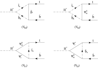
Figure 1: Feynman diagrams, up to one-loop order, for the QCD and electroweak SUSY vertex corrections to the decay process $H^{+}\to t\bar{b}$. Each one-loop diagram is summed over all possible values of the mass-eigenstate gluinos ($\tilde{g}_{r}\,;r=1,\ldots,8$), charginos ($\Psi^{\pm}_{i}\,;i=1,2$), neutralinos ($\Psi^{0}_{\alpha}\,;\alpha=1,...,4$), stop and sbottom squarks ($\tilde{b}_{a},\tilde{t}_{b}\,;a,b=1,2$).

2.1 SUSY vertex diagrams

Following the labelling in Fig. 1 we find the form factors $H_{L}$, $H_{R}$.

• Diagram $(V_{S0})$: Using the convention that lower indices are summed over, whereas upper indices are just for notational convenience one finds:

  $$H_{L} =8\pi\alpha_{s}\,iC_{F}\displaystyle{\frac{G_{ab}^{*}}{m_{t}\cot\beta}} [R^{(t)}_{1b}R^{(b)*}_{1a}(C_{11}-C_{12})m_{t}+R^{(t)}_{2b}R^{(b)*}_{2a}C_{12}m_{b}$$

  $$+R^{(t)}_{2b}R^{(b*)}_{1a}C_{0}m_{\tilde{g}}]\,,$$

  $$H_{R} =8\pi\alpha_{s}\,iC_{F}\displaystyle{\frac{G_{ab}^{*}}{m_{b}\tan\beta}} [R^{(t)}_{2b}R^{(b)*}_{2a}(C_{11}-C_{12})m_{t}+R^{(t)}_{1b}R^{(b)*}_{1a}C_{12}m_{b}$$ (7)

  $$+R^{(t)}_{1b}R^{(b)*}_{2a}C_{0}m_{\tilde{g}}]\,,$$

  where the various $3$-point functions are as in ref. [2], so that, in eq. (7) the C-functions must be evaluated with arguments:

  $$C_{*}=C_{*}\left(p,p^{\prime},m_{\tilde{g}},m_{\tilde{t}_{b}},m_{\tilde{b}_{a}}\right)\,,$$

  and $C_{F}=(N_{C}^{2}-1)/2N_{C}=4/3$ is the colour factor.

• Diagram $(V_{S1})$: Making use of the coupling matrices of eqs. (28) and (33) we introduce the shorthands

  $$A_{\pm}\equiv A_{\pm ai}^{(t)}\ \ \mbox{and}\ \ A_{\pm}^{(0)}\equiv A_{\pm a\alpha}^{(t)}\,,$$

  and define the combinations (omitting indices also for $Q_{\alpha i}^{L},Q_{\alpha i}^{R}$)

  $$A^{(1)}=\cos\!\beta A_{+}^{*}Q^{L}A_{-}^{(0)}\,, E^{(1)}=\cos\!\beta A_{-}^{*}Q^{L}A_{-}^{(0)}\,,$$

  $$B^{(1)}=\cos\!\beta A_{+}^{*}Q^{L}A_{+}^{(0)}\,, F^{(1)}=\cos\!\beta A_{-}^{*}Q^{L}A_{+}^{(0)}\,,$$

  $$C^{(1)}=\sin\!\beta A_{+}^{*}Q^{R}A_{-}^{(0)}\,, G^{(1)}=\sin\!\beta A_{-}^{*}Q^{R}A_{-}^{(0)}\,,$$

  $$D^{(1)}=\sin\!\beta A_{+}^{*}Q^{R}A_{+}^{(0)}\,, H^{(1)}=\sin\!\beta A_{-}^{*}Q^{R}A_{+}^{(0)}\,.$$ (8)

  The contribution from diagram $(V_{S1})$ to the form factors $H_{R}$ and $H_{L}$ is:

  $$H_{R} = M_{L}\left[H^{(1)}\tilde{C}_{0}+\right.$$

  $$+ m_{b}\,\left(m_{t}A^{(1)}+M^{0}_{\alpha}B^{(1)}+m_{b}H^{(1)}+M_{i}D^{(1)}\right)C_{12}$$

  $$+ m_{t}\,\left(m_{t}H^{(1)}+M^{0}_{\alpha}G^{(1)}+m_{b}A^{(1)}+M_{i}E^{(1)}\right)\left(C_{11}-C_{12}\right)$$

  $$+ \left.\left(m_{t}m_{b}A^{(1)}+m_{t}M_{i}E^{(1)}+M^{0}_{\alpha}m_{b}B^{(1)}+M_{i}M^{0}_{\alpha}F^{(1)}\right)C_{0}\right]\,,$$

  $$H_{L} = M_{R}\left[A^{(1)}\tilde{C}_{0}+\right.$$

  $$+ m_{b}\,\left(m_{t}H^{(1)}+M^{0}_{\alpha}G^{(1)}+m_{b}A^{(1)}+M_{i}E^{(1)}\right)C_{12}$$

  $$+ m_{t}\,\left(m_{t}A^{(1)}+M^{0}_{\alpha}B^{(1)}+m_{b}H^{(1)}+M_{i}D^{(1)}\right)\left(C_{11}-C_{12}\right)$$

  $$+ \!\!\!\!\left.\left(m_{t}m_{b}H^{(1)}+m_{t}M_{i}D^{(1)}+M^{0}_{\alpha}m_{b}G^{(1)}+M_{i}M^{0}_{\alpha}C^{(1)}\right)C_{0}\right],$$ (9)

  where the overall coefficients $M_{L}$ and $M_{R}$ are:

  $$M_{L}=-\frac{ig^{2}M_{W}}{m_{b}\tan\beta}\ \ \ \ M_{R}=-\frac{ig^{2}M_{W}}{m_{t}\cot\!\beta}\,.$$ (10)

  In eq. (• ‣ 2.1) the C-functions must be evaluated with arguments:

  $$C_{*}=C_{*}\left(p,p^{\prime},m_{{\tilde{t}}_{a}},M^{0}_{\alpha},M_{i}\right)\,.$$ (11)

• Diagram $(V_{S2})$: For this finite diagram we use the matrices on eqs. (28) and (31), and introduce the shorthands

  $$A_{\pm}^{(b)}\equiv A_{\pm b\alpha}^{(b)}\ \ \mbox{and}\ \ A_{\pm}^{(t)}\equiv A_{\pm a\alpha}^{(t)}\,,$$

  to define the products of coupling matrices

  $$A^{(2)}=G_{ba}A_{+}^{(b)*}A_{-}^{(t)}\,, C^{(2)}=G_{ba}A_{-}^{(b)*}A_{-}^{(t)}\,,$$

  $$B^{(2)}=G_{ba}A_{+}^{(b)*}A_{+}^{(t)}\,, D^{(2)}=G_{ba}A_{-}^{(b)*}A_{+}^{(t)}\,.$$

  The contribution to the form factors $H_{R}$ and $H_{L}$ from this diagram is

  $$H_{R} = \frac{M_{L}}{2M_{W}}\left[m_{b}B^{(2)}C_{12}+m_{t}C^{(2)}\left(C_{11}-C_{12}\right)-M^{0}_{\alpha}D^{(2)}C_{0}\right]\,,$$

  $$H_{L} = \frac{M_{R}}{2M_{W}}\left[m_{b}C^{(2)}C_{12}+m_{t}B^{(2)}\left(C_{11}-C_{12}\right)-M^{0}_{\alpha}A^{(2)}C_{0}\right]\,,$$

  the coefficients $M_{L}$, $M_{R}$ being those of eq. (10) and

  $$C_{*}=C_{*}\left(p,p^{\prime},M^{0}_{\alpha},m_{{\tilde{t}}_{a}},m_{{\tilde{b}}_{b}}\right)\,.$$

• Diagram $(V_{S3})$: For this diagram we will need

  $$A_{\pm}\equiv A_{\pm ai}^{(b)}\ \ \mbox{and}\ \ A_{\pm}^{(0)}\equiv A_{\pm a\alpha}^{(b)}\,,$$

  and again omitting indices we shall use

  $$A^{(3)}=\cos\!\beta A_{+}^{(0)*}Q^{L}A_{-}\,, E^{(3)}=\cos\!\beta A_{-}^{(0)*}Q^{L}A_{-}\,,$$

  $$B^{(3)}=\cos\!\beta A_{+}^{(0)*}Q^{L}A_{+}\,, F^{(3)}=\cos\!\beta A_{-}^{(0)*}Q^{L}A_{+}\,,$$

  $$C^{(3)}=\sin\!\beta A_{+}^{(0)*}Q^{R}A_{-}\,, G^{(3)}=\sin\!\beta A_{-}^{(0)*}Q^{R}A_{-}\,,$$

  $$D^{(3)}=\sin\!\beta A_{+}^{(0)*}Q^{R}A_{+}\,, H^{(3)}=\sin\!\beta A_{-}^{(0)*}Q^{R}A_{+}\,.$$ (12)

  From these definitions the contribution of diagram $(V_{S3})$ to the form factors can be obtained by performing the following changes in that of diagram $(V_{S1})$, eq. (• ‣ 2.1):

  • Everywhere in eqs. (• ‣ 2.1) and (11) replace $M_{i}\leftrightarrow M^{0}_{\alpha}$ and $m_{{\tilde{t}}_{a}}\leftrightarrow m_{{\tilde{b}}_{a}}$.

  • Replace in eq. (• ‣ 2.1) couplings from (• ‣ 2.1) with those of (• ‣ 2.1).

  • Include a global minus sign.

2.2 Higgs vertex diagrams

For the contributions arising from the exchange of virtual Higgs particles and Goldstone bosons in the Feynman gauge, Fig. 2, we write the formula for the form factors by giving the value of the overall coefficient $N$ and the arguments of the corresponding $3$-point functions.

• Diagram $(V_{H1})$:

  $$H_{R} = N\,[m_{b}^{2}(C_{12}-C_{0})+m_{t}^{2}\cot^{2}\!\beta(C_{11}-C_{12})]\,,$$

  $$H_{L} = Nm_{b}^{2}[C_{12}-C_{0}+\tan^{2}\!\beta(C_{11}-C_{12})]\,,$$

  $$N = \mp\frac{ig^{2}}{2}\left(1-\frac{\{M^{2}_{H^{0}},M^{2}_{h^{0}}\}}{2M^{2}_{W}}\right)\frac{\{\cos\!\alpha,\sin\!\alpha\}}{\cos\!\beta}\{{\scriptstyle{\cos\!(\beta-\alpha),\sin\!(\beta-\alpha)}}\}\,,$$

  $$C_{*} = C_{*}\left(p,p^{\prime},m_{b},M_{H^{\pm}},\{M_{H^{0}},M_{h^{0}}\}\right)\,.$$

  

  Figure 2: Feynman diagrams, up to one-loop order, for the Higgs and Goldstone boson vertex corrections to the decay process $H^{+}\to t\bar{b}$.

• Diagram $(V_{H2})$:

  $$H_{R} = N\cot\!\beta[m_{t}^{2}(C_{11}-C_{12})+m_{b}^{2}(C_{0}-C_{12})]\,,$$

  $$H_{L} = Nm_{b}^{2}\tan\beta(2C_{12}-C_{11}-C_{0})\,,$$

  $$N = \frac{ig^{2}}{4}\frac{\{\cos\!\alpha,\sin\!\alpha\}}{\cos\!\beta}\{{\scriptstyle{\sin\!(\beta-\alpha),\cos\!(\beta-\alpha)}}\}\left(\frac{M^{2}_{H^{\pm}}}{M^{2}_{W}}-\frac{\{M^{2}_{H^{0}},M^{2}_{h^{0}}\}}{M^{2}_{W}}\right)\,,$$

  $$C_{*} = C_{*}\left(p,p^{\prime},m_{b},M_{W},\{M_{H^{0}},M_{h^{0}}\}\right)\,.$$

• Diagram $(V_{H3})$:

  $$H_{R} = Nm_{t}^{2}[\cot^{2}\!\beta C_{12}+C_{11}-C_{12}-C_{0}]\,,$$

  $$H_{L} = N\,[m_{b}^{2}\tan^{2}\!\beta C_{12}+m_{t}^{2}(C_{11}-C_{12}-C_{0})]\,,$$

  $$N = -\frac{ig^{2}}{2}\frac{\{\sin\!\alpha,\cos\!\alpha\}}{\sin\!\beta}\{{\scriptstyle{\cos\!(\beta-\alpha),\sin\!(\beta-\alpha)}}\}\left(1-\frac{\{M^{2}_{H^{0}},M^{2}_{h^{0}}\}}{2M^{2}_{W}}\right)\,,$$

  $$C_{*} = C_{*}\left(p,p^{\prime},m_{t},\{M_{H^{0}},M_{h^{0}}\},M_{H^{\pm}}\right)\,.$$

• Diagram $(V_{H4})$:

  $$H_{R} = Nm_{t}^{2}(2C_{12}-C_{11}+C_{0})\cot\!\beta\,,$$

  $$H_{L} = N\,[-m_{b}^{2}C_{12}+m_{t}^{2}(C_{11}-C_{12}-C_{0})]\tan\beta\,,$$

  $$N = \mp\frac{ig^{2}}{4}\frac{\{\sin\!\alpha,\cos\!\alpha\}}{\sin\!\beta}\{{\scriptstyle{\sin\!(\beta-\alpha),\cos\!(\beta-\alpha)}}\}\left(\frac{M^{2}_{H^{\pm}}}{M^{2}_{W}}-\frac{\{M^{2}_{H^{0}},M^{2}_{h^{0}}\}}{M^{2}_{W}}\right)\,,$$

  $$C_{*} = C_{*}\left(p,p^{\prime},m_{t},\{M_{H^{0}},M_{h^{0}}\},M_{W}\right)\,.$$

• Diagram $(V_{H5})$:

  $$H_{R} = N\,[m_{b}^{2}(C_{12}+C_{0})+m_{t}^{2}(C_{11}-C_{12})]\,,$$

  $$H_{L} = Nm_{b}^{2}\tan^{2}\!\beta(C_{11}+C_{0})\,,$$

  $$N = -\frac{ig^{2}}{4}\left(\frac{M^{2}_{H^{\pm}}}{M^{2}_{W}}-\frac{M^{2}_{A^{0}}}{M^{2}_{W}}\right)\,,\,\,\,C_{*}=C_{*}\left(p,p^{\prime},m_{b},M_{W},M_{A^{0}}\right)\,.$$

• Diagram $(V_{H6})$:

  $$H_{R} = Nm_{t}^{2}\cot^{2}\!\beta(C_{11}+C_{0})\,,$$

  $$H_{L} = N\,[m_{b}^{2}C_{12}+m_{t}^{2}(C_{11}-C_{12}+C_{0})]\,,$$

  $$N = -\frac{ig^{2}}{4}\left(\frac{M^{2}_{H^{\pm}}}{M^{2}_{W}}-\frac{M^{2}_{A^{0}}}{M^{2}_{W}}\right)\,,\,\,\,C_{*}=C_{*}\left(p,p^{\prime},m_{t},M_{A^{0}},M_{W}\right)\,.$$

• Diagram $(V_{H7})$:

  $$H_{R} =N \,[(2m_{b}^{2}C_{11}+\tilde{C}_{0}+2(m_{t}^{2}-m_{b}^{2})(C_{11}-C_{12}))\cot^{2}\!\beta$$

  $$+2m_{b}^{2}(C_{11}+2C_{0})]m_{t}^{2}\,,$$

  $$H_{L} =N \,[(2m_{b}^{2}C_{11}+\tilde{C}_{0}+2(m_{t}^{2}-m_{b}^{2})(C_{11}-C_{12}))\tan^{2}\!\beta$$

  $$+2m_{t}^{2}(C_{11}+2C_{0})]m_{b}^{2}\,,$$

  $$N = \pm\frac{ig^{2}}{4M^{2}_{W}}\frac{\sin\!\alpha\cos\!\alpha}{\sin\!\beta\cos\!\beta}\,,$$

  $$C_{*} = C_{*}\left(p,p^{\prime},\{M_{H^{0}},M_{h^{0}}\},m_{t},m_{b}\right)\,.$$

• Diagram $(V_{H8})$:

  $$H_{R} = Nm_{t}^{2}\cot^{2}\!\beta\,\tilde{C}_{0}\,,$$

  $$H_{L} = Nm_{b}^{2}\tan^{2}\!\beta\,\tilde{C}_{0}\,,$$

  $$N = \mp\frac{ig^{2}}{4M^{2}_{W}}\,,\,\,\,C_{*}=C_{*}\left(p,p^{\prime},\{M_{A^{0}},M_{Z}\},m_{t},m_{b}\right)\,.$$

3 Numerical Analysis

The relevant MSSM parameter region where we have carried out the numerical analysis has been obtained in accordance [3] with the CLEO data [4] on radiative $\bar{B}^{0}$ decays at $2\,\sigma$, imposing also that non-SM contributions to the $\rho$-parameter be tempered by the relation

$$\delta\rho_{\rm new}\leq 0.003\,.$$ (13)

and having checked that the known necessary conditions for the non-existence of colour-breaking minima are fulfilled. Where the charged Higgs boson mass has to be fixed, we have chosen the value $M_{H}=250\,GeV$ within the range:

$$m_{t}\stackrel{{\scriptstyle\scriptstyle<}}{{{}_{\sim}}}M_{H}\stackrel{{\scriptstyle\scriptstyle<}}{{{}_{\sim}}}300\,GeV\,.$$ (14)

This window is especially significant in that the CLEO measurements [4] of $BR(b\rightarrow s\,\gamma)$ forbid most of this domain within the context of a generic $2$HDM. However, within the MSSM the mass interval (14) is perfectly consistent provided that relatively light stop and charginos ($\stackrel{{\scriptstyle\scriptstyle<}}{{{}_{\sim}}}200\,GeV$) occur. Nevertheless, we shall also explicitly show the evolution of our results with $M_{H}$.

Figure 3: The branching ratio of $H^{+}\rightarrow\tau^{+}\,\nu_{\tau}$ for positive and negative values of $\mu$ and $A_{t}$ allowed by CLEO data, as a function of the charged Higgs mass; $A$ is a common value for the trilinear couplings. The central curve includes the standard QCD effects only.

We set out by looking at the branching ratio of $H^{+}\rightarrow\tau^{+}\,\nu_{\tau}$ (Cf. Fig.3). Even though the partial width of this process does not get renormalized, its branching ratio is seen to be very much sensitive to the MSSM corrections to $\Gamma(H^{+}\rightarrow t\,\bar{b})$. Taking the standard QCD-corrected branching ratio (central curve in that figure) as a fiducial quantity then $BR(H^{+}\rightarrow\tau^{+}\,\nu_{\tau})$ undergoes an effective MSSM correction of order $\pm(40-50)\%$. The sign of this effect is given by the sign of $\mu$.

Moreover, for large $\tan\beta$ as in eq.(2), $BR(H^{+}\rightarrow\tau^{+}\nu_{\tau})$ may achieve rather high values ($10-50\%$) for Higgs masses in the interval (14), and it never decreases below the $5-10\%$ level in the whole range. Therefore, a handle for $\tan\beta$ measurement is always available from the Higgs $\tau$-channel and so also an opportunity for discovering quantum SUSY signatures on $\Gamma(H^{+}\rightarrow t\,\bar{b})$. As for the other $H^{\pm}$-decays, we note that the potentially important mode $H^{+}\rightarrow\tilde{t}_{i}\,\bar{\tilde{b}}_{j}$ does not play any role in our case since (for reasons to be clear below) we are mainly led to consider bottom-squarks heavier than the charged Higgs. Moreover, the $H^{+}\rightarrow W^{+}\,h^{0}$ decay which is sizable enough at low $\tan\beta$ becomes extremely depleted at high $\tan\beta$  [5]. Finally, the decays into charginos and neutralinos, $H^{+}\rightarrow\chi^{+}_{i}\,\chi_{\alpha}^{0}$, are not $\tan\beta$-enhanced and remain negligible. Thus we find an scenario where $H^{+}\rightarrow t\,\bar{b}$ and $H^{+}\rightarrow\tau^{+}\,\nu_{\tau}$ are the only relevant decay modes.

In order to assess the impact of the electroweak effects, we find a typical set of inputs such that the $\widetilde{\mathrm{QCD}}$ and $\widetilde{\mathrm{EW}}$ outputs are of comparable size.

In Figs.4a-4b we display the correction $\delta$ defined with respect to the tree level width $\Gamma=\Gamma({H^{+}\to t\bar{b}})$:

$$\delta={\Gamma-\Gamma^{(0)}\over\Gamma^{(0)}}$$ (15)

as a function respectively of $\mu<0$ and $\tan\beta$ for fixed values of the other parameters (within the $b\rightarrow s\,\gamma$ allowed region). Remarkably, in spite of the fact that all sparticle masses are beyond the scope of LEP$\,200$ the corrections are fairly large. We have individually plot the $\widetilde{\mathrm{EW}}$, $\widetilde{\mathrm{QCD}}$, standard QCD and total MSSM effects. The Higgs-Goldstone boson corrections are isolated only in Fig.4b just to make clear that they add up non-trivially to a very tiny value in the whole range (2), and only in the small corner $\tan\beta<1$ they can be of some significance. In

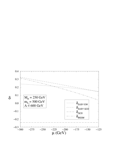
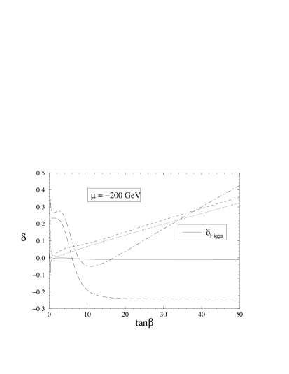
(a)	(b)
(c)	(d)

Figure 4: The $\widetilde{\mathrm{EW}}$, $\widetilde{\mathrm{QCD}}$, standard QCD and full MSSM contributions to $\delta$, eq.(15), as a function of $\mu$; (b) As in (a), but as a function of $\tan\beta$. Also shown in (b) is the Higgs contribution, $\delta_{Higgs}$; (c) As in (a), but as a function of $m_{\tilde{b}_{1}}$; (d) As a function of $m_{\tilde{t}_{1}}$. Remaining inputs as in Fig.3.

Figs.4c-4d we render the various corrections as a function of the relevant squark masses. For $m_{\tilde{b}_{1}}\stackrel{{\scriptstyle\scriptstyle<}}{{{}_{\sim}}}200\,GeV$ we observe (Cf. Fig.4c) that the $\widetilde{\mathrm{EW}}$ contribution is non-negligible ($\delta_{SUSY-EW}\simeq+20\%$) but the $\widetilde{\mathrm{QCD}}$ loops induced by squarks and gluinos are by far the leading SUSY effects ($\delta_{SUSY-QCD}>50\%$) – the standard QCD correction staying invariable over $-20\%$ and the standard EW correction (not shown) being negligible. In contrast, for larger and larger $m_{\tilde{b}_{1}}>300\,GeV$, say $m_{\tilde{b}_{1}}=400$ or $500\,GeV$, and fixed stop mass at a moderate value $m_{\tilde{t}_{1}}=150\,GeV$, the $\widetilde{\mathrm{EW}}$ output is longly sustained whereas the $\widetilde{\mathrm{QCD}}$ one steadily goes down. However, the total SUSY pay-off adds up to about $+40\%$ and the net MSSM yield still reaches a level around $+20\%$, i.e. of equal value but opposite in sign to the conventional QCD result. This would certainly entail a qualitatively distinct quantum signature.

We stress that the main parameter to decouple the $\widetilde{\mathrm{QCD}}$ correction is the lightest sbottom mass, rather than the the gluino mass [5], with which the decoupling is very slow. For this reason, since we wished to probe the regions of parameter space where these electroweak effects are important, the direct SUSY decay $H^{+}\rightarrow\tilde{t}_{i}\,\bar{\tilde{b}}_{j}$ mentioned above is blocked up kinematically and plays no role in our analysis. On the other hand, the $\widetilde{\mathrm{EW}}$ output is basically controlled by the lightest stop mass, as it is plain in Fig.4d, where we vary it in a range past the LEP$\,200$ threshold.

We have also checked that in the alternative $\mu>0$, $A_{t}<0$ scenario, the $\widetilde{\mathrm{QCD}}$ correction is negative but it is largely cancelled by the $\widetilde{\mathrm{EW}}$ part, which stays positive, so that the total $\delta_{MSSM}$ is negative and larger (in absolute value) than the standard QCD correction.

4 Conclusions

We have presented a fairly complete treatment of the supersymmetric quantum effects ($\widetilde{\mathrm{QCD}}$ and $\widetilde{\mathrm{EW}}$) on the decay width of $H^{+}\rightarrow t\,\bar{b}$ and have put forward evidence that they could be sizable enough to seriously compete with the ordinary QCD corrections. Consequently, they can either reinforce the conventional QCD corrections or counterbalance them, and even reverse their sign. This should be helpful to differentiate $H^{+}$ from alternative charged pseudoscalar decays leading to the same final states.

Our computation shows that these effects are compatible with CLEO data from low-energy $B$-meson phenomenology. We confirm that also in the constrained case the $\widetilde{\mathrm{QCD}}$ effects are generally very important (typically between $10\%-50\%$), slowly decoupling and of both signs [5]. However, we have exemplified an scenario with sparticle masses above the LEP$\,200$ discovery range where the SUSY electroweak corrections triggered by large Yukawa couplings can be comparable to the $\widetilde{\mathrm{QCD}}$ effects. In this context the total SUSY correction remains fairly large –around $+(30-50)\%$– with a $\sim 50\%$ component from electroweak supersymmetric origin. This situation occurs for

• large $\tan\beta$ ($>20$),

• huge sbottom masses ($>300\,GeV$) and

• relatively light stop and charginos ($100-200\,GeV$).

If the charged Higgs mass lies in the intermediate window (14), a chance is still left for Tevatron to produce a charged Higgs heavier than the top quark by means of “charged Higgsstrahlung” off top and bottom quarks. Should, however, a heavier $H^{\pm}$ exist outside the window (14), the LHC could continue the searching task mainly from gluon-gluon fusion where again $H^{\pm}$ is produced in association with the top quark.

The upshot is that the whole range of charged Higgs masses up to about $1\,TeV$ could be probed and, within the present renormalization framework, its potential supersymmetric nature be unravelled through a measurement of $\Gamma(H^{+}\rightarrow t\,\bar{b})$ with a modest precision of $\sim 20\%$. Alternatively, one could look for indirect SUSY quantum effects on the branching ratio of $H^{+}\rightarrow\tau^{+}\,\nu_{\tau}$ by measuring this observable to within a similar degree of precision.

Appendix

Within the context of the MSSM [1] we need two Higgs superfield doublets

$$\hat{H}_{1}=\left(\begin{array}[]{c}\hat{H}_{1}^{0}\\ \hat{H}_{1}^{-}\end{array}\right)\;\;\;\;\;,\;\;\;\;\;\hat{H}_{2}=\left(\begin{array}[]{c}\hat{H}_{2}^{+}\\ \hat{H}_{2}^{0}\end{array}\right)\,,$$ (16)

with weak hypercharges $Y_{1,2}=\mp 1$. The (neutral components of the) corresponding scalar Higgs doublets give mass to the down (up) -like quarks through the VEV $<H^{0}_{1}>=v_{1}$ ($<H^{0}_{2}>=v_{2}$). This is seen from the structure of the MSSM superpotential

$$\hat{W}=\epsilon_{ij}[h_{b}\,\hat{H}_{1}^{i}\hat{Q}^{j}\hat{D}+h_{t}\hat{H}_{2}^{j}\hat{Q}^{i}\hat{U}-\mu\hat{H}_{1}^{i}\hat{H}_{2}^{j}]\,,$$ (17)

where we have singled out only the Yukawa couplings of the third quark-squark generation, $(t,b)-(\tilde{t},\tilde{b})$, as a generic generation of chiral matter superfields $\hat{Q}$, $\hat{U}$ and $\hat{D}$. Their respective scalar (squark) components are:

$$\tilde{Q}=\left(\begin{array}[]{c}\tilde{t^{\prime}}_{L}\\ \tilde{b^{\prime}}_{L}\end{array}\right)\;\;\;,\;\;\;\tilde{U}=\tilde{t^{\prime}}_{R}^{*}\;\;\;,\;\;\;\tilde{D}=\tilde{b^{\prime}}_{R}^{*}\,,$$ (18)

with weak hypercharges $Y_{Q}=+1/3$, $Y_{U}=-4/3$ and $Y_{D}=+2/3$. The primes in (18) denote the fact that $\tilde{q^{\prime}}_{a}=\{\tilde{q^{\prime}}_{L},\tilde{q^{\prime}}_{R}\}$ are weak-eigenstates, not mass-eigenstates. The ratio

$$\tan\beta={v_{2}\over v_{1}}\,,$$ (19)

is a most relevant parameter throughout our analysis.

We briefly describe the necessary SUSY formalism:

• The fermionic partners of the weak-eigenstate gauge bosons and Higgs bosons are called gauginos, $\tilde{B}$, $\tilde{W}$, and higgsinos, $\tilde{H}$, respectively. From them we construct the mass-eigenstates, so-called charginos and neutralinos, by forming the following three sets of two-component Weyl spinors:

  $$\Gamma_{i}^{+}=\{-i\tilde{W}^{+},\tilde{H_{2}^{+}}\}\ ,\;\;\;\Gamma_{i}^{-}=\{-i\tilde{W}^{-},\tilde{H_{1}^{-}}\}\ ,$$

  $$\Gamma_{\alpha}^{0}=\{-i\tilde{B^{0}},-i\tilde{W_{3}^{0}},\tilde{H_{2}^{0}},\tilde{H_{1}^{0}}\}\ ,$$

  which get mixed up when the neutral Higgs fields acquire nonvanishing VEV’s, and diagonalizing the resulting “ino” mass Lagrangian

  $${\cal L}_{M} = -<\Gamma^{+}|\pmatrix{M&\sqrt{2}M_{W}c_{\beta}\cr\sqrt{2}M_{W}s_{\beta}&\mu}|\Gamma^{-}>$$

  $$-{1\over 2} <\Gamma^{0}| \!\!\!\!\pmatrix{M^{\prime}\!&0\!\!&M_{Z}s_{\beta}s_{W}\!&-M_{Z}c_{\beta}s_{W}\!\cr 0\!&M\!\!&-M_{Z}s_{\beta}c_{W}\!&M_{Z}c_{\beta}c_{W}\!\cr M_{Z}s_{\beta}s_{W}\!&-M_{Z}s_{\beta}c_{W}\!\!&0\!&-\mu\!\cr-M_{Z}c_{\beta}s_{W}\!&M_{Z}c_{\beta}c_{W}\!\!&-\mu\!&0\!}|\Gamma^{0}>$$

  $$+ h.c.$$ (20)

  where we remark the presence of the parameter $\mu$ introduced above and of the soft SUSY-breaking Majorana masses $M$ and $M^{\prime}$, usually related as $M^{\prime}/M=(5/3)\,\tan^{2}{\theta_{W}}$, and where $c_{\beta}=\cos\!\beta$ and $s_{\beta}=\sin\!\beta$. The corresponding mass-eigenstates are:

  $$\Psi_{i}^{+}=\pmatrix{U_{ij}\Gamma_{j}^{+}\cr V_{ij}^{*}\bar{\Gamma}_{j}^{-}}\;\;\;\;\;,\;\;\;\;\;\Psi_{i}^{-}=C\bar{\Psi_{i}}^{-T}=\pmatrix{V_{ij}\Gamma^{-}_{j}\cr U_{ij}^{*}\bar{\Gamma}_{j}^{+}}\ ,$$

  and

  $$\Psi_{\alpha}^{0}=\pmatrix{N_{\alpha\beta}\Gamma_{\beta}^{0}\cr N_{\alpha\beta}^{*}\bar{\Gamma}_{\beta}^{0}}=C\bar{\Psi}_{\alpha}^{0T}\ ,$$

  where the matrices $U,V,N$ are defined through

  $$U^{*}{\cal M}V^{\dagger}=diag\{M_{1},M_{2}\}\;,\;\;\;N^{*}{\cal M}^{0}N^{\dagger}=diag\{M_{1}^{0},\ldots,M_{4}^{0}\}\ .$$ (21)

  Among the gauginos we also have the strongly interacting gluinos, ${\tilde{g}}^{r}$ $(r=1,\ldots,8)$, which are the fermionic partners of the gluons.

• As for the scalar partners of quarks and leptons, they are called squarks, $\tilde{q}$, and sleptons, $\tilde{l}$, respectively. Again we will use the third quark-squark generation $(t,b)-(\tilde{t},\tilde{b})$ as a generic fermion-sfermion generation. The squark mass-eigenstates, $\tilde{q}_{a}=\{\tilde{q}_{1},\tilde{q}_{2}\}$, if we neglect intergenerational mixing, are obtained from the weak-eigenstate ones $\tilde{q^{\prime}}_{a}=\{\tilde{q^{\prime}}_{1}\equiv\tilde{q}_{L},\,\,\tilde{q^{\prime}}_{2}\equiv\tilde{q}_{R}\}$, through

  $$\tilde{q^{\prime}}_{a} = \sum_{b}R_{ab}^{(q)}\tilde{q}_{b},$$

  $$R^{(q)} = \pmatrix{\cos{\theta_{q}}&-\sin{\theta_{q}}\cr\sin{\theta_{q}}&\cos{\theta_{q}}}\;\;\;\;\;\;(q=t,b)\,.$$ (22)

  The rotation matrices in (22) diagonalize the corresponding stop and sbottom mass matrices:

  $${\cal M}_{\tilde{q}}^{2}=\pmatrix{M_{\tilde{q}_{L}}^{2}+m_{q}^{2}+\cos{2\beta}(T_{3}^{q_{L}}-Q_{q}s_{W}^{2})M_{Z}^{2}\ \ \ \ \ \ \ \ m_{q}M_{LR}^{q}\cr m_{q}M_{LR}^{q}\ \ \ \ \ \ \ \ M_{\tilde{q}_{R}}^{2}+m_{q}^{2}+\cos{2\beta}\,Q_{q}s_{W}^{2}M_{Z}^{2}}\,,$$ (23)

  $$R^{(q)\dagger}{\cal M}_{\tilde{q}}^{2}R^{(q)}=diag\{m_{\tilde{q}_{2}}^{2},m_{\tilde{q}_{1}}^{2}\}\ \ \ \ \ (m_{\tilde{q}_{2}}\geq m_{\tilde{q}_{1}})\,,$$ (24)

  with $T_{3}^{q_{L}}$ the third component of weak isospin, $Q$ the electric charge, and $M_{{\tilde{q}}_{L,R}}$ the soft SUSY-breaking squark masses. (By $SU(2)_{L}$-gauge invariance, we must have $M_{\tilde{t}_{L}}=M_{\tilde{b}_{L}}$, whereas $M_{{\tilde{t}}_{R}}$, $M_{{\tilde{b}}_{R}}$ are in general independent parameters.) The mixing angle on eq.(22) is given by

  $$\tan 2{\theta_{q}}={2\,m_{q}\,M_{LR}^{q}\over M_{\tilde{q}_{L}}^{2}-M_{\tilde{q}_{R}}^{2}+\cos{2\beta}(T_{3}^{q_{L}}-2Q_{q}s_{W}^{2})M_{Z}^{2}}\,,$$ (25)

  where

  $$M_{LR}^{t}=A_{t}-\mu\cot\beta\,,\ \ \ \ \ M_{LR}^{b}=A_{b}-\mu\tan\beta\,,$$ (26)

  are, respectively, the stop and sbottom off-diagonal mixing terms on eq.(23), and $A_{t,b}$ are the trilinear soft SUSY-breaking parameters.

  The charged slepton mass-eigenstates can be obtained in a similar way.

• fermion–sfermion–(chargino or neutralino)

  After translating the allowed quark-squark-higgsino/gaugino interactions into the mass-eigenstate basis, one finds

  $${\cal L}_{\Psi q\tilde{q}} = g\,\sum_{a=1,2}\sum_{i=1,2}\left(-\tilde{t}_{a}^{*}\bar{\Psi}_{i}^{-}\left(A_{+ai}^{(t)}P_{L}+A_{-ai}^{(t)}P_{R}\right)\,b\right.$$

  $$\phantom{g\,\sum_{a=1,2}\sum_{i=1,2}}-\left.\tilde{b}_{a}^{*}\bar{\Psi}_{i}^{+}\left(A_{+ai}^{(b)}P_{L}+A_{-ai}^{(b)}P_{R}\right)\,t\right)$$

  $$+ \displaystyle{\frac{g}{\sqrt{2}}} \sum_{a=1,2}\sum_{\alpha=1,\ldots,4}\left(-\tilde{t}_{a}^{*}\bar{\Psi}_{\alpha}^{0}\left(A_{+a\alpha}^{(t)}P_{L}+A_{-a\alpha}^{(t)}P_{R}\right)\,t\right.$$

  $$\phantom{\sum_{a=1,2}\sum_{\alpha=1,\ldots,4}}+\left.\tilde{b}_{a}^{*}\bar{\Psi}_{\alpha}^{0}\left(A_{+a\alpha}^{(b)}P_{L}+A_{-a\alpha}^{(b)}P_{R}\right)\,b\right)$$

  $$+$$ h.c. (27)

  where $A_{\pm ai}^{(t)},\ A_{\pm ai}^{(b)},\ A_{\pm a\alpha}^{(t)},\ A_{\pm a\alpha}^{(b)}$ are

  $$\begin{array}[]{lll}A_{+ai}^{(t)}&=&R_{1a}^{(t)*}U_{i1}^{*}-\lambda_{t}R_{2a}^{(t)*}U_{i2}^{*}\,,\\ A_{-ai}^{(t)}&=&-\lambda_{b}R_{1a}^{(t)*}V_{i2}\,,\\ A_{+a\alpha}^{(t)}&=&R_{1a}^{(t)*}\left(N_{\alpha 2}^{*}+Y_{L}\tan\theta_{W}N_{\alpha 1}^{*}\right)+\sqrt{2}\lambda_{t}R_{2a}^{(t)*}N_{\alpha 3}^{*}\,,\\ A_{-a\alpha}^{(t)}&=&\sqrt{2}\lambda_{t}R_{1a}^{(t)*}N_{\alpha 3}-Y_{R}^{t}\tan\theta_{W}R_{2a}^{(t)*}N_{\alpha 1}\,,\\ A_{+ai}^{(b)}&=&R_{1a}^{(b)*}V_{i1}^{*}-\lambda_{b}R_{2a}^{(b)*}V_{i2}^{*}\,,\\ A_{-ai}^{(b)}&=&-\lambda_{t}R_{1a}^{(b)*}U_{i2}\,,\\ A_{+a\alpha}^{(b)}&=&R_{1a}^{(b)*}\left(N_{\alpha 2}^{*}-Y_{L}\tan\theta_{W}N_{\alpha 1}^{*}\right)-\sqrt{2}\lambda_{b}R_{2a}^{(b)*}N_{\alpha 4}^{*}\,,\\ A_{-a\alpha}^{(b)}&=&-\sqrt{2}\lambda_{b}R_{1a}^{(b)*}N_{\alpha 4}+Y_{R}^{b}\tan\theta_{W}R_{2a}^{(b)*}N_{\alpha 1}\,.\end{array}$$ (28)

  with $Y_{L}$ and $Y_{R}^{t,b}$ the weak hypercharges of the left-handed $SU(2)_{L}$ doublet and right-handed singlet fermion, and $\lambda_{t}$ and $\lambda_{b}$ the potentially significant Yukawa couplings – Cf. eq.(1) – normalized to the $SU(2)_{L}$ gauge coupling constant $g$.

• quark–squark–gluino

  $${\cal L}_{{\tilde{g}}q\tilde{q}}=-\frac{g_{s}}{\sqrt{2}}\tilde{q}_{a,k}^{*}\,\bar{\tilde{g}}_{r}\left(\lambda^{r}\right)_{kl}\left(R_{1a}^{(q)*}P_{L}-R_{2a}^{(q)*}P_{R}\right)q_{l}+\mbox{ h.c.}$$ (29)

  where $\lambda^{r}$ are the Gell-Mann matrices.

• squark–squark–Higgs

  $${\cal L}_{H^{\pm}\tilde{q}\tilde{q}}=\frac{g}{\sqrt{2}M_{W}}H^{-}\tilde{b}_{a}^{*}G_{ab}\,\tilde{t}_{b}\ +\ \mbox{\rm h.c.}$$ (30)

  where we have introduced the coupling matrix

  $$G_{ab} = R_{cb}^{(t)}R_{da}^{*(b)}g_{cd}$$

  $$g_{cd} = \!\!\!\!\!\!\pmatrix{\!m_{b}^{2}\tan\beta+m_{t}^{2}\cot\!\beta-M^{2}_{W}\sin 2\beta&\!\!\!\!\!\!m_{b}\left(\mu+A_{b}\tan\beta\right)\cr m_{t}\left(\mu+A_{t}\cot\!\beta\right)&\!\!\!\!\!\!m_{t}m_{b}\left(\tan\beta+\cot\!\beta\right)\!}\,.$$ (31)

• chargino–neutralino–charged Higgs

  $${\cal L}_{H^{\pm}\Psi^{\mp}\Psi^{0}}=-g\,H^{-}\bar{\Psi}_{\alpha}^{0}\left(\cos\!\beta\;Q_{\alpha i}^{L}P_{L}+\sin\!\beta\;Q_{\alpha i}^{R}P_{R}\right)\Psi_{i}^{+}\ +\ \mbox{\rm h.c.}$$ (32)

  with

  $$\left\{\begin{array}[]{lcl}Q_{\alpha i}^{L}&=&U_{i1}^{*}N_{\alpha 3}^{*}+\frac{1}{\sqrt{2}}\left(N_{\alpha 2}^{*}+\tan\theta_{W}N_{\alpha 1}^{*}\right)U_{i2}^{*}\\ Q_{\alpha i}^{R}&=&V_{i1}N_{\alpha 4}-\frac{1}{\sqrt{2}}\left(N_{\alpha 2}+\tan\theta_{W}N_{\alpha 1}\right)V_{i2}\,.\end{array}\right.$$ (33)

References

• [1] H. P. Nilles.Phys. Rept., 110:1, 1984.
• [2] J. A. Coarasa, D. Garcia, J. Guasch, R. A. Jiménez, J. Solà. Eur. Phys. J., C2:373, 1998.
• [3] J. A. Coarasa, D. Garcia, J. Guasch, R. A. Jiménez, J. Solà. Phys. Lett., B442:326–334, 1998.
• [4] M. S. Alam et al. Phys. Rev. Lett., 74:2885–2889, 1995.
• [5] R. A. Jiménez and J. Solà. Phys. Lett., B389:53–61, 1996.