UAB-FT-451 February, 1999 hep-ph/9903212

RADIATIVE CORRECTIONS TO TOP QUARK DECAY INTO CHARGED HIGGS AT THE TEVATRON
J.A. COARASA, Jaume GUASCH, Joan SOLÀ

Grup de Física Teòrica

and

Institut de Física d’Altes Energies

Universitat Autònoma de Barcelona

08193 Bellaterra (Barcelona), Catalonia, Spain

ABSTRACT

We present the computation of the leading one-loop electroweak radiative corrections to the non-standard top quark decay width $\Gamma(t\rightarrow H^{+}\,b)$, using a physically motivated definition of $\tan\beta$. We find that the corrections are large, both in the Minimal Supersymmetric Standard Model (MSSM) and the Two-Higgs-Doublet Model (2HDM). These corrections have an important effect on the interpretation of the Tevatron data, leading to the non-existence of a model-independent bound in the $\tan\beta-M_{H^{\pm}}$ plane.

1 Introduction

The top quark has been subject of dedicated studies since its discovery at the Fermilab Tevatron Collider[1]. Due to its large mass it can develop large couplings with the Spontaneus Symmetry Breaking sector of the theory, and the Electroweak quantum corrections of this sector could be large, and indeed they are. This is specially true in some extensions of the Standard Model (SM) where this sector is enlarged, such as the Two-Higgs-Doublet Model (2HDM)[2], or the Minimal Supersymmetric Standard Model (MSSM).

Here we will present the computation of the Electroweak corrections to the non-standard top quark decay partial width into a charged Higgs particle and a bottom quark $\Gamma(t\to H^{+}\,b)$. We will present the correccions arising in generic Type I and Type II 2HDM, as well as the MSSM. We make our computation at leading order in both the Yukawa coupling of the top quark, and the Yukawa coupling of the bottom quark.

The Two-Higgs-Doublet Model ($2$HDM)[2] plays a special role as the simplest extension of the electroweak sector of the SM. After spontaneous symmetry breaking one is left with two CP-even (scalar) Higgs bosons $h^{0}$, $H^{0}$, a CP-odd (pseudoscalar) Higgs boson $A^{0}$ and a pair of charged Higgs bosons $H^{\pm}$. The parameters of these models consist of: i) the masses of the Higgs particles, $M_{h^{0}}$, $M_{H^{0}}$, $M_{A^{0}}$ and $M_{H^{+}}$ (with the convention $M_{h^{0}}<M_{H^{0}}$), ii) the ratio of the two vacuum expectation values: $\tan\beta={v_{2}/v_{1}}$, and the mixing angle $\alpha$ between the two CP-even states. Two types of such models have been of special interest[2] which avoid potentially dangerous tree-level Flavour Changing Neutral Currents: In Type I $2$HDM only one of the Higgs doublets is coupled to the fermionic sector, whereas in Type II $2$HDM each Higgs doublet ($H_{1}$, $H_{2}$) is coupled to the up-type fermions and down-type fermions respectively, the Yukawa couplings being

$$\lambda_{t}\equiv{h_{t}\over g}={m_{t}\over\sqrt{2}\,M_{W}\,\sin{\beta}}\;\;\;\;\;,\;\;\;\;\;\lambda_{b}^{\{{\rm I,\,II}\}}\equiv{h_{b}\over g}={m_{b}\over\sqrt{2}\,M_{W}\,\{\sin{\beta},\cos{\beta}\}}\,\,.$$ (1)

Type II models do appear in specific extensions of the SM, such as the Minimal Supersymmetric Standard Model (MSSM) which is currently under intensive study both theoretically and experimentally. In this latter model all the parameters of the Higgs sector are computed as a function of just two input parameters: $\tan\beta$ and a mass, which we take to be $M_{H^{+}}$ .

In case that the charged Higgs boson is light enough, the top quark could decay via the non-standard channel $t\rightarrow H^{+}\,b$. Based on this possibility the CDF collaboration at the Tevatron has undertaken an experimental program which at the moment has been used to put limits on the parameter space of Type II models[4]. The bounds are obtained by searching for an excess of the cross-section $\sigma(p\bar{p}\rightarrow t\bar{t}X\rightarrow\tau\nu_{\tau}X)$ with respect to $\sigma(p\bar{p}\rightarrow t\bar{t}X\rightarrow l\nu_{l}\,X)$ ($l=e,\,\mu$). The absence of such an excess determines an upper bound on $\Gamma(t\rightarrow H^{+}\,b\rightarrow\tau^{+}\,\nu_{\tau}\,b)$ and a corresponding excluded region of the parameter space $(\tan\beta,M_{H^{+}})$. However, it has been shown that the one-loop quantum corrections to that decay width can be rather large. This applies not only to the conventional QCD one-loop corrections[5] – the only ones used in Ref.[4] – but also to the QCD and electroweak corrections in the framework of the MSSM[6, 7, 8]. Thus the CDF limits could be substantially modified by radiative corrections[9] and in some cases the bound even disappears.

We remark that although CLEO data on $BR(b\rightarrow s\gamma)$ could preclude the existence of a light charged Higgs boson [10] – thus barring the possibility of the top quark decaying into it – this assertion is not completely general and, moreover, needs further experimental confirmation.

It is our aim to investigate, independent of and complementary to the indirect constraints, the decay $t\rightarrow H^{+}\,b$ in general $2$HDM’s (Types I and II) and in the MSSM by strictly taking into consideration the direct data from Tevatron on equal footing as in Ref.[4]. This study should be useful to distinguish the kind of quantum effects expected in general $2$HDM’s as compared to those within the context of the MSSM.

The interaction Lagrangian describing the $H\,t\,b$-vertex in Type-$j$ $2$HDM $(j=I,II)$ is:

$${\cal L}_{Htb}^{(j)}=\frac{g}{\sqrt{2}M_{W}}H^{-}\,\bar{b}\,\left[m_{t}\,\cot\beta\,P_{R}+m_{b}\,a_{j}\,P_{L}\right]\,t+{\rm h.c.}$$ (2)

where we have introduced the parameter $a_{j}$ with $a_{I}\equiv-\cot\beta$, $a_{II}\equiv+\tan\beta$. From the interaction Lagrangian (2) it is patent that for Type I models the branching ratios $BR(t\rightarrow H^{+}\,b)$ and $BR(H^{+}\rightarrow\tau^{+}\nu_{\tau})$ are relevant only at low $\tan\beta$, whereas for Type II models the former branching ratio can be important both at low and high $\tan\beta$ and the latter is only significant at high values of $\tan\beta$.

2 One-loop corrected $\Gamma(t\to H^{+}\,b)$

The renormalization procedure required for the one-loop amplitude extends that of Ref. [7]. The counterterm Lagrangian $\delta{\cal L}_{Hbt}^{(j)}$ for each $2$HDM model $j=I,II$ reads

$$\delta{\cal L}_{Hbt}^{(j)}={g\over\sqrt{2}\,M_{W}}\,H^{-}\,\bar{b}\left[\delta C_{R}^{(j)}\ m_{t}\,\cot\beta\,\,P_{R}+\delta C_{L}^{(j)}\ m_{b}\,a_{j}\,P_{L}\right]\,t+{\rm h.c.}\,,$$ (3)

with

$$\delta C_{R}^{(j)} = {\delta m_{t}\over m_{t}}-{\delta v\over v}+\frac{1}{2}\,\delta Z_{H^{+}}+\frac{1}{2}\,\delta Z_{L}^{b}+\frac{1}{2}\,\delta Z_{R}^{t}-{\delta\tan\beta\over\tan\beta}+\delta Z_{HW}\,\tan\beta\,,$$

$$\delta C_{L}^{(j)} = {\delta m_{b}\over m_{b}}-{\delta v\over v}+\frac{1}{2}\,\delta Z_{H^{+}}+\frac{1}{2}\,\delta Z_{L}^{t}+\frac{1}{2}\,\delta Z_{R}^{b}\mp{\delta\tan\beta\over\tan\beta}\,-\delta Z_{HW}\,\frac{1}{a_{j}}\,,$$ (4)

where in the last expression the upper minus sign applies to Type I models and the lower plus sign to Type II – hereafter we will adopt this convention.

The counterterm $\delta\tan\beta/\tan\beta$ is defined in such a way that it absorbs the one-loop contribution to the decay width $\Gamma(H^{+}\rightarrow\tau^{+}\nu_{\tau})$, yielding

$${\delta\tan\beta\over\tan\beta}=\mp\left[{\delta v\over v}-\frac{1}{2}\delta Z_{H^{\pm}}+\delta Z_{HW}\frac{1}{a_{j}}+\Delta_{\tau}^{(j)}\,\right]\,\,.$$ (5)

The quantity

$$\Delta_{\tau}^{(j)}=-{\delta m_{\tau}\over m_{\tau}}-\frac{1}{2}\delta Z_{L}^{\nu_{\tau}}-\frac{1}{2}\delta Z_{R}^{\tau}-F_{\tau}^{(j)}\,,$$ (6)

contains the (finite) process-dependent part of the counterterm, where $F_{\tau}$ comprises the complete set of one-particle-irreducible three-point functions of the charged Higgs decay into $\tau^{+}\,\nu_{\tau}$.

The correction to the decay width in each $2$HDM is defined as

$$\delta_{\rm 2HDM}^{(j)}=\frac{\Gamma^{(j)}(t\rightarrow H^{+}\,b)-\Gamma_{0}^{(j)}(t\rightarrow H^{+}\,b)}{\Gamma_{0}^{(j)}(t\rightarrow H^{+}\,b)}$$ (7)

where $\Gamma_{0}^{(j)}$ is the lowest-order width in the on-shell $\alpha$-scheme .

The renormalized one-loop vertices $\Lambda_{L,R}$ for each type of model are obtained after adding up the counterterms (4) to the one-loop form factors:

$$\Lambda_{L} = \delta C_{L}+F_{L}$$

$$\Lambda_{R} = \delta C_{R}+F_{R}\,\,\,.$$ (8)

The one-loop Feynman diagrams contributing to the decay $t\rightarrow H^{+}b$ under consideration can be seen in Ref. [7]. For the $2$HDM one just must take the Higgs bosons mediated diagrams: Fig. 3 (all diagrams), Fig. 4 (diagrams $C_{b3}$, $C_{b4}$, $C_{t3}$, $C_{t4}$), Fig. 5 (diagram $C_{H1}$) and Fig. 6 (diagram $C_{M1}$) of that reference. It goes without saying that the calculation of these diagrams in general $2$HDM’s is different from that in Ref.[7], and this is so even for the Type II case since some of the Higgs boson Feynman rules for supersymmetric models[2] cannot be borrowed without a careful adaptation of the couplings .

2.1 Vertex functions

Now we consider contributions arising from the exchange of virtual Higgs particles and Goldstone bosons in the Feynman gauge, as shown in Fig.3 of Ref. [7]. We follow the vertex formula for the form factors by the value of the overall coefficient $N$ and by the arguments of the corresponding $3$-point functions.

We start by defining the following factors for each Type-$j$ 2HDM:

$$R_{j} = \{\sin\alpha/\sin\beta,\cos\alpha/\cos\beta\}\,\,,$$

$$r_{j} = \{\cos\alpha/\sin\beta,-\sin\alpha/\cos\beta\}\,\,,$$

then the contributions from the different diagrams can be written as

• Diagram $(V_{H1})$:

  $$F_{L} = N\,[m_{b}^{2}(C_{12}-C_{0})+m_{t}^{2}\frac{\cot\!\beta}{a_{j}}(C_{11}-C_{12})]\,,$$

  $$F_{R} = Nm_{b}^{2}[C_{12}-C_{0}+\frac{a_{j}}{\cot\!\beta}(C_{11}-C_{12})]\,,$$

  $$N = -\frac{ig^{2}}{2}\{R_{j},r_{j}\}N_{1}\,,$$

  $$N_{1} = \frac{M^{2}_{A^{0}}-M_{\{H^{0},h^{0}\}}^{2}}{M^{2}_{W}}\cot\!2\beta\{\sin\!(\alpha-\beta),\cos\!(\alpha-\beta)\}+$$ (9)

  $$\frac{M^{2}_{A^{0}}-M_{H^{\pm}}^{2}-M_{\{H^{0},h^{0}\}}^{2}/2}{M^{2}_{W}}\{\cos(\beta-\alpha),\sin(\beta-\alpha)\}\,,$$

  where $C_{*}$ are the usual one-loop scalar three-point functions [14]. In eq. (9) they must be evaluated with arguments

  $$C_{*}=C_{*}\left(p,p^{\prime},m_{b},M_{H^{\pm}},\{M_{H^{0}},M_{h^{0}}\}\right)\,.$$

• Diagram $(V_{H2})$:

  $$F_{L} = N\frac{1}{a_{j}}[m_{t}^{2}(C_{11}-C_{12})+m_{b}^{2}(C_{0}-C_{12})]\,,$$

  $$F_{R} = Nm_{b}^{2}\tan\beta(2C_{12}-C_{11}-C_{0})\,,$$

  $$N = \pm\frac{ig^{2}}{4}\{R_{j},r_{j}\}\{\sin(\beta-\alpha),\cos(\beta-\alpha)\}\left(\frac{M^{2}_{H^{\pm}}}{M^{2}_{W}}-\frac{\{M^{2}_{H^{0}},M_{h^{0}}^{2}\}}{M^{2}_{W}}\right)\,,$$

  $$C_{*} = C_{*}\left(p,p^{\prime},m_{b},M_{W},\{M_{H^{0}},M_{h^{0}}\}\right)\,.$$

• Diagram $(V_{H3})$:

  $$F_{L} = Nm_{t}^{2}[\frac{\cot\!\beta}{a_{j}}C_{12}+C_{11}-C_{12}-C_{0}]\,,$$

  $$F_{R} = N\,[m_{b}^{2}\frac{a_{j}}{\cot\!\beta}C_{12}+m_{t}^{2}(C_{11}-C_{12}-C_{0})]\,,$$

  $$N = -\frac{ig^{2}}{2}\frac{\{\sin\alpha,\cos\alpha\}}{\sin\beta}N_{1}\,,$$

  $$C_{*} = C_{*}\left(p,p^{\prime},m_{t},\{M_{H^{0}},M_{h^{0}}\},M_{H^{\pm}}\right)\,.$$

• Diagram $(V_{H4})$:

  $$F_{L} = Nm_{t}^{2}(2C_{12}-C_{11}+C_{0})\frac{1}{a_{j}}\,,$$

  $$F_{R} = N\,[-m_{b}^{2}C_{12}+m_{t}^{2}(C_{11}-C_{12}-C_{0})]\tan\beta\,,$$

  $$N = \mp\frac{ig^{2}}{4}\frac{\{\sin\alpha\sin(\beta-\alpha),\cos\alpha\cos(\beta-\alpha)\}}{\sin\beta}\left(\frac{M^{2}_{H^{\pm}}}{M^{2}_{W}}-\frac{\{M^{2}_{H^{0}},M_{h^{0}}^{2}\}}{M^{2}_{W}}\right)\,,$$

  $$C_{*} = C_{*}\left(p,p^{\prime},m_{t},\{M_{H^{0}},M_{h^{0}}\},M_{W}\right)\,.$$

• Diagram $(V_{H5})$:

  $$F_{L} = N\,[m_{b}^{2}(C_{12}+C_{0})+m_{t}^{2}(C_{11}-C_{12})]\,,$$

  $$F_{R} = Nm_{b}^{2}\frac{a_{j}}{\cot\!\beta}(C_{11}+C_{0})\,,$$

  $$N = -\frac{ig^{2}}{4}\left(\frac{M^{2}_{H^{\pm}}}{M^{2}_{W}}-\frac{M^{2}_{A^{0}}}{M^{2}_{W}}\right)\,,$$

  $$C_{*} = C_{*}\left(p,p^{\prime},m_{b},M_{W},M_{A^{0}}\right)\,.$$

• Diagram $(V_{H6})$:

  $$F_{L} = Nm_{t}^{2}\frac{\cot\!\beta}{a_{j}}(C_{11}+C_{0})\,,$$

  $$F_{R} = N\,[m_{b}^{2}C_{12}+m_{t}^{2}(C_{11}-C_{12}+C_{0})]\,,$$

  $$N = -\frac{ig^{2}}{4}\left(\frac{M^{2}_{H^{\pm}}}{M^{2}_{W}}-\frac{M^{2}_{A^{0}}}{M^{2}_{W}}\right)\,,$$

  $$C_{*} = C_{*}\left(p,p^{\prime},m_{t},M_{A^{0}},M_{W}\right)\,.$$

• Diagram $(V_{H7})$:

  $$F_{L} = N\,[(2m_{b}^{2}C_{11}+\tilde{C}_{0}+2(m_{t}^{2}-m_{b}^{2})(C_{11}-C_{12}))\frac{\cot\!\beta}{a_{j}}$$

  $$+2m_{b}^{2}(C_{11}+2C_{0})]m_{t}^{2}\,,$$

  $$F_{R} = N\,[(2m_{b}^{2}C_{11}+\tilde{C}_{0}+2(m_{t}^{2}-m_{b}^{2})(C_{11}-C_{12}))\frac{a_{j}}{\cot\!\beta}$$

  $$+2m_{t}^{2}(C_{11}+2C_{0})]m_{b}^{2}\,,$$

  $$N = \frac{ig^{2}}{4M^{2}_{W}}\left\{\frac{\sin\alpha}{\sin\beta}R_{j}\,,\frac{\cos\alpha}{\sin\beta}r_{j}\right\}\,,$$

  $$C_{*} = C_{*}\left(p,p^{\prime},\{M_{H^{0}},M_{h^{0}}\},m_{t},m_{b}\right)\,.$$

• Diagram $(V_{H8})$:

  $$F_{L} = Nm_{t}^{2}\{\frac{\cot\!\beta}{a_{j}}\,,\cot^{2}\!\beta\}\,\tilde{C}_{0}\,,$$

  $$F_{R} = Nm_{b}^{2}\{\frac{a_{j}}{\cot\!\beta}\,,\tan^{2}\!\beta\}\,\tilde{C}_{0}\,,$$

  $$N = \mp\frac{ig^{2}}{4M^{2}_{W}}\,,$$

  $$C_{*} = C_{*}\left(p,p^{\prime},\{M_{A^{0}},M_{Z}\},m_{t},m_{b}\right)\,.$$

2.2 Counterterms

The diagrammatic contributions to the various counterterms in eq. (4) can bee seen in Ref. [7]: in Fig. 4 (diagrams $C_{b3}$, $C_{b4}$, $C_{t3}$, $C_{t4}$) the external fermion counterterms; In Fig. 5 (diagram $C_{H1}$) the charged Higgs particle counterterms; And in Fig. 6 (diagram $C_{M1}$) the contribution to the $W^{\pm}-H^{\pm}$ mixing self-energy contributions. Now we pass to the explicit expression of that counterterms.

• Counterterms $\delta m_{f}\,,\delta Z_{L}^{f}\,,\delta Z_{R}^{f}$: For a given down-like fermion $b$, and corresponding isospin partner $t$, the fermionic self-energies receive contributions

  $$\Sigma_{\{L,R\}}^{b}(p^{2}) = \left.\Sigma_{\{L,R\}}^{b}(p^{2})\right|_{(C_{b3})+(C_{b4})}=\frac{g^{2}}{2iM^{2}_{W}}$$

  $$\times \left\{m_{\{t,b\}}^{2}\left[\{\cot^{2}\!\beta,a_{j}^{2}\}B_{1}(p,m_{t},M_{H^{\pm}})+B_{1}(p,m_{t},M_{W})\right]\right.$$

  $$+ \frac{m_{b}^{2}}{2}\left[R_{j}^{2}\,B_{1}(p,m_{b},M_{H^{0}})+r_{j}^{2}\,B_{1}(p,m_{b},M_{h^{0}})\right.$$

  $$\ \ \ +\left.\left.a_{j}^{2}\,B_{1}(p,m_{b},M_{A^{0}})+B_{1}(p,m_{b},M_{Z})\right]\right\}\,,$$

  $$\Sigma_{S}^{b}(p^{2}) = \left.\Sigma_{S}^{b}(p^{2})\right|_{(C_{b3})+(C_{b4})}$$ (10)

  $$= -\frac{g^{2}}{2iM^{2}_{W}}\left\{m_{t}^{2}a_{j}\cot\beta\left[B_{0}(p,m_{t},M_{H^{\pm}})-B_{0}(p,m_{t},M_{W})\right]\right.$$

  $$+ \frac{m_{b}^{2}}{2}\left[R_{j}^{2}\,B_{0}(p,m_{b},M_{H^{0}})+r_{j}^{2}\,B_{0}(p,m_{b},M_{h^{0}})\right.$$

  $$\ \ \ -\left.\left.a_{j}^{2}\,B_{0}(p,m_{b},M_{A^{0}})-\,B_{0}(p,m_{b},M_{Z})\right]\right\}\,,$$

  from Higgs and Goldstone bosons in the Feynman gauge. To obtain the corresponding expressions for an up-like fermion, $t$, just perform the label substitutions $b\leftrightarrow t$ and replace $R_{j}\to\sin\alpha/\sin\beta$, $r_{j}\to\cos\alpha/\sin\beta$, $a_{j}\leftrightarrow\cot\beta$ on eq. (• ‣ 2.2).

  Now one must introduce that expressions into the standard on-shell definitions of $\delta m_{f}$ and $\delta Z_{L,R}^{f}$ (see e.g. eqs.(20) and (21) of Ref. [7]).

• Counterterm $\delta Z_{H^{\pm}}$:

  $$\delta Z_{H^{\pm}} = \left.\delta Z_{H^{\pm}}\right|_{(C_{H1})}=\,\Sigma_{H^{\pm}}^{\prime}(M^{2}_{H^{\pm}})$$ (11)

  $$= -\frac{ig^{2}N_{C}}{M^{2}_{W}}\left[(m_{b}^{2}a_{j}^{2}+m_{t}^{2}\cot^{2}\!\beta)(B_{1}+M^{2}_{H^{\pm}}B_{1}^{\prime}+m_{b}^{2}B_{0}^{\prime})\right.$$

  $$\left.\mbox{\hskip 42.67912pt}+2\cot\beta a_{j}m_{b}^{2}m_{t}^{2}B_{0}^{\prime}\right](M_{H^{\pm}},m_{b},m_{t})\,.$$

• Counterterm $\delta Z_{HW}$:

  $$\delta Z_{HW} = \left.\delta Z_{HW}\right|_{(C_{M1})}=\frac{\Sigma_{HW}(M^{2}_{H^{\pm}})}{M^{2}_{W}}$$

  $$= - \frac{ig^{2}N_{C}}{M^{2}_{W}}\left[m_{b}^{2}a_{j}(B_{0}+B_{1})+m_{t}^{2}\cot\beta B_{1}\right](M_{H^{\pm}},m_{b},m_{t})\,.$$ (12)

  A sum is understood over all generations.

3 Numerical analysis

In the numerical analysis presented in Figs. 1-6 we have put several cuts on our set of inputs[11]. For $\tan\beta$ we have restricted in principle to the segment

$$0.1\stackrel{{\scriptstyle\scriptstyle<}}{{{}_{\sim}}}\tan\beta\stackrel{{\scriptstyle\scriptstyle<}}{{{}_{\sim}}}60\,\,\,.$$ (13)

For the three Higgs bosons coupling we have imposed that they do not exceed the maximum unitarity level permitted for the SM three Higgs boson coupling, i.e.

$$|\lambda_{HHH}|\stackrel{{\scriptstyle\scriptstyle<}}{{{}_{\sim}}}|\lambda_{HHH}^{SM}(m_{H}=1\,TeV)|=g\frac{3}{2}\frac{(1\,TeV)^{2}}{M_{W}}\,\,.$$ (14)

This condition restricts both the ranges of masses and of $\tan\beta$. Moreover, we have imposed that the extra induced contributions to the $\rho$ parameter are bounded by the current experimental limit  :

$$|\Delta\rho|\leq 0.003\,\,.$$ (15)

Of course in the MSSM analysis we apply all current limits on the SUSY particles masses and parameters.

Before exploring the implications for the Tevatron analyses, we wish to show the great sensitivity (through quantum effects) of the decay $t\rightarrow H^{+}\,b$ to the particular structure of the underlying $2$HDM. In all cases we present our results in a significant region of the parameter space where the branching ratios $BR(t\rightarrow H^{+}\,b)$ and $BR(H^{+}\rightarrow\tau^{+}\,\nu_{\tau})$ are expected to be sizeable. This entails relatively light charged Higgs bosons ($M_{H^{+}}\stackrel{{\scriptstyle\scriptstyle<}}{{{}_{\sim}}}150\,GeV$) and a low (high) value of $\tan\beta$ for Type I (II) models.

Figure 1: The correction $\delta$, eq. (7), to the decay width $\Gamma(t\rightarrow H^{+}b)$ as a function of $\tan\beta$, for Type I $2$HDM’s (left hand side of the figure) and two sets of inputs $\{(M_{H^{+}},M_{H^{0}},M_{h^{0}},M_{A^{0}});\,\tan\alpha\}$, namely set A: $\{(70,175,100,50)\,GeV;\,3\}$ and set B: $\{(120,200,80,250)\,GeV;1\}$. Similarly for Type II models (right hand side of the figure) and for two different sets of inputs, set A: $\{(120,300,50,225)\,GeV;\,1\}$ and set B: $\{(120,300,80,225)\,GeV;\,-3\}$. Shown are the electroweak contribution $\delta_{\rm EW}$ and the total correction $\delta_{\rm Total}=\delta_{\rm EW}+\delta_{\rm QCD}$.

In Fig. 1 we display the evolution of the correction (7) with $\tan\beta$ for Types I and II $2$HDM’s and for two sets of inputs A and B for each model. We separately show the (leading) EW contribution, $\delta_{\rm EW}$, and the total correction, $\delta_{\rm Total}\equiv\delta_{\rm EW}+\delta_{\rm QCD}$, which incorporates the conventional QCD effects[5]. In the relevant $\tan\beta$ segments, that is below and above the uninteresting one, we find that the pure EW contributions can be rather large, to wit: For Type I models, the positive effects can reach $\simeq 30\%$, while the negative contributions may increase ‘arbitrarily’ – thus effectively enhancing to a great extent the modest QCD corrections– still in a region of parameter space respecting the various imposed restrictions; For Type II models, instead, the EW effects can be very large, for both signs, in the high $\tan\beta$ regime. In particular, the huge positive yields could go into a complete “screening” of the QCD corrections.

(a)	(b)

Figure 2: The correction $\delta$, eq. (7), $\Gamma(t\rightarrow H^{+}b)$ as a function of $\tan\beta$, for the MSSM and for two different scenarios, (a) set A: {$M_{H^{\pm}}$=120, $\mu=-90$, M=150, $m_{\tilde{b}_{1}}$=150, $m_{\tilde{t}_{1}}$=100, $m_{\tilde{u}}=m_{\tilde{\nu}}$=400, $m_{\tilde{g}}$=300, $A_{t}=A_{b}=A_{up}=A_{l}$=300} GeV (b) set B: {$M_{H^{\pm}}$=120, $\mu=+90$, M=150 , $m_{\tilde{b}_{1}}$=$m_{\tilde{t}_{1}}$=400, $m_{\tilde{u}}=m_{\tilde{\nu}}$=400, $m_{\tilde{g}}$=1000, $A_{t}=-500$, $A_{b}=A_{up}=A_{l}$=300 } GeV. Shown are: the Higgs sector contribution $\delta_{\rm Higgs}$; the contribution from the supersymmetric electroweak sector $\delta{\rm SUSY-EW}$; the supersymmetric QCD contribution $\delta_{QCD}$; the standard QCD contribution $\delta_{QCD}$; and the total correction $\delta_{\rm Total}$.

In Fig. 2 we present the partial and total corrections in the case of the MSSM. We present separately: the standard QCD corrections; the supersymmetric (gluino-mediated) QCD correction[6]; the Higgs boson contributions; the supersymmetric contributions from the electroweak sector[7]; and the total correction, namely the net sum of all of the above contributions. In Fig. 2a we present and scenario with $\mu<0$, and a relatively light sparticle spectrum. In Fig. 2b an scenario with $\mu>0$ and a heavy mass spectrum is presented. The leading contribution to the MSSM correction is the bottom quark mass finite threshold corrections –see eq.(4)– which reads[7]

$$\left({\delta m_{b}\over m_{b}}\right)_{\scriptscriptstyle{\rm SUSY-QCD}} = -{2\alpha_{s}(m_{t})\over 3\pi}\,m_{\tilde{g}}{\mu\,}{\tan\beta}\,I(m_{\tilde{b}_{1}},m_{\tilde{b}_{2}},m_{\tilde{g}})\,,$$

$$\left({\delta m_{b}\over m_{b}}\right)_{\scriptscriptstyle{\rm SUSY-Yukawa}} = -{h_{t}^{2}\over 16\pi^{2}}\,{\mu\,A_{t}}{\tan\beta}\,I(m_{\tilde{t}_{1}},m_{\tilde{t}_{2}},\mu)\,,$$ (16)

where $I(m_{1},m_{2},m_{3})$ (given in Ref.[7]) is a slowly varying positive-definite function. We must emphasize that the presence of such a leading term (and its expression) depends on the renormalization scheme, that is, on the definition of $\tan\beta$ (5). In Fig. 2a ($\mu<0$ scenario) the positive SUSY-QCD contribution compensates the large negative QCD corrections, and thus the effect of the SUSY-EW sector are clearly visible. There is a region (around $\tan\beta\simeq 50$) where the SUSY-QCD correction fully cancels the QCD one, and we are left with only the SUSY-EW correction. The $\mu>0$ scenario (Fig. 2b) is very different. The large negative SUSY-QCD corrections add up to the already large QCD ones, the positive (due to the $\mu\,A_{t}<0$ constraint) EW corrections can not be large enough to compensate for them.

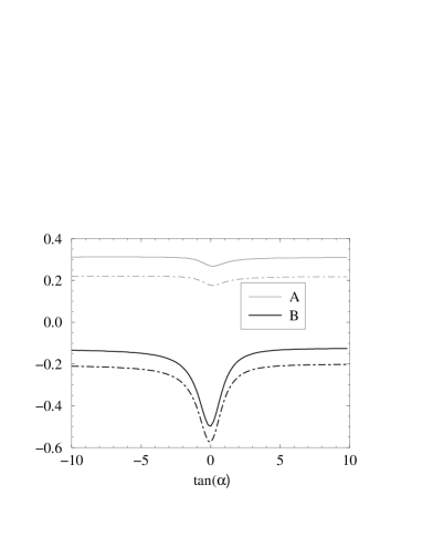
(a)	(b)
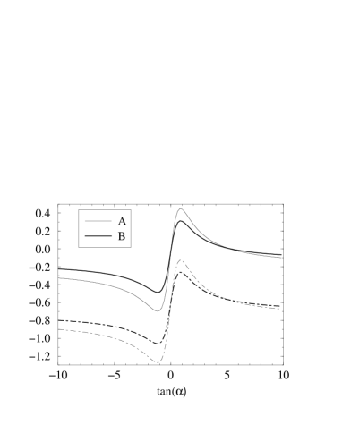
(c)	(d)

Figure 3: The corrections $\delta_{\rm EW}$ and $\delta_{\rm Total}$ (a) for the Type I $2$HDM as a function of $\tan\alpha$, inputs as in Fig. 1 with $\tan\beta=0.1$ for set A and $\tan\beta=0.2$ for set B, (b) as in (a) but for the pseudoscalar Higgs mass, (c) as in (a) but for Type II $2$HDM with $\tan\beta=35$ for both sets, (d) as in (c) but for the pseudoscalar Higgs mass.

Note that the Higgs contribution $\delta_{\rm Higgs}$ in Fig. 2 is much smaller than the other ones. After imposing the SUSY couplings in the vertex formulae of Sect. 2 there is a large cancellation among the various contributions. The reason can be seen in Fig. 3 where we present the evolution of the corrections with $\tan\alpha$ and the pseudoscalar Higgs boson mass. We see that the large corrections are attained for a specific scenario: a definite value of $\tan\alpha$ (Figs. 3a and c) and large mass splitting (Figs. 3b and d). These conditions cannot be fulfilled in the MSSM, as $\tan\alpha$ and the mass splitting are functions of the input parameters $\tan\beta$ and $M_{H^{+}}$. The evolution of the corrections with $\tan\alpha$ of the Type I $2$HDM (Fig. 3a) illustrates the general behaviour of the low $\tan\beta$ regime for both types of $2$HDM.

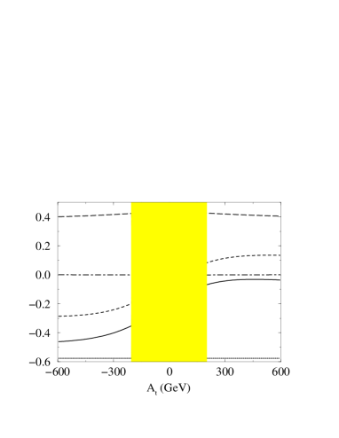
Figure 4: The correction $\delta$ for the MSSM as a function of the Soft-SUSY-breaking trilinear coupling $A_{t}$. Inputs as in as in Fig. 2(a). Shown are the same contributions as in Fig. 2.

In Fig. 4 we present the evolution with the Soft-SUSY-Breaking trilinear coupling of top squarks, which governs the behavior of the SUSY-EW corrections (16). We can see that they effectively change sign with $A_{t}$, though the full correction deviates a bit of the leading linear behaviour of eq. (16). The shaded region around $A_{t}\simeq 0$ is excluded by the conditions on the squark masses.

4 Implications for the Tevatron data

Next we turn to the discussion of the dramatic implications that the EW effects may have for the decay $t\rightarrow H^{+}\,b$ at the Tevatron. The original analysis of the data (based on the non-observation of any excess of $\tau$-events) and its interpretation in terms of limits on the $2$HDM parameter space was performed in Ref.[4] (for Type II models) without including the EW corrections. In these references an exclusion plot is presented in the $(\tan\beta,M_{H^{+}})$-plane after correcting for QCD effects only. The production cross-section of the top quark in the ($\tau$,$l$)-channel can be easily related to the decay rate of $t\rightarrow H^{+}\,b$ and the branching ratio of $H^{+}\rightarrow\tau^{+}\,\nu_{\tau}$ as follows:

$$\sigma_{l\tau}=\left[\frac{4}{81}\,\epsilon_{1}+\frac{4}{9}\,{\Gamma(t\rightarrow H^{+}\,b)\over\Gamma(t\rightarrow W^{+}\,b)}\,BR(H^{+}\rightarrow\tau^{+}\,\nu_{\tau})\,\epsilon_{2}\right]\,\sigma_{t\bar{t}}\,,$$ (17)

with

$$BR(H^{+}\rightarrow\tau^{+}\,\nu_{\tau})=\frac{\Gamma(H^{+}\rightarrow\tau^{+}\,\nu_{\tau})}{\Gamma(H^{+}\rightarrow\tau^{+}\,\nu_{\tau})+\Gamma(H^{+}\rightarrow c\,\bar{s})}\,\,,$$ (18)

where we use the QCD-corrected amplitude for the last term in the denominator[15].

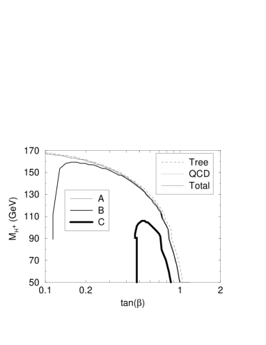
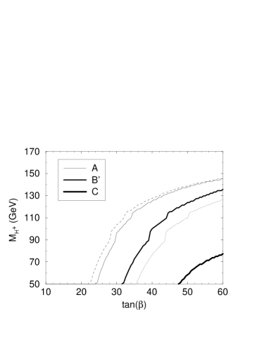
(a)	(b)

Figure 5: The $95\%$ C.L. exclusion plot in the $(\tan\beta,M_{H^{+}})$-plane for (a) Type I $2$HDM using three sets of inputs: A and B as in Fig. 1, and C: $\{(M_{H^{+}},200,80,700)\,GeV;\,1\}$; (b) Similarly for Type II models including three sets of inputs: A as defined in Fig. 1, B’:$\{(M_{H^{+}},200,80,150)\,GeV;\,0.3\}$, and C:$\{(M_{H^{+}},200,80,150)\,GeV;\,-3\}$. Shown are the tree-level, QCD-corrected and fully 2HDM-corrected contour lines. The excluded region in each case is the one lying below these curves

From Figs. 5 and 6 we inmediately see the impact of the loop effects both in the general $2$HDM and the MSSM. We have plotted the perturbative exclusion regions in the parameter space $(\tan\beta,M_{H^{+}})$ for intermediate and extreme sets of $2$HDM inputs A, B, B’ and C (Figs. 5a and b) and for the MSSM sets A and B (Fig. 6). In Type I models (5a) we see that the bounds obtained from the EW-corrected amplitude are generally less restrictive than those obtained by means of tree-level and QCD-corrected amplitudes. Evolution of the excluded region from set A to set C in Fig. 5a shows that the region tends to evanesce, which is indeed the case when we further increase $M_{A^{0}}$ in set C. In Type II models (5b) we also show a series of possible scenarios. We have checked that the maximum positive effect $\delta_{EW}>0$ (set A in Fig.5b) may completely cancel the QCD corrections and restore the full one-loop width $\Gamma^{(II)}(t\rightarrow H^{+}\,b)$ to the tree-level value just as if there were no QCD corrections at all! Intermediate possibilities (set B’) are also shown. In the other extreme the (negative) effects $\delta_{EW}<0$ enforce the exclusion region to draw back to curve C where it starts to gradually disappear into a non-perturbative corner of the parameter space where one cannot claim any bound whatsoever!!.

Figure 6: The $95\%$ C.L. exclusion plot in the $(\tan\beta,M_{H^{+}})$-plane for the MSSM. Shown are the excluded region using: the tree-level prediction for $\Gamma(t\to H^{+}\,b)$; the standard QCD prediction; and the full MSSM predictions for sets A and B as in Fig. 2.

In the MSSM we find a similar behaviour. For the first scenario ($\mu<0$) the large positive SUSY corrections take the exclusion region up to the tree-level expectation. In the scenario characterized by $\mu>0$ the large negative corrections take this region to too low values of $M_{H^{+}}$ and too high values of $\tan\beta$ and one cannot claim any bound on the $\tan\beta-M_{H^{+}}$ plane.

5 Conclusions

In the MSSM case, the Higgs sector is of Type II. However, due to supersymmetric restrictions in the structure of the Higgs potential, there are large cancellations between the one-particle-irreducible vertex functions, so that the overall contribution from the MSSM Higgs sector to the correction (7) is negligible. In fact, we have checked that when we take the Higgs boson masses as they are correlated by the MSSM we obtain the same result. Still, in the SUSY case there emerges a large effect from the genuine sparticle sector, mainly from the SUSY-QCD contributions to the bottom mass renormalization counterterm[7], which can be positive or negative because the correction flips sign with the higgsino mixing parameter (16). In contrast, for general (non-SUSY) Type II models the bulk of the EW correction comes from large unbalanced contributions from the vertex functions, which can also flip sign with $\tan\alpha$ (Cf. Fig. 3c) – a free parameter in the non-supersymmetric case. Although the size and sign of the effects can be similar for a general Type II and a SUSY $2$HDM, they should be distinguishable since the large corrections are attained for very different values of the Higgs boson masses[11].

We have demonstrated that in both cases (SUSY and general $2$HDM) the loop effecs may completely distort the previous analyses presented by the Tevatron collaborations.

References

[1]
F. Abe et al. (CDF Collab.),
Phys. Rev. Lett.74
(1995) 2626;
S. Abachi et al. (D Collab.),
Phys. Rev. Lett.74
(1995) 2632.
[2]
J.F. Gunion, H.E. Haber, G.L. Kane, S. Dawson,
The Higgs Hunters’
Guide (Addison-Wesley, Menlo-Park, 1990).
[3] A. Dabelstein, Z. Phys.C67 (1995) 495.
[4]
B. Bevensee, proceedings of the
Int. Workshop on Quantum Effects
in the MSSM, Barcelona, September 9-13 (1997),
World Scientific 1998,
Ed. J. Solà;
F. Abe et al. (CDF Collab.),
Phys. Rev. Lett.79
(1997) 357; ibid.Phys. Rev.D54 (1996) 735.
[5]
A. Czarnecki, S. Davidson, Phys. Rev.D48 (1993) 4183; ibid.D47 (1993) 3063, and references therein.
[6]
J. Guasch, R.A. Jiménez, J. Solà,
Phys. Lett.B360
(1995) 47.
[7]
J. A. Coarasa, D. Garcia, J. Guasch,
R.A. Jiménez, J. Solà,
Eur. Phys. J.C2 (1998) 373.
[8]
J. Guasch, Ph. D. Thesis, Universitat
Autònoma de Barcelona, 1999.
[9]
J. Guasch, J. Solà, Phys. Lett. B416 (1998) 353.
[10]
M.S. Alam et al. (CLEO Collab.), Phys. Rev. Lett.74 (1995) 2885.
[11]
J. A. Coarasa, J. Guasch, W. Hollik, J. Solà,
Phys. Lett.B442 (1998) 326.
[12]
W. Hollik, Z. Phys.C32
(1986) 291; C37 (1988) 569.
[13]
J. A. Coarasa, Ph. D. Thesis, Universitat
Autònoma de Barcelona, 1999.
[14]
G. ‘t Hooft, M. Veltman, Nucl. Phys.B 153 (1979) 365;
G. Passarino, M. Veltman, Nucl.Phys.B 160 (1979) 151;
A. Axelrod, Nucl. Phys.B 209 (1982) 349.