CERN-TH/99-40
hep-ph/9903203   Aspects of Neutrino Masses and Lepton-Number Violation
in the light of the Super-Kamiokande data  

Abstract

Abstract: We discuss aspects of neutrino masses and lepton-number violation, in the light of the observations of Super-Kamiokande. As a first step, we use the data from various experiments, in order to obtain a phenomenological understanding of neutrino mass textures. We then investigate how the required patterns of neutrino masses and mixings are related to the flavour structure of the underlying theory. In supersymmetric extensions of the Standard Model, renormalisation group effects can have important implications: for small $\tan\beta$, $b$–$\tau$ unification indicates the presence of significant $\mu$–$\tau$ flavour mixing. The evolution of the neutrino mixing may be described by simple semi-analytic expressions, which confirm that, for large $\tan\beta$, very small mixing at the GUT scale may be amplified to maximal mixing at low energies, and vice versa. Passing to specific models, we first discuss the predictions for neutrino masses in different GUT models (including superstring-embedded solutions). Imposing the requirement for successful leptogenesis may give additional constraints on the generic structure of the neutrino mass textures. Finally, we discuss direct ways to look for lepton-number violation in ultra-high energy neutrino interactions.

.

]

I Neutrino data and Implications

Recent reports by Super-Kamiokande [1] and other experiments [2], support previous measurements of a $\nu_{\mu}/\nu_{e}$ ratio in the atmosphere that is significantly smaller than the theoretical expectations. The data favours $\nu_{\mu}$–$\nu_{\tau}$ oscillations, with

$$\delta m_{\nu_{\mu}\nu_{\tau}}^{2} \approx (10^{-2}\;{\rm to}\;10^{-3})\;{\rm eV^{2}}$$ (1)

$$\sin^{2}2\theta_{\mu\tau} \geq 0.8$$ (2)

(Oscillations involving a sterile neutrino are also plausible, while dominant $\nu_{\mu}\rightarrow\nu_{e}$ oscillations are disfavoured by Super-Kamiokande [1] and CHOOZ  [3].).

On the other hand, the solar neutrino puzzle can be resolved through either vacuum or matter-enhanced (MSW) oscillations. The first require a mass splitting of the neutrinos that are involved in the oscillations in the range $\delta m_{\nu_{e}\nu_{\alpha}}^{2}\approx(0.5-1.1)\times 10^{-10}~{}{\rm eV}^{2}$, where $\alpha$ is $\mu$ or $\tau$. MSW oscillations on the other hand [4], allow for both small and large mixing, while now $\delta m_{\nu_{e}\nu_{\alpha}}^{2}\approx(0.3-20)\times 10^{-5}~{}{\rm eV}^{2}$. Moreover, the LSND collaboration has reported evidence for the appearance of $\overline{\nu}_{\mu}$–$\overline{\nu}_{e}$ and ${\nu}_{\mu}$–${\nu}_{e}$ oscillations [5], which however are not supported by KARMEN 2 [6]. Finally, if neutrinos were to provide a hot dark matter component, then the heavier neutrino(s) should have mass in the range $\sim(1-6)$ eV.

The implications of these observations are very interesting, since they point towards a non-zero neutrino mass and lepton-number violation, that is the existence of physics beyond the standard model. The simplest class of solutions that one may envisage consist of an extension of the Standard Model to include three new right-handed neutrino states, with a mass structure directly related to that of the other fermions. Three neutrino masses allow only two independent mass differences and thus the direct indications for neutrino oscillations discussed above cannot be simultaneously explained unless a sterile light-neutrino state is introduced. Since the LSND results have not been confirmed, in our analysis we chose not to introduce sterile states (which inevitably break any simple connection of the neutrino masses with the known charge lepton and quark hierarchies). Instead, we focus on the Super-Kamiokande and the solar neutrino data, and leave open the possibility of neutrinos as hot dark matter.

In this framework, both the solar and atmospheric deficits require small mass differences, and thus can be explained by two possible neutrino hierarchies:

(a) Textures with almost degenerate neutrino eigenstates, with mass ${\cal O}({\rm eV})$. In this case neutrinos may also provide a component of hot dark matter.

(b) Textures with large hierarchies of neutrino masses: $m_{3}\gg m_{2},m_{1}$, with the possibility of a second hierarchy $m_{2}\gg m_{1}$. Then, the atmospheric neutrino data require $m_{3}\approx(10^{-1}\;{\rm to}\;10^{-1.5})$ eV and $m_{2}\approx(10^{-2}\;{\rm to}\;10^{-3})$ eV.

What is the information we can obtain from these data on the underlying neutrino structure? To answer this, one starts by describing the most general neutrino mass matrix for three flavours of isodoublet and isosinglet neutrinos. This matrix, in the current eigenstate basis, takes the form $M=\left(\begin{array}[]{cc}M_{\nu_{L}}&m^{D}_{\nu}\\ m_{\nu}^{D^{T}}&M_{\nu_{R}}\end{array}\right)$, where the submatrix $M_{\nu_{L}}$ describes the masses arising in the left-handed sector, $m_{\nu}^{D}$ is the usual Dirac mass matrix and $M_{\nu_{R}}$ contains the entries in the right-handed isosinglet sector.

A natural question that arises is why neutrino masses are smaller that the rest of the fermion masses in the theory. This can be explained by the see-saw mechanism [7]. Suppose that $M_{\nu_{L}}$ is zero to start with, which is what happens in the absence of weak-isospin 1 Higgs fields. Still, a naturally small effective Majorana mass for the light neutrinos (predominantly $\nu_{L}$) can be generated by mixing with the heavy states (predominantly $\nu_{R})$ of mass $M_{\nu_{R}}$. Indeed, since the Majorana masses for the right-handed neutrinos are invariant under the Standard Model gauge group and do not require a stage of electroweak breaking to generate them, $M_{\nu_{R}}\gg M_{W}$; the Dirac mass matrix on the other hand is expected to be similar to the up-quark mass matrix (since neutrinos and up-quarks couple to the same Higgs) and therefore has similar magnitude. In this case, the light eigenvalues of the matrix $M=\left(\begin{array}[]{cc}0&m^{D}_{\nu}\\ m_{\nu}^{D^{T}}&M_{\nu_{R}}\end{array}\right)$ are contained in

$$m_{light}\simeq\frac{(m_{\nu}^{D})^{2}}{M_{\nu_{R}}}$$ (3)

and are naturally suppressed.

Then, the neutrino data clearly constrains the possible mass scales of the problem. The mass of the heavier neutrino is given by $\frac{(m_{\nu}^{D})_{33}^{2}}{M_{N_{3}}}$, where $M_{N_{i}}$ are the eigenvalues of $M_{\nu_{R}}$. For a scale ${\cal O}(200~{}{\rm GeV})$, solutions of the type (a) (that is light neutrinos of almost equal mass), require

$$M_{N_{3}}\approx{\cal O}({\rm a~{}few~{}times~{}10^{13}}~{}{\rm GeV})$$ (4)

Given that the Dirac neutrino couplings are expected to have large hierarchies, we conclude that in order to obtain three almost degenerate neutrinos, a large hierarchy in the heavy Majorana sector is also required. On the other hand, solutions of the type (b), with large light neutrino hierarchies require

$$M_{N_{3}}\approx O({\rm a~{}few~{}times~{}10^{14}-10^{15}~{}{\rm GeV}})$$ (5)

The suppression of $m_{\nu_{2}}$ with respect to $m_{\nu_{3}}$ can again be obtained either from the Yukawa couplings, or from the heavy Majorana mass hierarchies: for $M_{N_{2}}\approx M_{N_{3}}$ the relevant squared Yukawa couplings should have a ratio 1:10. However, for $M_{N_{2}}<M_{N_{3}}$ the ratio of the relevant squared Yukawa couplings has to be larger. The same is true for the suppression of $m_{1}$ with respect to $m_{2}$. Here, however, the data offer no information on how large $m_{1}/m_{2}$ can be.

What about neutrino mixing? This may occur either purely from the neutrino sector of the theory, or by the charged-lepton mixing. Indeed, in complete analogy to the quark currents the leptonic mixing matrix is [8]

$$V_{MNS}=V_{\ell}V_{\nu}^{\dagger}$$ (6)

where $V_{\ell}$ diagonalizes the charged-lepton mass matrix, while $V_{\nu}$ diagonalizes the light neutrino mass matrix.

II Phenomenological Textures

Let us now try to understand in more detail the neutrino mass structure that may account for the various deficits. Initially we will focus on the neutrino sector of the theory, and in subsequent sections we will discuss the possibility that the large lepton mixing arises almost entirely due to the structure of the charged-lepton sector [9, 10, 11, 12].

We start with the light-neutrino mass matrix, which may be written as

$$m_{eff}=m^{D}_{\nu}\cdot(M_{\nu_{R}})^{-1}\cdot m^{D^{\normalsize T}}_{\nu}$$ (7)

To identify which mass patterns may fulfil the phenomenological requirements outlined in the previous section, we concentrate initially on the $2\times 2$ mass submatrix for the second and third generations. Then one can write:

$$m_{eff}^{-1}=V_{\nu}m_{eff}^{-1\ diag}V_{\nu}^{T},~{}~{}~{}m^{-1\ diag}_{eff}=\left(\begin{array}[]{ccc}\frac{1}{m_{2}}&0\\ 0&\frac{1}{m_{3}}\end{array}\right)$$ (10)

where we are going to explore large (2–3) mixing. Parametrizing the $2\times 2$ mixing matrix by $V_{\nu}=\left(\begin{array}[]{ccc}c_{23}&-s_{23}\\ s_{23}&c_{23}\end{array}\right)$, $m^{-1}_{eff}$ takes the form

$$m_{eff}^{-1} = \frac{1}{m_{2}m_{3}}\left(\begin{array}[]{cc}{c^{2}_{23}}{m_{3}}+{s_{23}^{2}}{m_{2}}&c_{23}s_{23}({m_{3}}-{m_{2}})\\ c_{23}s_{23}({m_{3}}-{m_{2}})&{c_{23}^{2}}{m_{2}}+{s^{2}_{23}}{m_{3}}\end{array}\right)$$ (13)

$$\equiv d\left(\begin{array}[]{cc}b/d&1\\ 1&c/d\end{array}\right)$$ (16)

The mass eigenvalues $m_{2,3}$ are given by

$$m_{2,3}=\frac{2}{b+c\pm\sqrt{(b-c)^{2}+4d^{2}}}$$ (17)

while the $\nu_{\mu}-\nu_{\tau}$ mixing angle

$$\sin^{2}2\theta_{23}=\left(2d\frac{m_{2}m_{3}}{m_{3}-m_{2}}\right)^{2}=\frac{4d^{2}}{(b-c)^{2}+4d^{2}}$$ (18)

Maximal mixing: $\sin^{2}2\theta_{23}\approx 1,\;\theta_{23}\approx\pi/4$ is obtained whenever $|b-c|\ll|d|$. Concerning the mass hierarchies, one sees the following: If the diagonal or the off-diagonal entries dominate, this results in small hierarchies. On the other hand, if all entries are of same order, large hierarchies are generated (0-determinant solutions [13]).

Having commented on the possible structure of $m_{eff}$, the next question is: From what forms of Dirac and heavy Majorana mass structures may we obtain the desired $m_{eff}$? The form of the heavy Majorana mass matrix $M_{\nu_{R}}$ may easily be found from $M_{\nu_{R}}=m_{\nu}^{D^{\normalsize T}}\cdot m_{eff}^{-1}\cdot m_{\nu}^{D}$ once the neutrino Dirac mass matrix has been specified. It is clear that if the neutrino Dirac mass matrix is diagonal, one particular solution is

$$M_{\nu_{R}}\propto(M_{\nu_{R}})^{-1}\propto m_{eff}\propto\left(\begin{array}[]{cc}0&1\\ 1&0\end{array}\right)$$ (19)

which we discussed in detail in [14].

Of course, as the Dirac mass matrix changes, different forms of $M_{\nu_{R}}$ are required in order to obtain the desired form of $m_{eff}$. This is exemplified in Table 1, where we show the textures that lead to $m_{eff}$ as given in (19) for three different mixing parameters in the Dirac mass matrix [15].

$m_{\nu}^{D}$	$(m_{\nu}^{D})^{diag}$	$M_{\nu_{R}}$	$M_{\nu_{R}}^{diag}$
$\left(\begin{array}[]{cc}\lambda&\lambda^{2}\\ \lambda^{2}&1\end{array}\right)$	$\left(\begin{array}[]{cc}\lambda&0\\ 0&1\end{array}\right)$	$\left(\begin{array}[]{ccc}2\lambda^{2}&1\\ 1&2\lambda\end{array}\right)$	$\left(\begin{array}[]{cc}-1&0\\ 0&1\end{array}\right)$
$\left(\begin{array}[]{cc}\lambda^{3}&\lambda^{2}\\ \lambda^{2}&1\end{array}\right)$	$\left(\begin{array}[]{cc}\lambda^{3}&0\\ 0&1\end{array}\right)$	$\left(\begin{array}[]{ccc}2\lambda^{3}&\lambda\\ \lambda&2\end{array}\right)$	$\left(\begin{array}[]{ccc}-\lambda^{2}/2&0\\ 0&2\end{array}\right)$
$\left(\begin{array}[]{cc}\lambda&1\\ 1&\lambda\end{array}\right)$	$\left(\begin{array}[]{cc}-1&0\\ 0&1\end{array}\right)$	$\left(\begin{array}[]{ccc}2\lambda&1\\ 1&2\lambda\end{array}\right)$	$\left(\begin{array}[]{ccc}-1&0\\ 0&1\end{array}\right)$

Table 1: Approximate forms for some of the basic structures of symmetric textures, keeping the dominant contributions.

The above, can be described in a more generic way: for simplicity, we consider the case of a symmetric Dirac mass matrix with mixing angle $\vartheta$. We define $\phi$ to be the mixing angle in the heavy Majorana neutrino mass matrix, and denote by $\theta$ the resulting mixing angle in the light-neutrino mass matrix $m_{eff}$ (where from now on we drop the sub-indices that refer to the (2–3) sector). $M_{\nu_{R}}$ can be parametrised as

$$M_{\nu_{R}}=\left(\begin{array}[]{cc}M_{2}\cos^{2}\phi+M_{3}\sin^{2}\phi&(M_{2}-M_{3})\cos\phi\sin\phi\\ (M_{2}-M_{3})\cos\phi\sin\phi&M_{3}\cos^{2}\phi+M_{2}\sin^{2}\phi\end{array}\right)$$ (22)

where the mixing angle is given by [15]

$$\tan 2\phi=\frac{\sin(4\vartheta-2\theta)+r^{2}\sin 2\theta-2rR\sin 2\vartheta}{\cos(4\vartheta-2\theta)+r^{2}\cos 2\theta-2rR\cos 2\vartheta}$$ (23)

Here, $M_{3}$ and $M_{2}$ are the eigenvalues of the heavy Majorana mass matrix, $R\equiv(m_{2}+m_{3})/(m_{3}-m_{2})$ with $m_{i}$ being the eigenvalues of the light-neutrino mass matrix, and $r\equiv(m^{D}_{2}+m^{D}_{3})/(m^{D}_{3}-m^{D}_{2})$, with the $m^{D}_{i}$ being the eigenvalues of the Dirac mass matrix. Eq. (23) relates the mass and mixing parameters of the various neutrino sectors.

The $2\times 2$ description may be a good approximation in the limit where the solar neutrino problem is resolved by a small mixing angle. However, this need not be the case, and one should consider the $3\times 3$ mixing problem . The generic form of a $3\times 3$ mixing-angle matrix (ignoring phases) is

$$V_{3\times 3}=\left(\begin{array}[]{ccc}c_{12}&-s_{12}c_{13}&-s_{12}s_{13}\\ s_{12}c_{23}&c_{12}c_{23}c_{13}+s_{23}s_{13}&c_{12}c_{23}s_{13}-s_{23}c_{13}\\ s_{12}s_{23}&c_{12}s_{23}c_{13}-c_{23}s_{13}&c_{12}s_{23}s_{13}+c_{23}c_{13}\end{array}\right)$$ (27)

where $s_{ij},c_{ij}$ stand for $\sin\theta_{ij}$ and $\cos\theta_{ij}$, respectively. Investigating the possible hierarchies within $m_{eff}$ is then straightforward, since it is given by $m_{eff}=V_{3\times 3}.m_{eff}^{diag}.V_{3\times 3}^{\dagger}$. When specific limits are considered, simple expressions for $m_{eff}$ can be derived. For example, for maximal $\theta_{12},\theta_{23}$ mixing and $\theta_{13}\sim 0$, in the limit $m_{3}\gg m_{2}\gg m_{1}$, one has:

$$m_{eff} = {m_{3}\over 2}\left(\begin{array}[]{ccc}0&0&0\\ 0&1&-1\\ 0&-1&1\end{array}\right)+{m_{2}\over 2}\left(\begin{array}[]{ccc}1&-{1\over\sqrt{2}}&-{1\over\sqrt{2}}\\ -{1\over\sqrt{2}}&{1\over 2}&{1\over 2}\\ -{1\over\sqrt{2}}&{1\over 2}&{1\over 2}\end{array}\right)$$ (34)

$$+ {m_{1}\over 2}\left(\begin{array}[]{ccc}1&{1\over\sqrt{2}}&{1\over\sqrt{2}}\\ {1\over\sqrt{2}}&{1\over 2}&{1\over 2}\\ {1\over\sqrt{2}}&{1\over 2}&{1\over 2}\end{array}\right)$$ (38)

Analogous expressions are obtained in the case where the neutrino masses exhibit some degeneracy.

What about the structure of the Dirac and heavy Majorana matrices that generate viable $m_{eff}$’s in this case? In view of the many parameters, at this stage we look at some limiting cases for symmetric Dirac mass matrices (and subsequently we will examine solutions in models with flavour symmetries, including also asymmetric textures). It is convenient to parametrise the output in terms of the hierarchy factors $x\equiv m_{1}/m_{3},y\equiv m_{2}/m_{3}$ for the ratios of eigenvalues of $m_{eff}$ and $\lambda_{1}\equiv m_{\nu_{1}}^{D}/m_{\nu_{3}}^{D},\lambda_{2}\equiv m_{\nu_{2}}^{D}/m_{\nu_{3}}^{D}$ for the ratios of eigenvalues of the neutrino Dirac mass matrix $m_{\nu}^{D}$.

(A) We can distinguish two cases for the structure of the heavy Majorana matrix: The first is that of matched mixing, which occurs when we have one large mixing angle in the (2–3) sector of $m_{eff}$ and there is no large mixing in other sectors of either the light Majorana or the Dirac matrices. In this case, the problem is equivalent to the $2\times 2$ case considered previously. In the particular cases that $y=m_{2}/m_{3}=-1$ and $x\ll y\ll 1$, one obtains the textures

$$M_{\nu_{R}}\propto\left(\begin{array}[]{ccc}\lambda_{1}^{2}\over x&0&0\\ 0&0&\lambda_{2}\\ 0&\lambda_{2}&0\end{array}\right)~{}~{}{\rm and}~{}~{}M_{\nu_{R}}\propto\left(\begin{array}[]{ccc}\lambda_{1}^{2}\over x&0&0\\ 0&\lambda_{2}^{2}\over 2y&\lambda_{2}\over 2y\\ 0&\lambda_{2}\over 2y&1\over 2y\end{array}\right)$$ (45)

respectively, which indicate the decoupling of the light sector.

(B) A different structure arises when (i) there is more than one mixing angle in $m_{eff}$ and/or (ii) there is a large Dirac mixing angle that involves different generations from those of the light Majorana matrix. This happens, for example when the atmospheric problem is solved by $\nu_{\mu}\rightarrow\nu_{\tau}$ oscillations, whilst the Dirac mass matrix is related to the quark mass matrix, with Cabibbo mixing between the first and second generations. The structure of the Majorana matrix becomes more complicated for this mismatched mixing. It is interesting to note that, for an almost-diagonal Dirac mass matrix and large Dirac hierarchies (and in particular $\lambda_{1}\ll\lambda_{2}$), the light entry of the heavy Majorana mass matrix again effectively decouples from the heavier ones [15]. This is no longer true, however, if the (12) mixing angle in the Dirac mass matrix increases. For example, for maximal (1-2) Dirac mixing (which is plausible, as we discuss below), two large mixing angles in $m_{eff}$ ($\theta_{23}$ and $\theta_{12}$) and large hierarchies $y\ll 1$ and $\lambda_{2}^{2}x\gg\lambda_{1}^{2}y$, one has

$$M_{\nu_{R}}\propto\frac{1}{2y}\times\left(\begin{array}[]{ccc}\lambda_{2}^{2}\over 2&\lambda_{2}^{2}\over 2&-\lambda_{2}\over\sqrt{2}\\ \lambda_{2}^{2}\over 2&\lambda_{2}^{2}\over 2&-\lambda_{2}\over\sqrt{2}\\ -\lambda_{2}\over\sqrt{2}&-\lambda_{2}\over\sqrt{2}&1\end{array}\right)$$ (49)

while for intermediate (1-2) Dirac mixing the effect lies between the two limiting cases that we discussed. Since there is a vast number of possibilities for the origin of proper mixings, we will investigate the type of constraints that one may obtain from flavour symmetries. Before doing so, however, we will discuss the effect of the running of couplings to the neutrino textures.

III Renormalisation group effects

In the presence of neutrino masses, the running of the various couplings from the unification scale down to low energies is modified. From $M_{GUT}$ to $M_{N}$, one must include radiative corrections from $\nu_{R}$ neutrinos, while below $M_{N}$, the $\nu_{R}$’s decouple from the spectrum and an effective see-saw mechanism is operative. It actually turns out that the renormalisation group effects (which may be demonstrated by simple semi-analytic expressions) give important information on the structure of the neutrino textures. To see this, let us start with the small $\tan\beta$ regime of a supersymmetric theory. In this case, only the top and the Dirac-type neutrino Yukawa coupling, $\lambda_{N}$, may be large at the GUT scale (approximate equality of $\lambda_{t}$ and $\lambda_{N}$ arises naturally in many Grand Unified Models; for a smaller $\lambda_{N}$ at $M_{GUT}$, the effects that we will describe reduce accordingly). In a diagonal basis, the renormalization group equations for the Yukawa couplings at the one-loop level can be written as follows [17]:

$$16\pi^{2}\frac{d}{dt}\lambda_{t} = \left(6\lambda_{t}^{2}+\lambda_{N}^{2}-G_{U}\right)\lambda_{t}$$ (50)

$$16\pi^{2}\frac{d}{dt}\lambda_{N} = \left(4\lambda_{N}^{2}+3\lambda_{t}^{2}-G_{N}\right)\lambda_{N}$$ (51)

$$16\pi^{2}\frac{d}{dt}\lambda_{b} = \left(\lambda_{t}^{2}-G_{D}\right)\lambda_{b}$$ (52)

$$16\pi^{2}\frac{d}{dt}\lambda_{\tau} = \left(\lambda_{N}^{2}-G_{E}\right)\lambda_{\tau}$$ (53)

Here, $\lambda_{\alpha}$, $\alpha=U,D,E,N$, represent the $3\times 3$ Yukawa matrices for the up and down quarks, charged lepton and Dirac neutrinos, and $G_{\alpha}=\sum_{i=1}^{3}c_{\alpha}^{i}g_{i}(t)^{2}$ are functions that depend on the gauge couplings with the coefficients $c_{\alpha}^{i}$’s as in [17]. Let us denote by $\lambda_{G}$ the top and neutrino Yukawa couplings, and by $\lambda_{b_{0}},{\lambda_{\tau_{0}}}$ the $b$ and $\tau$ couplings at the unification scale. Then

$$\lambda_{t}(t) = \gamma_{U}(t)\lambda_{G}\xi_{t}^{6}\xi_{N}~{}~{}~{}~{}~{}\lambda_{N}(t)=\gamma_{N}(t)\lambda_{G}\xi_{t}^{3}\xi_{N}^{4}$$ (54)

$$\lambda_{b}(t) = \gamma_{D}(t)\lambda_{b_{0}}\xi_{t}~{}~{}~{}~{}~{}~{}~{}~{}~{}\lambda_{\tau}(t)=\gamma_{E}(t)\lambda_{\tau_{0}}\xi_{N}$$ (55)

where $\gamma_{\alpha}(t)$ and $\xi_{i}$ depend purely on gauge coupling constants and Yukawa couplings respectively:

$$\gamma_{\alpha}(t) = \exp\left({\frac{1}{16\pi^{2}}\int_{t_{0}}^{t}G_{\alpha}(t)\,dt}\right)=\prod_{j=1}^{3}\left(\frac{\alpha_{j,0}}{\alpha_{j}}\right)^{c_{\alpha}^{j}/2b_{j}}$$ (56)

$$\xi_{i} = \exp\left({\frac{1}{16\pi^{2}}\int_{t_{0}}^{t}\lambda^{2}_{i}dt}\right)$$ (57)

One then finds that

$$\lambda_{b}(t_{N})=\rho\xi_{t}\frac{\gamma_{D}}{\gamma_{E}}\lambda_{\tau}(t_{N}),~{}~{}~{}\rho=\frac{\lambda_{b_{0}}}{\lambda_{\tau_{0}}\xi_{N}}$$ (58)

For $b$–$\tau$ unification at $M_{GUT}$, $\lambda_{\tau_{0}}=\lambda_{b_{0}}$. In the absence of the right-handed neutrino $\xi_{N}\equiv 1$, thus $\rho=1$ and $m_{b}$ at low energies is correctly predicted. In the presence of $\nu_{R}$, however, $\lambda_{\tau_{0}}=\lambda_{b_{0}}$ at the GUT scale implies that $\rho\neq 1$ (since $\xi_{N}<1$). To restore $\rho$ to unity, a deviation from bottom–tau unification is required. For example, for $M_{N}\approx 10^{13}~{}{\rm GeV}$ and $\lambda_{G}\geq 1$, it turns out that $\xi(t_{N})\approx 0.89$. This corresponds to an approximate $10\%$ deviation of the $\tau$–$b$ equality at the GUT scale, in agreement with the numerical results.

For large $\tan\beta$, one expects large corrections to $m_{b}$ [18, 19]. Even ignoring these corrections, the effect of the heavy neutrino scale is much smaller, since now the bottom Yukawa coupling also runs to a fixed point [19]. For large $\tan\beta$, and $\lambda_{b}\approx\lambda_{t}$, the product and ratio of the top and bottom couplings can be simply expressed as $\lambda_{t}\lambda_{b}\approx\frac{{8\pi^{2}}\gamma_{Q}\gamma_{D}}{{7}\int\gamma_{Q}^{2}d\,t},~{}\frac{\lambda_{t}^{2}}{\lambda_{b}^{2}}\approx\frac{\gamma_{Q}^{2}}{\gamma_{D}^{2}}$ [20], indicating that one gets an approximate, model-independent prediction for both couplings at the low-energy scale.

Given these results, it is natural to ask if models with $b$–$\tau$ equality and large neutrino Yukawa couplings at $M_{GUT}$ may be consistent with the required neutrino masses in the small $\tan\beta$ regime. To answer this, we need to remember that the $b$–$\tau$ equality at the GUT scale refers to the $(3,3)$ entries of the charged lepton and down quark mass matrices, while the detailed structure of the mass matrices is not predicted by the Grand Unified Group itself. It is then possible to assume mass textures, such that, after the diagonalisation at the GUT scale, the $(m^{diag}_{E})_{33}$ and $(m^{diag}_{D})_{33}$ entries are no-longer equal [9].

To quantify the effect, we worked with a simple $2\times 2$ example. Let us assume a diagonal form of $m_{D}$ at the GUT scale, $m_{D}^{0}=diagonal(cm_{0},m_{0})$, while the corresponding entries of charged-lepton mass matrix have the form $m_{E}^{0}=\left(\begin{array}[]{cc}d&\tilde{\epsilon}\\ \tilde{\epsilon}&1\end{array}\right)m_{0}$, ensuring that at the GUT scale $(m_{D}^{0})_{33}=(m_{E}^{0})_{33}$. At low energies, the eigenmasses are obtained by diagonalising the renormalised Yukawa matrices. This is equivalent to diagonalise the quark and charged lepton Yukawa matrices at the GUT scale and evolve the eigenstates and the mixing angles separately. Since $m_{D}^{0}$ has been chosen diagonal, $m_{s}=c\gamma_{D}m_{0}$ and $m_{b}=\gamma_{D}m_{0}\xi_{t}$, with $m_{0}=\lambda_{b_{0}}\frac{\upsilon}{\sqrt{2}}cos\beta$.

To find the charged-lepton mass eigenstates we need first to diagonalise $m_{E}^{0}$ at $M_{GUT}$. One finds that

$$d=\left(\frac{m_{\tau}^{0}-m_{\mu}^{0}}{m_{0}}-1\right),\;\;\;\tilde{\epsilon}^{2}=\left(\frac{m_{\mu}^{0}}{m_{0}}+1\right)\left(\frac{m_{\tau}^{0}}{m_{0}}-1\right)$$ (59)

The evolution of the $\tau$–eigenstate down to low energies (in the presence of neutrinos) is described by (53) with $m_{\tau_{0}}=\lambda_{\tau_{0}}\frac{\upsilon}{\sqrt{2}}\cos\beta$. Then, it turns out that obtaining the correct $m_{\tau}/m_{b}$ ratio at low energies while preserving $b$– $\tau$ unification at $M_{GUT}$, requires [9]

$$\tilde{\epsilon}=\sqrt{\frac{1}{\xi_{N}}-1}, d\approx(\frac{1}{\xi_{N}}-1)=\tilde{\epsilon}^{2}$$ (60)

and thus a non-trivial $\mu$–$\tau$ mixing, which depends only on the scale $M_{N}$ and the initial $\lambda_{N}$ condition. For example, for $M_{N}\approx 10^{13}$, the mixing in the charged lepton sector alone has to be $\sin^{2}2\theta(M_{GUT})\approx 0.4$. This mixing may be amplified from the one in the light neutrino sector, in a way that the total mixing reaches the values required by Super-Kamiokande.

Below the right-handed Majorana mass scale, ${\lambda}_{N}$ decouples and the relevant running is that of the effective neutrino mass operator:

$$8\pi^{2}{d\over dt}{m_{eff}} = \{-({3\over 5}g_{1}^{2}+3g_{2}^{2})+{\rm Tr}[3{\lambda}_{U}{\lambda}_{U}^{\dagger}]\}m_{eff}$$ (62)

$$+{1\over 2}\{({\lambda}_{E}{\lambda}_{E}^{\dagger})m_{eff}+m_{eff}({\lambda}_{E}{\lambda}_{E}^{\dagger})^{T}\}$$

We already see that large Yukawa terms, which lower the effective couplings, have a larger effect on $m_{eff}^{33}$ than on the other entries. The running of the neutrino mixing angle $\theta_{23}$ is given by [21, 22]

$$16\pi^{2}{d\over dt}{\sin^{2}2\theta_{23}} = -2\sin^{2}2\theta_{23}(1-\sin^{2}2\theta_{23})$$ (64)

$$(\lambda_{\tau}^{2}-\lambda_{\mu}^{2}){m_{eff}^{33}+m_{eff}^{22}\over m_{eff}^{33}-m_{eff}^{22}}$$

This already indicates that sin${}^{2}2\theta_{23}$ is significantly changing from the GUT scale to low energies (i) if $\lambda_{\tau}$ is large, and (ii) if the diagonal entries of $m_{eff}$ are close in magnitude [21]. To quantify this statement analytically, we integrate the differential equations for the diagonal elements of the effective neutrino mass matrix [15]. This yields the result

$$\frac{m_{eff}^{33}}{m_{eff}^{22}}=I_{\tau}\cdot\frac{m_{eff,0}^{33}}{m_{eff,0}^{22}}$$ (65)

where

$$I_{\tau} = \exp\left[\frac{1}{8\pi^{2}}\int_{t_{0}}^{t}\lambda_{\tau}^{2}dt\right]$$ (66)

and $m_{eff,0}^{33(22)}$ is the initial condition, defined at the stage when $\lambda_{N}$ decouples from the renormalisation-group equations. For simplicity of presentation, we assume here that $M_{N}\approx M_{GUT}$.

Eq.(65) leads to the result

$$\frac{m_{eff}^{33}+m_{eff}^{22}}{m_{eff}^{33}-m_{eff}^{22}} = \frac{m_{eff,0}^{33}I_{\tau}+m_{eff,0}^{22}}{m_{eff,0}^{33}I_{\tau}-m_{eff,0}^{22}}\equiv f(I_{\tau})$$ (67)

We can then convert the one-loop evolution equation (64) for sin${}^{2}\theta$ to a differential equation for $T=\tan^{2}2\theta$, and its solution is [15]

$$\tan^{2}2\theta = \tan^{2}2\theta_{0}I_{2}(\lambda_{\tau})$$ (68)

with

$$I_{2}(\lambda_{\tau})=exp\left\{-\frac{1}{8\pi^{2}}\int_{t_{0}}^{t}\lambda_{\tau}^{2}f(I_{\tau})\right\}$$ (69)

Let us see what conclusions we can draw from these formulae, without doing any numerical analysis: we first see that $m_{eff}^{33}$ decreases more rapidly than $m_{eff}^{22}$, due to the effect of the $\tau$ Yukawa coupling. The effect is much more significant for large $\tan\beta$ (where $\lambda_{\tau}$ is large), while for small $\tan\beta$ the effects are negligible. In the former case, if one starts with $m_{eff}^{22}<m_{eff}^{33}$ and $m_{eff}^{22}$, $m_{eff}^{33}$ relatively close in magnitude the expectation is that at a given scale they may become equal, in which case the mixing angle is maximal. The larger $\lambda_{\tau}^{0}$, the earlier the entries may become equal. The exact scale where the mixing angle is maximal is given by the relation

$$I_{\tau}=\frac{m_{eff,0}^{22}}{m_{eff,0}^{33}}$$ (70)

After reaching the maximal angle at some intermediate scale, the running of $\lambda_{\tau}$ results in

$${m_{eff,0}^{33}}<{m_{eff,0}^{22}}$$ (71)

This changes the sign of $f(I_{\tau})$ and results in a rather rapid decrease of the mixing. In order, therefore, for a texture of this type to be viable, there needs to be a balance between the magnitudes of $\lambda_{\tau}$ and $m_{eff}^{33}-m_{eff}^{22}$ at the GUT scale. For a proper choice of parameters, a small mixing at $M_{GUT}$ may be converted to maximal mixing at low energies. If, however, the splitting is small and the coupling large, then the maximal value for the mixing will be obtained too early to survive at low energies. These considerations may impose strong constraints on certain types of phenomenological textures.

IV Fermion masses from $U(1)$ and GUT symmetries

The fact that the fermion mass matrices exhibit a hierarchical structure suggests that they are generated by an underlying family symmetry [23, 24, 25, 26]. Here we consider the simplest possibility, where the flavour-symmetry is abelian, and we denote the charges of the Standard model fields under the symmetry as appear in Table 2.

	$Q_{i}$	$u_{i}^{c}$	$d_{i}^{c}$	$L_{i}$	$e_{i}^{c}$	$\nu_{i}^{c}$	$H_{2}$	$H_{1}$
$U(1)$	$\alpha_{i}$	$\beta_{i}$	$\gamma_{i}$	$b_{i}$	$c_{i}$	$d_{i}$	$-\alpha_{3}-\beta_{3}$	$-\alpha_{3}-\gamma_{3}$

Table 2: $U(1)$ charges of the various fields, where $i$ stands for a generation index.

The Higgs charges are chosen so that the terms $f_{3}f^{c}_{3}H$ (where $f$ stands for a fermion and $H$ denotes $H_{1}$ or $H_{2}$) have zero charge. Then, only the (3,3) element of the associated mass matrix will be non-zero. The remaining entries are generated when the $U(1)$ symmetry is spontaneously broken, via standard model singlet fields, $\theta,\;\overline{\theta}$, with $U(1)$ charge $-1$, $+1$ respectively and equal vevs (vacuum expectation values). The suppression factor for each entry depends on the family charge: the higher the net $U(1)$ charge of a term $f_{i}f^{c}_{j}H$, the higher the power $n$ in the non-renormalisable term $f_{i}f^{c}_{j}H\left(\frac{\theta}{M}\right)^{n}$ that has zero charge. For example, if only the 2–3 and 3–2 elements of the matrix are allowed by the symmetry at order $\epsilon\equiv\theta/M$, one has the following hierarchy of masses:

$${\cal M}\sim\left(\begin{array}[]{ccc}0&0&0\\ 0&0&0\\ 0&0&1\end{array}\right)\rightarrow\left(\begin{array}[]{ccc}0&0&0\\ 0&0&\epsilon\\ 0&\epsilon&1\end{array}\right)$$ (72)

where $M$ is an intermediate mass scale, determined by the mechanism that generates the non-renormalisable terms. A common approach communicates symmetry breaking via an extension of the “see-saw” mechanism, mixing light to heavy states and is known as the Froggatt–Nielsen mechanism [23].

An interesting question that immediately arises is whether realistic fermion mass structures are consistent with the constraints on an Abelian family symmetry in GUT-embedded solutions and, if yes, which GUT schemes would be favoured. We worked along these lines, for a variety of GUT models and under the assumption of large $\tan\beta$ (which implies equal charges for $H_{1}$ and $H_{2}$). As a result, we observed the following [10]:

(A)  In an $SO(10)$ GUT, all quark and lepton charges for the left- and right-handed fields of a given family are the same, leading to left-right-symmetric mass matrices with similar structure for all fermions. Since the down quarks and charged leptons couple to the same Higgs, one has the prediction $V_{\mu{\tau}}\approx V_{cb}$, which may only be reconciled with observations either with the help of coefficients, or by assuming that the heavy fields responsible for the Froggatt–Nielsen mixing have restricted $U(1)$ family charges.

(B)  In $SU(5)$, the field structure is $(Q,u^{c},e^{c})_{i}\in{\tt 10}$ of $SU(5)$ and $(L,d^{c})_{i}\in{\tt\overline{5}}$, implying the following: (i) the up-quark mass matrix is symmetric and (ii) the charged-lepton mass matrix is the transpose of the down-quark mass matrix, thus relating the left-lepton with the right-quark mixing. This explains how the large mixing angle that is observed in atmospheric neutrinos can be consistent with the small $V_{CKM}$ mixing, without any tuning. On the other hand, obtaining the correct $V_{CKM}^{12,21}$ (arising from the down-quark sector), inevitably leads to a larger $m_{up}$ than indicated by the data. The abelian symmetry alone may not guarantee the smallness of $m_{up}$ without introducing large coefficients or cancellations. However it has been proposed that such a small term may in principle be generated by alternative means [27].

(C)  In the case of the flipped-$SU(5)$, the fields $Q_{i},d_{i}^{c}$ and $\nu_{i}^{c}$ belong to a $10$ of $SU(5)$, while $u_{i}^{c}$ and $L_{i}$ belong to a ${\tt\overline{5}}$. Finally, the $e_{i}^{c}$ fields belong to singlet representations of $SU(5)$. This assignment implies symmetric down-quark mass matrices. The structure of the up-quark mass matrix will depend on the charges of the right-handed quarks. However, as these are the same with the charges of the left-handed leptons, the mass matrix will be constrained by the need to generate large mixing for atmospheric neutrinos. In this model, it turns out that the contribution from the up-quark sector to $V_{cb}$ is negligible [10] and therefore $V_{cb}\simeq\sqrt{m_{s}/m_{b}.}$ This is too large and requires a significant coefficient adjustment. However, as we will discuss later, the string-embedded flipped $SU(5)$ model, due to its additional (although highly constrained) structure, works in a nice way.

(D)  Under $SU(3)_{c}\times SU(3)_{L}\times SU(3)_{R}$ the left- and right-handed quarks belong to a $(3,3,1)$ and $(\overline{3},1,\overline{3})$ respectively and thus their $U(1)$ charges are not related. On the other hand the left-handed and (charge conjugate) right-handed leptons belong to the same $(1,3,\overline{3})$ representation and hence must have the same $U(1)$ charge. Thus, the lepton mass matrices have to be symmetric. This freedom allows us to construct fully realistic mass matrices [10]. Since the quark mass matrices are asymmetric (with different expansion parameters but similar structure for up- and down-quarks), it is straightforward to chose $U(1)$ charges, such that all quark hierarchies are fulfilled. This choice, does not impose any constraints on the lepton charges. Concerning the latest, the choice of charges

$$b_{i}=c_{i}=d_{i} = \left(-\frac{7}{2},\frac{1}{2},0\right)$$ (73)

$$b_{i}=c_{i}=d_{i} = \left(\frac{5}{2},\frac{1}{2},0\right)$$ (74)

$$b_{i}=c_{i}=d_{i} = (3,0,0)$$ (75)

leads to the three possible charged-lepton matrices :

$$M_{\ell}\propto\left(\begin{array}[]{ccc}\overline{\epsilon}^{7}&\overline{\epsilon}^{3}&\overline{\epsilon}^{7/2}\\ \overline{\epsilon}^{3}&\overline{\epsilon}&\overline{\epsilon}^{1/2}\\ \overline{\epsilon}^{7/2}&\overline{\epsilon}^{1/2}&1\end{array}\right),M_{\ell} \propto \left(\begin{array}[]{ccc}\overline{\epsilon}^{5}&\overline{\epsilon}^{3}&\overline{\epsilon}^{5/2}\\ \overline{\epsilon}^{3}&\overline{\epsilon}&\overline{\epsilon}^{1/2}\\ \overline{\epsilon}^{5/2}&\overline{\epsilon}^{1/2}&1\end{array}\right)$$ (82)

$$M_{\ell} \propto \left(\begin{array}[]{ccc}\overline{\epsilon}^{6}&\overline{\epsilon}^{3}&\overline{\epsilon}^{3}\\ \overline{\epsilon}^{3}&1&1\\ \overline{\epsilon}^{3}&1&1\end{array}\right)$$ (86)

We see that the third matrix leads to maximal mixing, however, it requires an accurate cancellation in the (2,3) sector in order to get the correct $m_{\mu}/m_{\tau}$. On the other hand, the other two matrices lead to natural lepton hierarchies for $\overline{\epsilon}\approx 0.2$ and imply large but non-maximal lepton mixing (which we discuss later in this section). Since this model has symmetric lepton matrices, its predictions for charged lepton and neutrino masses will be along the lines of left-right symmetric models, which we proceed to discuss.

(E)  In Left-Right symmetric models, the $U(1)$ family charges are strongly constrained because the symmetry requires that the $U(1)$ charges of the left- and right-handed fields be identical. A model for fermion masses in this framework, has been proposed in [26]. In this construction, all the mass matrices will be symmetric, however, unlike the minimal $SO(10)$, the quark and lepton mass matrices need not have the same structure. The lepton sector is identical to that of $SU(3)_{c}\times SU(3)_{L}\times SU(3)_{R}$, thus the charged lepton matrices are as in (86).

What about neutrino masses? The neutrino Dirac mass is specified to be of the same type as for the charged leptons, but with a different expansion parameter. Indeed, since neutrinos (charged leptons) and up-type (down-type) quarks couple to the same Higgs, they should have the same expansion parameter $\epsilon(\overline{\epsilon})$, where the spread between the up- and down-quark hierarchies requires $\epsilon\approx\overline{\epsilon}^{2}$. Then,

$$m^{D}_{\nu}\propto\left(\begin{array}[]{ccc}{\epsilon}^{7}&{\epsilon}^{3}&{\epsilon}^{7/2}\\ {\epsilon}^{3}&{\epsilon}&{\epsilon}^{1/2}\\ {\epsilon}^{7/2}&{\epsilon}^{1/2}&1\end{array}\right),~{}m_{\nu}^{D}\propto\left(\begin{array}[]{ccc}{\epsilon}^{5}&{\epsilon}^{3}&{\epsilon}^{5/2}\\ {\epsilon}^{3}&{\epsilon}&{\epsilon}^{1/2}\\ {\epsilon}^{5/2}&{\epsilon}^{1/2}&1\end{array}\right)$$ (93)

for the first two choices of charges in (75) respectively.

Of course the mass structure of neutrinos is more complicated, due to the heavy Majorana masses of the right-handed components. These arise from a term of the form $\nu_{R}\nu_{R}\Sigma$, where $\Sigma$ is a $SU(3)\times SU(2)\times U(1)$ invariant Higgs scalar field with $I_{W}=0$. Looking in more detail at the origin of neutrino masses in relevance to the breaking of the left-right symmetry, one concludes [30] that the appropriate expansion parameter for the Majorana mass matrix is the same as that for the down quarks and charged leptons. Then, the possible choices for the $\Sigma$ charge will give a discrete spectrum of possible forms for the Majorana mass, $M_{\nu_{R}}$ [30, 9]. For example, if $\Sigma$ has the same charge with the Higgs doublets, the form of the heavy Majorana mass matrix will be similar to that of the charged leptons. For simplicity of presentation, here we isolate this choice of $\Sigma$ charge and discuss the set of textures that result out of the solution with $b_{i}=c_{i}=d_{i}=\left(\frac{5}{2},\frac{1}{2},0\right)$. For a complete study of the mass matrices, we refer to [10]. For the particular choice made here, we find that:

$$m_{eff}=\left(\begin{array}[]{ccc}\overline{\epsilon}^{10}&\overline{\epsilon}^{6}&\overline{\epsilon}^{5}\\ \overline{\epsilon}^{6}&\overline{\epsilon}^{2}&\overline{\epsilon}\\ \overline{\epsilon}^{5}&\overline{\epsilon}&1\end{array}\right),~{}m_{eff}^{diag}=\left(\begin{array}[]{ccc}\overline{\epsilon}^{15}&&\\ &\overline{\epsilon}^{3}&\\ &&1\end{array}\right)$$ (100)

$$V_{\ell}=\left(\begin{array}[]{ccc}1&\overline{\epsilon}^{2}&-\overline{\epsilon}^{5/2}\\ -\overline{\epsilon}^{2}&1&\overline{\epsilon}^{1/2}\\ \overline{\epsilon}^{5/2}&-\overline{\epsilon}^{1/2}&1\end{array}\right),V_{\nu}=\left(\begin{array}[]{ccc}1&\overline{\epsilon}^{4}&-\overline{\epsilon}^{5}\\ -\overline{\epsilon}^{4}&1&\overline{\epsilon}\\ \overline{\epsilon}^{5}&-\overline{\epsilon}&1\end{array}\right)$$ (107)

One then sees the following:

$\bullet$ Since in these solutions $m^{D}_{\nu}$ and $M_{\nu_{R}}$ have a hierarchical structure, so does $m_{eff}$.

$\bullet$ The 2–3 mixing from $V_{\nu}$ is of ${\cal O}(\overline{\epsilon})$, while the contribution to the 2–3 mixing angle from the charged-lepton sector is of ${\cal O}(\sqrt{\overline{\epsilon}})$ (where $\overline{\epsilon}$ has been fixed to $\approx 0.2$ from the quark and charged lepton hierarchies). In the case that the two sources of mixing act constructively, a total 2–3 mixing with $\sin\theta$ up to $\sqrt{\overline{\epsilon}}+\overline{\epsilon}\approx 0.7$ is obtained .

$\bullet$ The (1–2) mixing relevant to the solar neutrino oscillations, is dominated by the mixing in the charged lepton sector, and is of ${\cal O}(\overline{\epsilon}^{2})$, in good agreement with the small angle MSW solution.

$\bullet$ The ratio of the two heaviest eigenvalues is ${\cal O}(\overline{\epsilon}^{3})\simeq 10^{-2}.$ Thus if the heaviest neutrino has mass $0.1~{}{\rm eV}$, consistent with atmospheric neutrino oscillation, the next neutrino will have mass ${\cal O}(10^{-3}~{}{\rm eV}).$ Given the uncertainties due to ${\cal O}(1)$ coefficients that may not be predicted by an Abelian symmetry, this is certainly in the mass range needed to generate solar neutrino oscillations via the small-angle MSW solution.

$\bullet$ In our example, we get large hierarchies between $m_{eff}^{22}$ and $m_{eff}^{33}$, due to the splittings in $m^{D}_{\nu}$ and $M_{\nu_{R}}$. This means that our solutions are stable under renormalisation-group effects, even for large $\tan\beta$.

(F)  Let us now briefly quote what is the simplest expectation for the Pati-Salam group ($SU(4)\times SU(2)_{L}\times SU(2)_{R}$) [31]. Under $SU(4)$, all the the left(right)-handed fermions of a given generation, belong in the same representation of the group. The most natural expectation therefore is that the situation resembles the one in $SO(10)$, with the additional freedom that the mass matrices can be asymmetric. However (since the mass matrices for the quarks and leptons have identical structure), in the simplest realisation we need the help of Clebsch factors [32] in order to reconcile the observed quark and lepton hierarchies.

V An outline of a string-embedded example

We would now like to look at how the above GUT analysis may be extended for string-embedded grand-unified models. In such a case, the following generic comments can be made:

$\bullet$ In such a model, the $U(1)$ symmetries are specified from the string and one generically expects a product of abelian groups, rather than a single $U(1)$.

$\bullet$ There are many singlet fields involved in the mass generation, not just $\theta$, $\overline{\theta}$. However, their quantum numbers are specified and the possible solutions are thus constrained. Moreover, the field vevs that determine the magnitude of the various entries, are also constrained by the flat directions of the theory.

$\bullet$ Additional string symmetries (expressed through the string selection rules) further constrain the possible forms of the mass matrices, since they forbid most of the Yukawa couplings that are allowed by the rest of the symmetries of the model.

As an example of the above we consider the string-derived flipped $SU(5)$ model [33], working with the mass matrices discussed in [34, 15]. Looking at the field assignment in group representations, one sees that: (i) since the charge conjugate of the right-handed neutrinos have the same charge as the down-quarks the Majorana mass matrix will be constrained by this charge assignment. (ii) Moreover, due to the above charge assignments, the Dirac neutrino mass matrix is the transpose of the up-quark mass matrix. The quark and charged-lepton mass matrices have been presented in [34], where we also reconsidered the possible flat directions of the theory. Since the analysis of the surviving couplings after all symmetries and string selection rules are taken into account is quite involved, we refer for the details to the original references, while here we just give an illustration of the predictions for neutrino masses.

The Dirac neutrino mass matrix, $m_{\nu}^{D}$, is expressed in terms of three expansion parameters

$$m_{\nu}^{D}=\left(\begin{array}[]{ccc}xf&1&0\\ f&x&0\\ 0&0&y\end{array}\right)$$ (108)

where the involved fields obey the following constraints: $x$ is a combination of hidden-sector fields that transform as sextets under $SO(6)$ and needs to be ${\cal O}(1)$ for realistic quark mass matrices [34]. $y$ stands for the $SU(5)$ decuplets that break the gauge group down to the Standard Model, with vev $\approx M_{GUT}/M_{s}$, $M_{s}$ being the string scale. In weakly-coupled string constructions, this ratio is suppressed; however in the strong-coupling limit of M-theory, the GUT and the string scales can coincide and then $y\approx 1$. Finally, $f$ stands for a singlet field with vev $\approx 0.04$, again fixed from the quark hierarchies.

In [15], where the expectations for neutrino masses were studied, we ended up with two possible forms for $M_{\nu_{R}}$, depending on the vev of the singlet fields. These were

$$M_{\nu_{R}}\propto\left(\begin{array}[]{ccc}M&0&0\\ 0&0&fy\\ 0&fy&tx\end{array}\right)$$ (112)

and

$$M_{\nu_{R}}\propto\left(\begin{array}[]{ccc}fy^{2}&2xy^{2}&0\\ 2xy^{2}&0&fy\\ 0&fy&tx\end{array}\right)$$ (113)

where in the second example the factor of $2$ has been included so as to avoid sub-determinant cancellations, which are not expected to arise once coefficients of order unity are properly taken into account.

As we see, in the first matrix the lightest right-handed neutrino decouples from the rest, while in the second there is large mixing involving all neutrinos. In the next section, we will see how the two structures lead to completely different predictions for leptogenesis. Here, we would simply like to stress that the potentially large off-diagonal entries in the heavy Majorana mass matrix may yield large neutrino mixing. Moreover, the neutrino Dirac matrix also provides a potential source of large $\nu_{\mu}$ –$\nu_{e}$ mixing.

In the solution corresponding to the matrix (112), consistency with the neutrino data implied $y\approx 1$ (as could occur in the strong-coupling limit of M-theory) and $t\sim f$. The actual value of $M$ was found to be irrelevant, provided $M$ is not anomalously small, thus increasing $m_{1}$ to an unacceptable value.

For the second example, $m_{eff}$ is given by

$$m_{eff}\propto\left(\begin{array}[]{ccc}-f^{4}x^{2}+tfx&-f^{4}x-tfx^{2}&-f^{2}y^{2}\\ -f^{4}x-tfx^{2}&-f^{4}-3ftx^{3}&f^{2}xy^{2}\\ -f^{2}y^{2}&f^{2}xy^{2}&-4x^{2}y^{4}\end{array}\right)$$ (117)

and now the solutions with large light neutrino hierarchies require $y\approx f$ and $t\leq f^{3}$, so that the entries in the (1,2) sector of $m_{eff}$ remain small.

We therefore see that the observed neutrino data are reproduced in this model. This is important, given the constrained form of the various operators, due to the string selection rules. Moreover, the requirement for matching the observations constrains the model parameters. In the next section we are going to see what additional information we may obtain on the structure of the theory from leptogenesis. Although we will use this model as a guideline, the results are more generic and apply to a wide range of neutrino textures.

VI Leptogenesis and Neutrino Textures

In our previous analysis we saw that in many models the neutrino masses are largely of the Majorana type, implying the existence of interactions that violate lepton number. Then, it is natural to wonder whether such masses can have any cosmological implications. Among various proposals, it has been pointed out that the out-of-equilibrium decay of heavy Majorana neutrinos may lead to a net lepton asymmetry in the universe [35], which is converted to a baryon asymmetry at the electroweak phase transition [36].

What are the constraints on Super-Kamiokande friendly textures, that we can derive from leptogenesis? In what follows, we will only outline the basic points of the discussion that appeared in [37]. Let us start by considering the case where there is a hierarchy of eigenvalues in the heavy Majorana neutrino mass matrix, $M_{N_{1}}<M_{N_{2}},M_{N_{3}}$. In this case, any lepton asymmetry is generated by the $CP$-violating decay of the lightest right-handed neutrino $N_{1}$. At tree level, the total decay width of $N_{1}$ (for both the modes $N_{1}\rightarrow\phi^{\dagger}+\nu$ and $N_{1}\rightarrow\phi+\overline{\nu}$, where $\phi$ is the Higgs field) is given by

$$\Gamma=\frac{(\lambda^{\dagger}\lambda)_{11}}{8\pi}M_{N_{1}}$$ (118)

where $\lambda=m^{D}_{\nu}/v$, $v$ being the corresponding light Higgs vev. As usual, the leading contribution to the $CP$-violating decay asymmetry, arises from the interference between the tree-level decay amplitude and one loop amplitudes. These include corrections of vertex type, but may also involve self-energy corrections [38].

What is the allowed structure of the heavy Majorana matrices? In a cosmological model with inflation, the decays of the right-handed neutrinos should occur below the scale of inflation (which is constrained by the magnitude of the density fluctuations observed by COBE). This gives

$$M_{N_{i}}\leq m_{\eta}\leq 10^{13}~{}\hbox{GeV}$$ (119)

where $m_{\eta}$ is the inflaton mass (note that this bound may be increased in models with preheating). Then, incorporating the constraints on $M_{\nu_{R}}$ from the neutrino data, one finds that solutions with degenerate neutrinos require $M_{N_{3}}\approx{\cal O}({\rm a~{}few~{}times~{}10^{13}}~{}{\rm GeV})$. On the other hand, solutions with large light neutrino hierarchies require $M_{N_{3}}\approx O({\rm a~{}few~{}times~{}10^{14}-10^{15}~{}{\rm GeV}})$. In the latter case, the inflaton mass condition demands heavy Majorana hierarchies of the type

$$\frac{M_{N_{1}}}{M_{N_{3}}}\leq{\cal O}\left(\frac{1}{100}\right)<\frac{M_{N_{2}}}{M_{N_{3}}}$$ (120)

In both cases, the inflation constraint may be accommodated with ease in models with neutrino masses that match the experimental data.

The strongest bounds however, arise from the requirement that at the time of their decays, the neutrinos have to be out of equilibrium. This implies that the decay rate $\Gamma$ has to be smaller than the Hubble parameter $H$ at temperatures $T\approx M_{N_{1}}$. $H$ is given by $H\approx 1.7~{}g_{*}^{1/2}~{}\frac{T^{2}}{M_{p}}$, where in the Minimal Supersymmetric Standard model $g_{*}\approx 228.75$ (while $g_{*}=106.75$ for the Standard Model), indicating that

$$\frac{(\lambda^{\dagger}\lambda)_{11}}{14\pi g_{*}^{1/2}}M_{p}<M_{N_{1}}$$ (121)

However, a more accurate constraint is obtained by looking directly at the solutions of the Boltzmann equations for the system, since it turns out that even for Yukawa couplings larger than indicated in (121), the lepton-number-violating scatterings mediated by right-handed neutrinos do not wash out completely the generated lepton asymmetry at low temperatures [39, 40]. For example, it turns out that for $M_{N_{1}}=10^{13}$ and $(\lambda^{\dagger}\lambda)_{11}=1.6\times 10^{-3}$, a suppression factor of $\approx 0.1$ is obtained [37], with respect to the case where $\Gamma\ll H$.

To understand the nature of this bound, we also have to look at the neutrino Dirac mass matrix. For the calculation of the lepton asymmetry, we need to know the combination $(\lambda^{\dagger}\lambda)_{11}$. In the case that the light entry of $M_{\nu_{R}}$ decouples from the rest, this can be read directly from $(m_{\nu}^{D\dagger}m_{\nu}^{D})_{11}$, where

$$(m_{\nu}^{D\dagger}m_{\nu}^{D})\propto\left(\begin{array}[]{ccc}f^{2}(1+x^{2})&2fx&0\\ 2fx&1+x^{2}&0\\ 0&0&y^{2}\end{array}\right)$$ (125)

Since $f\approx 0.04$, $(\lambda^{\dagger}\lambda)_{11}$ is suppressed and can be compatible with the out-of-equilibrium condition.

However, let us now consider the second form of $M_{\nu_{R}}$, where the lightest eigenvalue of $M_{\nu_{R}}$ does not decouple. Then, in order to work with the $M_{N_{i}}$ mass eigenstates, we need to diagonalise $M_{\nu_{R}}$ and also transform $m_{\nu}^{D}$ to the basis where $M_{\nu_{R}}$ is diagonal. Indeed, let

$$M_{\nu_{R}}^{diag}=V^{T}\cdot M_{\nu_{R}}\cdot V$$ (126)

Then the Yukawa couplings have to be calculated from the matrix

$$\tilde{m}_{\nu}^{D}~{}=~{}{m}_{\nu}^{D}\cdot V$$ (127)

The mixing matrix, for the field vevs that were compatible with the neutrino data and for the coefficient choice of eq.(113) is given by

$$V\approx\left(\begin{array}[]{ccc}0.63&0.63&-0.45\\ 0.70&-0.70&0.18~{}f\\ 0.32&0.32&0.89\end{array}\right)$$ (131)

This leads to

$$\tilde{m}_{\nu}^{D}~{}\approx~{}\left(\begin{array}[]{rrr}0.70&-0.70&-0.27f\\ 0.70&-0.70&-0.27f\\ 0.32f&0.32f&0.9f\end{array}\right)$$ (135)

indicating that $(\lambda^{\dagger}\lambda)_{11}$ may never be consistent with the out-of-equilibrium conditions.

The above leads to the following generic conclusion: Models with (i) a small 1–2 mixing in the heavy Majorana mass sector or (ii) small (1,1) and (1,2) couplings in the Dirac-neutrino sector, are naturally compatible with leptogenesis. On the other hand, if a non-trivial 1–2 mixing in $M_{\nu_{R}}$ gets combined with large off-diagonal entries in the Dirac-neutrino sector, the out-of-equilibrium condition for leptogenesis tends to get violated.

VII Lepton-number violation in Ultra-High-Energy neutrinos

Besides neutrino oscillations, alternative possibilities for explaining the atmospheric neutrino data have been discussed, such as neutrino decay [41] and flavour–changing neutrino–matter interactions [42]. The latter (which arise in many Standard Model extensions, such as $R$-violating supersymmetry and leptoquark models) had already been used in the past, for solar neutrino conversions. However, in recent proposals it has been shown that they may also account for the super-Kamiokande observations, without directly discussing neutrino masses. The relevant process would be $\nu_{\mu}+f\rightarrow\nu_{\tau}+f$ where the required couplings are of the order of $\lambda_{\tau f}\cdot\lambda_{\mu f}\approx 0.1$, for propagators with masses of 200 GeV [42]. Then, the immediate question that arises is whether there is any way to directly probe such couplings. In this framework, it had already been pointed out that such couplings may induce significant changes in the interaction rates of ultra-high energy neutrinos (UHE) with nucleons and electrons, through the production of particle resonances [43].

To make the analysis more specific, we will discuss lepton-number violation in the framework of $R$-violating SUSY, however, the results are more generic. In these models the lepton-number violating operators that are consistent with the symmetries of the theory are

$$W_{\Delta L\neq 0}=\lambda_{ijk}L^{i}L^{j}\overline{E}^{k}+\lambda^{\prime}_{ijk}L^{i}Q^{j}\overline{D}^{k}$$ (136)

where $i,j,k$ are generation indices. $L^{i}\equiv(\nu^{i},e^{\,i})_{\mathrm{L}}$ and $Q^{i}\equiv(u^{i},d^{\,i})_{\mathrm{L}}$ are the left-chiral superfields, and $\overline{E}^{i}\equiv e^{\,i}_{\mathrm{R}}$, $\overline{D}^{i}\equiv d^{\,i}_{\mathrm{R}}$, and $\overline{U}^{i}\equiv u^{i}_{\mathrm{R}}$ the right-chiral ones. The good agreement between the data and the standard-model expectations implies bounds on the strength of lepton-number-violating operators [44]. Then, one has the following: $LQ\overline{D}$-type interactions of electron neutrinos or antineutrinos with the first-generation quarks are highly constrained from various processes, such as neutrinoless double-beta decay, charged-current universality, atomic parity violation, and the decay rate of $K\rightarrow\pi\nu\overline{\nu}$. The bounds on $LL\overline{E}$ couplings are also relatively strong. On the other hand, experimental limits on the $L^{i}Q^{j}\overline{D}^{k}$ couplings that involve $\nu_{\mu}$, which would be relevant to explaining the Super-Kamiokande data, are less restrictive. Some useful bounds in the case that one $R$-violating coupling dominates appear in Table 3.

Coupling	Limited by
$\lambda_{12k}<0.1~{}(2\sigma)$	charged-current universality
$\lambda_{131,132,231}<0.12~{}(1\sigma)$	$\Gamma(\tau\rightarrow e\nu\overline{\nu})/\Gamma(\tau\rightarrow\mu\nu\overline{\nu})$
$\lambda_{133}<0.006~{}(1\sigma)$	$\nu_{e}$ Majorana mass
$\lambda^{\prime}_{21k}<0.18~{}(1\sigma)$	$\pi$ decay
$\lambda^{\prime}_{221}<0.36~{}(1\sigma)$	$D$ decay
$\lambda^{\prime}_{231}<0.44~{}(2\sigma)$	$\nu_{\mu}$ deep inelastic scattering

Table 3: Experimental constraints (at one or two standard deviations) on the $R$-violating Yukawa couplings of interest, for the case of 200-GeV sfermions. For arbitrary sfermion mass the limits scale as by $(m_{\tilde{f}}/200~{}{\rm GeV})$, except for $\lambda^{\prime}_{221}$.

UHE neutrinos are produced from the interactions of energetic protons in active galactic nuclei (AGN), as well as from gamma-ray bursters or pion photoproduction on the cosmic microwave background. Moreover, they may also arise from exotic heavy-particle decays and the collapse of topological defects. Their effects can be observed in neutrino telescopes [45] and, in this respect it is important to look for specific signals of lepton-number violation as km³-class neutrino observatories come into being. The dominant mechanisms for producing UHE photons and neutrinos are expected to be

$$\begin{array}[]{r c l}p\>(p/\gamma)&\rightarrow&\pi^{0}+{\rm anything}\\ &&\>\raisebox{4.73611pt}{\hbox to0.0pt{$|$\hss}}\!\rightarrow\gamma\gamma\end{array}$$ (137)

and

$$\begin{array}[]{r c l}p\>(p/\gamma)&\rightarrow&\pi^{\pm}+{\rm anything}\\ &&\>\raisebox{4.73611pt}{\hbox to0.0pt{$|$\hss}}\!\rightarrow\mu\nu_{\mu}\\ &&\phantom{\;\>\raisebox{4.73611pt}{\hbox to0.0pt{$|$\hss}}\!\rightarrow}\>\raisebox{4.73611pt}{\hbox to0.0pt{$|$\hss}}\!\rightarrow e\nu_{e}\nu_{\mu}\;.\end{array}$$ (138)

If $\pi^{+}$, $\pi^{-}$, and $\pi^{0}$ are produced in equal numbers, the relative populations of neutral particles will be $2\gamma:2\nu_{\mu}:2\overline{\nu}_{\mu}:1\nu_{e}:1\overline{\nu}_{e}$. Since there are no significant conventional sources of $\nu_{\tau}$ and $\overline{\nu}_{\tau}$, we are not able to probe lepton-number-violating operators of the $L_{3}Q\overline{D}$ type.

What is the effect of the new couplings? Let us first consider $\nu_{\mu}N$ interactions. The charged-current reaction $\nu_{\mu}N\rightarrow\mu^{-}+{\rm anything}$ can receive contributions from (i) the $s$-channel process $\nu_{\mu}d_{\mathrm{L}}\rightarrow\tilde{d}^{k}_{\mathrm{R}}\rightarrow\mu^{-}_{\mathrm{L}}u_{\mathrm{L}}$, which involves valence quarks, and from (ii) $u$-channel exchange of $\tilde{d}^{k}_{\mathrm{R}}$ in the reaction $\nu_{\mu}\overline{u}\rightarrow\overline{d}\mu^{-}$, which involves only sea quarks. As a consequence of the spread in quark momenta, the resonance peaks in case (i) are not narrow, but are broadened and shifted above the threshold energies. The right-handed squark $\tilde{d}^{k}_{\mathrm{R}}$ has a similar influence on the neutral-current reaction $\nu_{\mu}N\rightarrow\nu_{\mu}+{\rm anything}$. On the other hand, left-handed squarks can contribute only to the neutral-current reaction and we therefore predict modifications to the ratio of neutral-current to charged-current interactions [43]. Similar effects are observed in $\overline{\nu}_{\mu}N$ interactions. In Figure 1,we compare the ratio $\sigma_{\mathrm{NC}}/\sigma_{\mathrm{CC}}$ in the standard model with the case where lepton-number-violating couplings are present. In this calculation, we use the CTEQ3 parton distributions [46]. Although neutrino telescopes will not distinguish between events induced by neutrinos and antineutrinos and the relevant quantity would thus be the sum of the $\nu_{\mu}N$ and $\overline{\nu}_{\mu}N$ cross sections, we present these processes separately in order to stress the effects of the helicity structure of the theory.

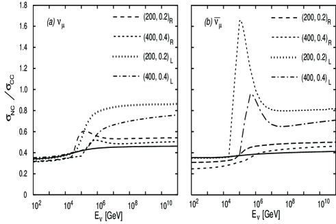
FIG. 1.: Neutral-current to charged-current ratios for (a) $\nu_{\mu}N$ and (b) $\overline{\nu}_{\mu}N$ interactions. The solid lines show the predictions of the standard model. The dashed (short-dashed) curves include the contributions of a right-handed squark, $\tilde{d}^{k}_{\mathrm{R}}$, with mass $\widetilde{m}=200~{}(400)~{}{\rm GeV}$ and coupling $\lambda^{\prime}_{21k}=0.2~{}(0.4)$. The dotted (dot-dashed) curves include the contributions of a left-handed squark, $\tilde{d}^{k}_{\mathrm{L}}$, for the same masses and couplings.

We see that the modifications from the standard-model cross sections are appreciable, even away from the resonance bump.

What about neutrino interactions on electron targets? In the standard model, because of the smallness of the electron-mass, neutrino-electron interactions in matter are weaker than neutrino-nucleon interactions, with the exception of the resonant formation of the intermediate boson in $\overline{\nu}_{e}e\rightarrow W^{-}$ interactions [45]. Additional effects may arise through $R$-violating interactions [43]. Because the $LL\overline{E}$ couplings are constrained to be small, only channels that involve resonant slepton production can display sizeable effects. Such couplings are too small to explain the Super-Kamiokande data in the framework of [42], nevertheless it is interesting to investigate whether they could have any observable effect. Small couplings result in small decay widths, and consequently, it will be difficult to separate such a narrow structure from the standard-model background. One interesting characteristic is that the slepton resonance will only be produced in downward-going interactions. Indeed, in water-equivalent units, the interaction length is given by

$$L_{\mathrm{int}}^{(e)}=\frac{1}{\sigma(E_{\nu})(10/18)N_{\mathrm{A}}}\;$$ (139)

where $N_{\mathrm{A}}$ is the Avogadro’s number and $(10/18)N_{\mathrm{A}}$ is the number of electrons in a mole of water. At the peak of a 200 (400) GeV slepton resonance produced in $\overline{\nu}e$ interactions, the interaction length indicates that the resonance is effectively extinguished for neutrinos that traverse the Earth.

Still, it would be easier to observe a slepton resonance in the case where the produced final states clearly stand out above the background. One such possibility arises if many $R$-violating couplings are simultaneously large, thus leading to exotic final-state topologies. An even better possibility arises if neutralinos are relatively light. In this case, the slepton may also decay into the corresponding lepton and a light neutralino, which in its turn decays into leptons and neutrinos:

$$\begin{array}[]{r c l}\nu_{\mu}e^{-}_{\mathrm{L}}\rightarrow\tilde{\tau}^{-}_{\mathrm{R}}&\rightarrow&\tau^{-}\tilde{\chi}^{0}\\ &&\phantom{\;\tau^{-}}\>\raisebox{4.73611pt}{\hbox to0.0pt{$|$\hss}}\!\rightarrow\tau^{+}_{\mathrm{R}}\nu_{e}\mu^{-}_{\mathrm{L}}\hbox{ or }\tau^{+}_{\mathrm{R}}\nu_{\mu}e^{-}_{\mathrm{L}}\end{array}$$ (140)

and

$$\begin{array}[]{r c l}\overline{\nu_{e,\mu}}e^{-}_{\mathrm{R}}\rightarrow\tilde{\tau}^{-}_{\mathrm{L}}\rightarrow&\rightarrow&\tau^{-}\tilde{\chi}^{0}\\ &&\phantom{\;\tau^{-}}\>\raisebox{4.73611pt}{\hbox to0.0pt{$|$\hss}}\!\rightarrow\tau^{+}_{\mathrm{L}}\overline{\nu}e^{-}_{\mathrm{R}}\end{array}$$ (141)

The decay length of a 1-PeV $\tau$ is about 50 m, so the production and subsequent decay of a $\tau$ at UHE will result in a characteristic “double-bang” signature in a Cherenkov detector. Because there are no conventional astrophysical sources of tau-neutrinos, while $\tau$-production through a slepton resonance with a mass $\geq$ 200 GeV, is essentially background-free, reactions that produce final-state $\tau$-leptons are of special interest for probing new physics.

VIII Summary and Conclusions

We discussed aspects of neutrino masses and lepton-number violation, in the light of the observations by Super-Kamiokande. We first studied phenomenological textures which match the data from various experiments and then investigated how such structures may arise, in models with flavour and GUT symmetries. In supersymmetric extensions of the Standard Model, renormalisation group effects were found to be important. In particular, for small $\tan\beta$, $b$–$\tau$ unification requires the presence of significant $\mu$–$\tau$ flavour mixing. On the other hand, for large $\tan\beta$, very small mixing at the GUT scale may be amplified to maximal mixing at low energies, and vice versa. Leptogenesis may give additional constraints on neutrino mass textures. Channels to directly search for lepton-number violation in ultra-high energy neutrino interactions, have also been proposed.

- [1] Y. Fukuda et al., Super-Kamiokande collaboration, Phys. Lett. B433 (1998) 9; Phys. Lett. B436 (1998) 33; Phys. Rev. Lett. 81 (1998) 1562.
- [2] S. Hatakeyama et al., Kamiokande collaboration, Phys. Rev. Lett. 81 (1998) 2016; M. Ambrosio et al., MACRO collaboration, Phys. Lett. B434 (1998) 451.
- [3] M. Apollonio et al., CHOOZ collaboration, Phys. Lett. B420 (1998) 397.
- [4] See for example, L. Wolfenstein, Phys. Rev. D17 (1978) 20; S. P. Mikheyev and A. Yu Smirnov, Yad. Fiz. 42 (1985) 1441; Sov. J. Nucl. Phys. 42, 913 (1986).
- [5] C. Athanassopoulos et al., LSND Collaboration; Phys. Rev. C54 (1996) 2685; Phys. Rev. Lett. 77 (1996) 3082; Phys. Rev. Lett. 81 (1998) 1774.
- [6] K. Eitel et al., Nucl. Phys. Proc. Suppl. 70 (1999) 210.
- [7] M. Gell-Mann, P. Ramond and R. Slansky, proceedings of the Supergravity Stony Brook Workshop, New York, 1979, eds. P. Van Nieuwenhuizen and D. Freedman (North-Holland, Amsterdam).
- [8] Z. Maki, M. Nakagawa and S. Sakata, Prog. Theor. Phys. 28 (1962) 247.
- [9] G.K. Leontaris, S. Lola and G.G. Ross, Nucl. Phys. B454 (1995) 25.
- [10] S. Lola and G.G.Ross, hep-ph/9902283; G.G. Ross, these proceedings.
- [11] K.S. Babu, J.C. Pati and F. Wilczek, hep-ph/9812538.
- [12] G.K. Leontaris and S. Lola, hep-ph/9510340, 1995 Corfu proceedings.
- [13] See for example the work by G. Altarelli and F. Feruglio, Phys. Lett. B439 (1998) 112; JHEP 9811 (1998) 021.
- [14] G.K. Leontaris, S. Lola, C. Scheich and J.D. Vergados, Phys. Rev. D 53 (1996) 6381; S. Lola and J.D. Vergados, Progr. Part. Nucl. Phys. 40 (1998) 71.
- [15] J. Ellis, G.K. Leontaris, S. Lola and D.V. Nanopoulos, hep-ph/9808251, to appear in Eur. J. Phys. C.
- [16] See for example: A. Joshipura and A. Smirnov, Phys. Lett. B439 (1998) 103; V. Barger et al., Phys. Lett. B437 (1998) 107; S.F. King, Phys. Lett. B439 (1998) 350; B.C. Allanach, hep-ph/9806294; R. Barbieri, L.J. Hall et al., hep-ph/9807235; G. Lazarides and N. Vlachos, Phys. Lett. B441 (1998) 46; M. Jezabek and Y. Sumino, Phys. Lett. B440(1998) 327; V. Barger, T. Weiler and K. Whisnant, Phys. Lett. B440 (1998) 1; E. Ma, Phys. Lett. B442 (1998) 238; Q. Shafi and Z. Tavartkiladze, hep-ph/9811282; F. Vissani, JHEP 9811 (1998) 025; C.H. Albright, K.S. Babu and S.M. Barr, Phys. Rev. Lett. 81 (1998) 1167; J. K. Elwood, N. Irges and P. Ramond, Phys. Rev. Lett. 81 (1998) 5064; M. Fukugita, M. Taminoto and T. Yanagida, hep-ph/9809554; W. Buchmüller and T. Yanagida, hep-ph/9810308; Y. Grossman, Y. Nir and Y. Shadmi, JHEP 9810 (1998) 007; C.D. Froggatt, M. Gibson and H.B. Nielsen, hep-ph/9811265; Z. Berezhiani and A. Rossi, hep-ph/9811447; C. Wetterich, hep-ph/9812426; R. Barbieri, L.J. Hall, G.L. Kane and G.G. Ross, hep-ph/9901228.
- [17] F. Vissani and A. Yu. Smirnov, Phys. Lett. B341 (1994) 173; A. Brignole, H. Murayama and R. Rattazzi, Phys. Lett. B335 (1994) 345.
- [18] L. Hall et al., Phys. Rev. D50 (1994) 7048;
- [19] M. Carena et al., Nucl. Phys. B426 (1994) 269.
- [20] E.G. Floratos, G.K. Leontaris and S. Lola, Phys. Lett. B365 (1996) 149.
- [21] K. Babu, C. N. Leung and J. Pantaleone, Phys. Lett. B319 (1993) 191.
- [22] P.H. Chankowski and Z. Pluciennik, Phys. Lett. B316 (1993) 312; M. Tanimoto, Phys. Lett. B360 (1995) 41.
- [23] C. D. Froggatt and H. B. Nielsen, Nucl. Phys. B147 (1979) 277.
- [24] The literature on the subject is vast. Some of the earlier references are: H. Fritzsch, Phys. Lett. 70B (1977) 436; B73 (1978) 317; Nucl. Phys. B155 (1979) 189; J. Harvey, P. Ramond and D. Reiss, Phys. Lett. B92 (1980) 309; S. Dimopoulos, L. J. Hall and S. Raby, Phys. Rev. Lett. 68 (1992) 1984; C. Wetterich, Nucl. Phys. B261 (1985) 461.
- [25] G.K. Leontaris and D.V. Nanopoulos, Phys. Lett. B212 (1988) 327; Y.Achiman and T. Greiner, Phys. Lett. B329 (1994) 33; Y. Grossman and Y. Nir, Nucl. Phys. B448 (1995) 30; P. Binétruy, S. Lavignac and P. Ramond, Nucl. Phys. B477 (1996) 353; P. Binétruy et al, Nucl. Phys. B496 (1997) 3.
- [26] L. Ibanez and G.G. Ross, Phys. Lett. B332 (1994) 100.
- [27] G. Altarelli and F. Feruglio, hep-ph/9812475.
- [28] J. Ellis, S. Lola and G.G. Ross, Nucl. Phys. B526 (1998) 115.
- [29] G.K. Leontaris and N.D. Tracas, Phys. Lett. B419 (1998) 206 and Phys. Lett. B431 (1998) 90; M. Gomez et al., hep-ph/9810291, to appear in Phys. Rev. D. Also see M. Gomez, these proceedings.
- [30] H. Dreiner et al., Nucl. Phys. B436 (1995) 461.
- [31] J. Pati and A. Salam, Phys. Rev. D10 (1974) 275.
- [32] B.C. Allanach et al, Phys. Rev. D56 (1997) 2632; Phys. Lett. B407 (1997) 275.
- [33] I. Antoniadis, J. Ellis, J. Hagelin and D.V. Nanopoulos, Phys. Lett. B194 (1987) 231; Phys. Lett. B231 (1989) 65.
- [34] J. Ellis, G.K. Leontaris, S. Lola and D.V. Nanopoulos, Phys. Lett. B425 (1998) 86.
- [35] M. Fukugita and T. Yanagida, Phys. Lett. B174 (1986) 45.
- [36] V.A. Kuzmin, V.A. Rubakov and M.E. Shaposhnikov, Phys. Lett. B155 (1985) 36.
- [37] J. Ellis, S. Lola and D.V. Nanopoulos, hep-ph/9902364.
- [38] See for instance A. Pilaftsis, hep-ph/9812256 and references therein. For the supersymmetric case, see L. Covi, E. Roulet and F. Vissani, Phys. Lett. B384 (1996) 169.
- [39] E.W. Kolb and M.S. Turner, The Early Universe, Frontiers in Physics by Addison-Wesley, New York.
- [40] See for example: M.A. Luty, Phys. Rev. D45 (1992) 455; M. Plumacher, Z. Phys. C74 (1997) 549; W. Buchmüller and M. Plumacher, Phys. Lett. B389 (1996) 73; J. Faridani et al., hep-ph/9804261, to appear in the Eur. J. Phys. C; M. Flanz and E.A. Paschos, Phys. Rev. D58 (1998) 113009.
- [41] V. Barger et al., hep-ph/9810121; G.L. Fogli et al., hep-ph/9902267.
- [42] M.C. Gonzalez-Garcia et al., hep-ph/9809531.
- [43] M. Carena, D. Choudhury, S. Lola and C. Quigg, Phys. Rev. D58 (1998) 095003.
- [44] For recent reviews, see G. Bhattacharyya, hep-ph/9709395; H. Dreiner, hep-ph/9707435.
- [45] R. Gandhi et al., Astropart. Phys. 5 (1996) 81.
- [46] H. Lai et. al., CTEQ Collaboration, Phys. Rev. D51(1995) 4763.