Exclusive $B\rightarrow K^{*}l^{+}l^{-}$ decay in the three Higgs doublet model

Abstract

We study the differential Branching ratio and $CP$ asymmetry for the exclusive decay $B\rightarrow K^{*}l^{+}l^{-}$ in the three Higgs doublet model with additional global $O(2)$ symmetry in the Higgs sector. We analyse dilepton mass square $q^{2}$ dependency of the these quantities. Further, we study the effect of new parameter of the global symmetry in the Higgs sector on the differential branching ratio and $CP$ asymmetry. We see that there exist an enhancement in the branching ratio and a considerable $CP$ violation for the relevant process. In addition to this, we realize that fixing dilepton mass gives information about the sign of the Wilson coefficient $C_{7}^{eff}$.Therefore, the future measurements of the CP asymmetry for $B\rightarrow K^{*}l^{+}l^{-}$ decay will give a powerful information about the sign of Wilson coefficient $C_{7}^{eff}$ and new physics beyond the SM.

1 Introduction

Measurement of the physical quantities for rare B-decays provides sensitive tests for the Standard model (SM) and it plays an important role in the determination of the parameters, such as Cabbibo-Kobayashi-Maskawa (CKM) matrix elements, leptonic decay constants, etc., since these decays are induced by flavor changing neutral currents (FCNC) at loop level in the SM. Further, they give a comprehensive information in the search of the physics beyond the SM, such as, two Higgs Doublet model (2HDM), Minimal Supersymmetric extension of the SM (MSSM) [1], etc. From the experimental point of view, the physical quantities, like Branching ratio ($Br$), $CP$ asymmetry ($A_{CP}$), forward backward asymmetry ($A_{FB}$), in rare B-decays have an outstanding role to obtain restrictions for the free parameters of the theory under consideration.

Among the rare B-decays, $B\rightarrow K^{*}l^{+}l^{-}$, induced by the inclusive process $b\rightarrow sl^{+}l^{-}$, has a large $Br$ in the framework of the SM and it can be measured in future experiments. Therefore, the study on this process becomes attractive. In the literature, there are various studies on these decays in the framework of the SM, 2HDM and MSSM [2]- [16].

$CP$ violating effect is another physical quantity which can give information about the free parameters of the model. For $B\rightarrow K^{*}l^{+}l^{-}$ decay, $CP$ violation almost vanishes in the framework of the SM, since the matrix element of the inclusive decay $b\rightarrow sl^{+}l^{-}$, inducing $B\rightarrow K^{*}l^{+}l^{-}$ process, contains only $V_{tb}V_{ts}^{*}$, due to the unitarity of CKM, $V_{ib}V_{is}^{*}=0\,\,,(i=u,c,t)$ and smallness of the term $V_{ub}V_{us}^{*}$. This problem was studied in the general 2HDM, so called model III, which has a new source for $CP$ violation [17]. In that work, the Yukawa couplings are taken complex and extra phase angles appear. These new parameters produce a considerable $CP$ violation effect for the decay under consideration.

In this work, we study $Br$ and $A_{CP}$ for the exclusive decay $B\rightarrow K^{*}l^{+}l^{-}$ in the framework of the three Higgs doublet model. Similar to the model III, complex Yukawa couplings are possible $CP$ violating sources. However, in the 3HDM, the number of free parameters are large compared to that of 2HDM since the Higss sector is extended. We solve this problem by introducing a new global $O(2)$ symmetry in the Higgs sector.

Even if the theoretical analysis of exclusive decays is more complicated due to the hadronic form factors, the experimental investigation of them is easier compared those of inclusive ones. Therefore, this work is devoted to the study of the exclusive $B\rightarrow K^{*}l^{+}l^{-}$ decay.

The paper is organized as follows: In Section 2, we present our theoretical work based on 3HDM and the matrix element for the inclusive $b\rightarrow sl^{+}l^{-}\,\,(l=e,\mu)$ decay in this model. In Section 3, we calculate $Br$ and $A_{CP}$ for the exclusive decay $B\rightarrow K^{*}l^{+}l^{-}$. Section 4 is devoted to discussion and our conclusions. In Appendix, we give some theoretical results for the 3HDM and explicit forms of the necessary functions appear in the text.

2 The inclusive $b\rightarrow sl^{+}l^{-}$ decay in the framework of 3HDM

In this section, we will derive the matrix element of the inclusive decay $b\rightarrow sl^{+}l^{-}$ ($l=e,\mu$), which induces the exclusive $B\rightarrow K^{*}l^{+}l^{-}$ process, in the framework of the 3HDM. We start with the general Yukawa interaction,

$${\cal{L}}_{Y} = \eta^{U}_{ij}\bar{Q}_{iL}\tilde{\phi_{1}}U_{jR}+\eta^{D}_{ij}\bar{Q}_{iL}\phi_{1}D_{jR}+\xi^{U}_{ij}\bar{Q}_{iL}\tilde{\phi_{2}}U_{jR}+\xi^{D}_{ij}\bar{Q}_{iL}\phi_{2}D_{jR}$$ (1)

$$+ \rho^{U}_{ij}\bar{Q}_{iL}\tilde{\phi_{3}}U_{jR}+\rho^{D}_{ij}\bar{Q}_{iL}\phi_{3}D_{jR}+h.c.\,\,\,,$$

where $L$ and $R$ denote chiral projections $L(R)=1/2(1\mp\gamma_{5})$, $\phi_{i}$ for $i=1,2,3$, are three scalar doublets and $\eta^{U,D}_{ij}$, $\xi^{U,D}_{ij}$, $\rho^{U,D}_{ij}$ are the Yukawa matrices having complex entries, in general. Now, we choose scalar Higgs doublets such that the first one describes only the SM part and last two carry the information about new physics beyond the SM:

$$\phi_{1}=\frac{1}{\sqrt{2}}\left[\left(\begin{array}[]{c c}0\\ v+H^{0}\end{array}\right)\;+\left(\begin{array}[]{c c}\sqrt{2}\chi^{+}\\ i\chi^{0}\end{array}\right)\right]\,,$$ (6)

(7)

$$\phi_{2}=\frac{1}{\sqrt{2}}\left(\begin{array}[]{c c}\sqrt{2}H^{+}\\ H^{1}+iH^{2}\end{array}\right)\,\,,\,\,\phi_{3}=\frac{1}{\sqrt{2}}\left(\begin{array}[]{c c}\sqrt{2}F^{+}\\ H^{3}+iH^{4}\end{array}\right)\,\,,$$ (12)

with the vacuum expectation values,

$$<\phi_{1}>=\frac{1}{\sqrt{2}}\left(\begin{array}[]{c c}0\\ v\end{array}\right)\,\,;<\phi_{2}>=0\,\,;<\phi_{3}>=0\,\,.$$ (15)

Note that, the similar choice was done in the literature for the general 2HDM [18]. The Yukawa interaction due to the new physics beyond the SM part is responsible for the Flavor Changing (FC) interactions and it can be written as

$${\cal{L}}_{Y,FC}=\xi^{U}_{ij}\bar{Q}_{iL}\tilde{\phi_{2}}U_{jR}+\xi^{D}_{ij}\bar{Q}_{iL}\phi_{2}D_{jR}+\rho^{U}_{ij}\bar{Q}_{iL}\tilde{\phi_{3}}U_{jR}+\rho^{D}_{ij}\bar{Q}_{iL}\phi_{3}D_{jR}+h.c.\,\,.$$ (16)

Here, the couplings $\xi^{U,D}$ and $\rho^{U,D}$ for the charged FC interactions are

$$\xi^{U}_{ch} = \xi_{N}\,\,V_{CKM}\,\,,$$

$$\xi^{D}_{ch} = V_{CKM}\,\,\xi_{N}\,\,,$$

$$\rho^{U}_{ch} = \rho_{N}\,\,V_{CKM}\,\,,$$

$$\rho^{D}_{ch} = V_{CKM}\,\,\rho_{N}\,\,,$$ (17)

and

$$\xi^{U,D}_{N} = (V_{L}^{U,D})^{-1}\xi^{U,D}\,V_{R}^{U,D}\,\,,$$

$$\rho^{U,D}_{N} = (V_{L}^{U,D})^{-1}\rho^{U,D}\,V_{R}^{U,D}\,\,,$$ (18)

where the index ”$N$” in $\xi^{U,D}_{N}$ denotes the word ”neutral”.

At this stage, we obtain the effective Hamiltonian for the inclusive process $b\rightarrow sl^{+}l^{-}$ by matching the full theory with the effective low energy one at the high scale $\mu$. In this calculation, there are additional charged Higgs effects coming from the new charged Higgs particles $F^{\pm}$ (see eqs. (20) and (21)). Fortunately, $F^{\pm}-quark-quark$ interaction is the same as $H^{\pm}-quark-quark$ one except new Yukawa couplings and they give additional contributions to the Wilson coefficients withouth changing the operator basis $O_{i}(\mu)$ (see [16]). The Wilson coefficients are evaluated from $\mu$ down to the lower scale $\mu\sim O(m_{b})$ using the renormalization group equations. Here the problem is to choose the high scale. In the literature, this scale is taken as the mass of charged Higgs, $\mu=m_{H^{\pm}}$, in the 2HDM, since the evaluation from $\mu=m_{H^{\pm}}$ to $\mu=m_{W}$ gives negligible contribution to the Wilson coefficients( see [19]). In our case, there is a new charged Higgs $F^{\pm}$ and its mass $m_{F^{\pm}}$ can be greater compared to $m_{H^{\pm}}$. However, by introducing a new symmetry in the Higgs sector, we can take that masses of $F^{\pm}$ and $H^{\pm}$ are the same. Before starting with this discussion, we would like to present the effective Hamiltonian, obtained by integrating out the heavy degrees of freedom, here, $t$ quark, $W^{\pm}$, $H^{\pm}$, $F^{\pm}$, $H^{1}$, $H^{2}$, $H^{3}$ and $H^{4}$ where $H^{\pm}$, $F^{\pm}$ and $H^{1}$,$H^{2}$, $H^{3}$,$H^{4}$ denote charged and neutral Higgs bosons respectively:

$${\cal{H}}_{eff}=-4\frac{G_{F}}{\sqrt{2}}V_{tb}V^{*}_{ts}\sum_{i=1}^{12}(C_{i}(\mu)O_{i}(\mu)+C^{\prime}_{i}(\mu)O^{\prime}_{i}(\mu))\,\,.$$ (19)

In this equation, $O_{i}$ are current-current ($i=1,2,11,12$), penguin ($i=1,...6$), magnetic penguin ($i=7,8$) and semileptonic ($i=9,10$) operators [16, 20, 21] and primed counterparts are their flipped chirality partners [16]. $C_{i}(\mu)$ and $C^{\prime}_{i}(\mu)$ are Wilson coefficients renormalized at the scale $\mu$. The initial values of the Wilson coefficients in the SM model, $C_{i}^{(\prime)SM}(m_{W})$, can be found in Appendix A. The additional contributions to the initial values of the Wilson coefficients, due to two new Higgs scalars are denoted by $C_{i}^{H}(m_{W})$ and for unprimed set of operators we have

$$C^{H}_{1,\dots 6,11,12}(m_{W}) = 0\,\,,$$

$$C_{7}^{H}(m_{W}) = \frac{1}{m_{t}^{2}}\,(\bar{\xi}^{*U}_{N,tt}+\bar{\xi}^{*U}_{N,tc}\frac{V_{cs}^{*}}{V_{ts}^{*}})\,(\bar{\xi}^{U}_{N,tt}+\bar{\xi}^{U}_{N,tc}\frac{V_{cb}}{V_{tb}})F_{1}(y)\,\,$$

$$+ \frac{1}{m_{t}m_{b}}\,(\bar{\xi}^{*U}_{N,tt}+\bar{\xi}^{*U}_{N,tc}\frac{V_{cs}^{*}}{V_{ts}^{*}})\,(\bar{\xi}^{D}_{N,bb}+\bar{\xi}^{D}_{N,sb}\frac{V_{ts}}{V_{tb}})F_{2}(y)\,\,$$

$$+ \frac{1}{m_{t}^{2}}\,(\bar{\rho}^{*U}_{N,tt}+\bar{\rho}^{*U}_{N,tc}\frac{V_{cs}^{*}}{V_{ts}^{*}})\,(\bar{\rho}^{U}_{N,tt}+\bar{\rho}^{U}_{N,tc}\frac{V_{cb}}{V_{tb}})F_{1}(y^{\prime})\,\,$$

$$+ \frac{1}{m_{t}m_{b}}\,(\bar{\rho}^{*U}_{N,tt}+\bar{\rho}^{*U}_{N,tc}\frac{V_{cs}^{*}}{V_{ts}^{*}})\,(\bar{\rho}^{D}_{N,bb}+\bar{\rho}^{D}_{N,sb}\frac{V_{ts}}{V_{tb}})F_{2}(y^{\prime})\,\,,$$

$$C_{8}^{H}(m_{W}) = \frac{1}{m_{t}^{2}}\,(\bar{\xi}^{*U}_{N,tt}+\bar{\xi}^{*U}_{N,tc}\frac{V_{cs}^{*}}{V_{ts}^{*}})\,(\bar{\xi}^{U}_{N,tt}+\bar{\xi}^{U}_{N,tc}\frac{V_{cb}}{V_{tb}})G_{1}(y)\,\,$$

$$+ \frac{1}{m_{t}m_{b}}\,(\bar{\xi}^{*U}_{N,tt}+\bar{\xi}^{*U}_{N,tc}\frac{V_{cs}^{*}}{V_{ts}^{*}})\,(\bar{\xi}^{D}_{N,bb}+\bar{\xi}^{U}_{N,sb}\frac{V_{ts}}{V_{tb}})G_{2}(y)\,\,$$

$$+ \frac{1}{m_{t}^{2}}\,(\bar{\rho}^{*U}_{N,tt}+\bar{\rho}^{*U}_{N,tc}\frac{V_{cs}^{*}}{V_{ts}^{*}})\,(\bar{\rho}^{U}_{N,tt}+\bar{\rho}^{U}_{N,tc}\frac{V_{cb}}{V_{tb}})G_{1}(y^{\prime})\,\,$$

$$+ \frac{1}{m_{t}m_{b}}\,(\bar{\rho}^{*U}_{N,tt}+\bar{\rho}^{*U}_{N,tc}\frac{V_{cs}^{*}}{V_{ts}^{*}})\,(\bar{\rho}^{D}_{N,bb}+\bar{\rho}^{U}_{N,sb}\frac{V_{ts}}{V_{tb}})G_{2}(y^{\prime})\,\,,$$

$$C_{9}^{H}(m_{W}) = \frac{1}{m_{t}^{2}}\,(\bar{\xi}^{*U}_{N,tt}+\bar{\xi}^{*U}_{N,tc}\frac{V_{cs}^{*}}{V_{ts}^{*}})\,(\bar{\xi}^{U}_{N,tt}+\bar{\xi}^{U}_{N,tc}\frac{V_{cb}}{V_{tb}})H_{1}(y)\,\,$$

$$+ \frac{1}{m_{t}^{2}}\,(\bar{\rho}^{*U}_{N,tt}+\bar{\rho}^{*U}_{N,tc}\frac{V_{cs}^{*}}{V_{ts}^{*}})\,(\bar{\rho}^{U}_{N,tt}+\bar{\rho}^{U}_{N,tc}\frac{V_{cb}}{V_{tb}})H_{1}(y^{\prime})\,\,,$$

$$C_{10}^{H}(m_{W}) = \frac{1}{m_{t}^{2}}\,(\bar{\xi}^{*U}_{N,tt}+\bar{\xi}^{*U}_{N,tc}\frac{V_{cs}^{*}}{V_{ts}^{*}})\,(\bar{\xi}^{U}_{N,tt}+\bar{\xi}^{U}_{N,tc}\frac{V_{cb}}{V_{tb}})L_{1}(y)\,\,$$ (20)

$$+ \frac{1}{m_{t}^{2}}\,(\bar{\rho}^{*U}_{N,tt}+\bar{\rho}^{*U}_{N,tc}\frac{V_{cs}^{*}}{V_{ts}^{*}})\,(\bar{\rho}^{U}_{N,tt}+\bar{\rho}^{U}_{N,tc}\frac{V_{cb}}{V_{tb}})L_{1}(y^{\prime})\,\,,$$

and for primed set of operators,

$$C^{\prime H}_{1,\dots 6,11,12}(m_{W}) = 0\,\,,$$

$$C^{\prime H}_{7}(m_{W}) = \frac{1}{m_{t}^{2}}\,(\bar{\xi}^{*D}_{N,bs}\frac{V_{tb}}{V_{ts}^{*}}+\bar{\xi}^{*D}_{N,ss})\,(\bar{\xi}^{D}_{N,bb}+\bar{\xi}^{D}_{N,sb}\frac{V_{ts}}{V_{tb}})F_{1}(y)\,\,$$

$$+ \frac{1}{m_{t}m_{b}}\,(\bar{\xi}^{*D}_{N,bs}\frac{V_{tb}}{V_{ts}^{*}}+\bar{\xi}^{*D}_{N,ss})\,(\bar{\xi}^{U}_{N,tt}+\bar{\xi}^{U}_{N,tc}\frac{V_{cb}}{V_{tb}})F_{2}(y)\,\,$$

$$+ \frac{1}{m_{t}^{2}}\,(\bar{\rho}^{*D}_{N,bs}\frac{V_{tb}}{V_{ts}^{*}}+\bar{\rho}^{*D}_{N,ss})\,(\bar{\rho}^{D}_{N,bb}+\bar{\rho}^{D}_{N,sb}\frac{V_{ts}}{V_{tb}})F_{1}(y^{\prime})\,\,$$

$$+ \frac{1}{m_{t}m_{b}}\,(\bar{\rho}^{*D}_{N,bs}\frac{V_{tb}}{V_{ts}^{*}}+\bar{\rho}^{*D}_{N,ss})\,(\bar{\rho}^{U}_{N,tt}+\bar{\rho}^{U}_{N,tc}\frac{V_{cb}}{V_{tb}})F_{2}(y^{\prime})\,,$$

$$C^{\prime H}_{8}(m_{W}) = \frac{1}{m_{t}^{2}}\,(\bar{\xi}^{*D}_{N,bs}\frac{V_{tb}}{V_{ts}^{*}}+\bar{\xi}^{*D}_{N,ss})\,(\bar{\xi}^{D}_{N,bb}+\bar{\xi}^{D}_{N,sb}\frac{V_{ts}}{V_{tb}})G_{1}(y)\,\,$$

$$+ \frac{1}{m_{t}m_{b}}\,(\bar{\xi}^{*D}_{N,bs}\frac{V_{tb}}{V_{ts}^{*}}+\bar{\xi}^{*D}_{N,ss})\,(\bar{\xi}^{U}_{N,tt}+\bar{\xi}^{U}_{N,tc}\frac{V_{cb}}{V_{tb}})G_{2}(y)\,\,$$

$$+ \frac{1}{m_{t}^{2}}\,(\bar{\rho}^{*D}_{N,bs}\frac{V_{tb}}{V_{ts}^{*}}+\bar{\rho}^{*D}_{N,ss})\,(\bar{\rho}^{D}_{N,bb}+\bar{\rho}^{D}_{N,sb}\frac{V_{ts}}{V_{tb}})G_{1}(y^{\prime})\,\,$$

$$+ \frac{1}{m_{t}m_{b}}\,(\bar{\rho}^{*D}_{N,bs}\frac{V_{tb}}{V_{ts}^{*}}+\bar{\rho}^{*D}_{N,ss})\,(\bar{\rho}^{U}_{N,tt}+\bar{\rho}^{U}_{N,tc}\frac{V_{cb}}{V_{tb}})G_{2}(y^{\prime})\,,$$

$$C^{\prime H}_{9}(m_{W}) = \frac{1}{m_{t}^{2}}\,(\bar{\xi}^{*D}_{N,bs}\frac{V_{tb}}{V_{ts}^{*}}+\bar{\xi}^{*D}_{N,ss})\,(\bar{\xi}^{D}_{N,bb}+\bar{\xi}^{D}_{N,sb}\frac{V_{ts}}{V_{tb}})H_{1}(y)\,\,$$

$$+ \frac{1}{m_{t}^{2}}\,(\bar{\rho}^{*D}_{N,bs}\frac{V_{tb}}{V_{ts}^{*}}+\bar{\rho}^{*D}_{N,ss})\,(\bar{\rho}^{D}_{N,bb}+\bar{\rho}^{D}_{N,sb}\frac{V_{ts}}{V_{tb}})H_{1}(y^{\prime})\,\,,$$

$$C^{\prime H}_{10}(m_{W}) = \frac{1}{m_{t}^{2}}\,(\bar{\xi}^{*D}_{N,bs}\frac{V_{tb}}{V_{ts}^{*}}+\bar{\xi}^{D}_{N,ss})\,(\bar{\xi}^{D}_{N,bb}+\bar{\xi}^{D}_{N,sb}\frac{V_{ts}}{V_{tb}})L_{1}(y)$$ (21)

$$+ \frac{1}{m_{t}^{2}}\,(\bar{\rho}^{*D}_{N,bs}\frac{V_{tb}}{V_{ts}^{*}}+\bar{\rho}^{D}_{N,ss})\,(\bar{\rho}^{D}_{N,bb}+\bar{\rho}^{D}_{N,sb}\frac{V_{ts}}{V_{tb}})L_{1}(y^{\prime})\,\,,$$

where $y=m_{t}^{2}/m_{H^{\pm}}^{2}$ and $y^{\prime}=m_{t}^{2}/m_{F^{\pm}}^{2}$. In eqs. (20) and (21) we used the redefinition

$$\xi^{U,D}=\sqrt{\frac{4G_{F}}{\sqrt{2}}}\,\,\bar{\xi}^{U,D}\,\,.$$ (22)

The explicit forms of the functions $F_{1(2)}(y)$, $G_{1(2)}(y)$, $H_{1}(y)$ and $L_{1}(y)$ can be found in Appedix A. In the calculations, we neglect the contributions of the neutral Higgs bosons to the Wilson coefficient $C_{7}^{eff}$ (see [22]). Note that, the neutral Higgs bosons coming from $\phi_{3}$ give contribution to $C_{7}^{eff}$, including the Yukawa couplings $\bar{\rho}^{D}_{N,bj}$ and $\bar{\rho}^{D}_{N,is}$ ($j=d,s$  ;  $i=d,s,b$), similar to the ones coming from $\phi_{2}$ [22].

In the 3HDM model, the Higgs sector is extended and this leads to an increase in the number of free parameters, namely, masses of new charged and neutral Higgs particles, new Yukawa couplings. In the Appendix B, we give the general gauge and CP invariant Higgs potential for the 3HDM and present the masses of charged and neutral Higgs particles. Now, our aim is to decrease the number of free parameters in the model under consideration. We consider three Higgs scalars as orthogonal vectors in a new space, which we call Higgs flavor space and we denote the Higgs flavor index by ”$m$”, where $m=1,2,3$. We introduce a new global symmetry on the Higgs sector which keeps the 3HDM Lagrangian invariant. Let us take the following $O(2)$ transformation:

$$\phi^{\prime}_{1} = \phi_{1}\,\,,$$

$$\phi^{\prime}_{2} = cos\,\alpha\,\,\phi_{2}+sin\,\alpha\,\,\phi_{3}\,\,,$$

$$\phi^{\prime}_{3} = -sin\,\alpha\,\,\phi_{2}+cos\,\alpha\,\,\phi_{3}\,\,,$$ (23)

where $\alpha$ is the global parameter, which represents a rotation of the vectors $\phi_{2}$ and $\phi_{3}$ along the axis that $\phi_{1}$ lies, in the Higgs flavor space. The kinetic term of the Lagrangian (see Appendix B) is invariant under this transformation. The invariance of the potential term can be obtained if the following conditions on the free parameters (eq. 50) are satisfied:

$$c_{5}=c_{6}\,\,\,,c_{8}=c_{9}\,\,,c_{11}=c_{12}\,\,,$$

$$c_{2}=c_{3}=c_{7}=c_{10}=0\,\,,$$ (24)

and we get

$$V(\phi_{1},\phi_{2},\phi_{3}) = c_{1}(\phi_{1}^{+}\phi_{1}-v^{2}/2)^{2}+c_{4}[(\phi_{1}^{+}\phi_{1}-v^{2}/2)^{2}+\phi_{2}^{+}\phi_{2}+\phi_{3}^{+}\phi_{3}]^{2}$$ (25)

$$+ c_{5}[(\phi_{1}^{+}\phi_{1})(\phi_{2}^{+}\phi_{2}+\phi_{3}^{+}\phi_{3})-(\phi_{1}^{+}\phi_{2})(\phi_{2}^{+}\phi_{1})-(\phi_{1}^{+}\phi_{3})(\phi_{3}^{+}\phi_{1})]$$

$$+ c_{8}([Re(\phi_{1}^{+}\phi_{2})]^{2}+[Re(\phi_{1}^{+}\phi_{3})]^{2})+c_{11}([Im(\phi_{1}^{+}\phi_{2})]^{2}+[Im(\phi_{1}^{+}\phi_{3})]^{2})$$

$$+ c_{13}[Im(\phi_{2}^{+}\phi_{3})]^{2}+c_{14}$$

Therefore, the masses of new particles are

$$m_{F^{\pm}}=m_{H^{\pm}}=c_{5}\frac{v^{2}}{2}\,\,,$$

$$m_{H^{3}}=m_{H^{1}}=c_{8}\frac{v^{2}}{2}\,\,,$$

$$m_{H^{4}}=m_{H^{2}}=c_{11}\frac{v^{2}}{2}\,\,,$$

(26)

It is the first gain in decreasing the number of free parameters. Now, we apply this transformation to the Yukawa Lagrangian (eq.(1)). This term is invariant if the transformed Yukawa matrices satisfy the expressions

$$\bar{\xi}^{\prime U(D)}_{ij} = \bar{\xi}^{U(D)}_{ij}cos\,\alpha+\bar{\rho}^{U(D)}_{ij}sin\,\alpha\,\,,$$

$$\bar{\rho}^{\prime U(D)}_{ij} = -\bar{\xi}^{U(D)}_{ij}sin\,\alpha+\bar{\rho}^{U(D)}_{ij}cos\,\alpha\,\,.$$ (27)

and therefore

$$(\bar{\xi}^{\prime U(D)})^{+}\bar{\xi}^{\prime U(D)}+(\bar{\rho}^{\prime U(D)})^{+}\bar{\rho}^{\prime U(D)}=(\bar{\xi}^{U(D)})^{+}\bar{\xi}^{U(D)}+(\bar{\rho}^{U(D)})^{+}\bar{\rho}^{U(D)}\,\,,$$ (28)

which permits us to parametrize the Yukawa matrices $\bar{\xi}^{U(D)}$ and $\bar{\rho}^{U(D)}$ as

$$\bar{\xi}^{U(D)}=\epsilon^{U(D)}cos\,\theta\,\,,$$

$$\bar{\rho}^{U}=\epsilon^{U}sin\,\theta\,\,,$$

$$\bar{\rho}^{D}=i\epsilon^{D}sin\,\theta\,\,,$$ (29)

where $\epsilon^{U(D)}$ are real matrices satisfy the equation

$$(\bar{\xi}^{\prime U(D)})^{+}\bar{\xi}^{\prime U(D)}+(\bar{\rho}^{\prime U(D)})^{+}\bar{\rho}^{\prime U(D)}=(\epsilon^{U(D)})^{T}\epsilon^{U(D)}$$ (30)

Here $T$ denotes transpose operation. In eq. (29), we take $\bar{\rho^{D}}$ complex to carry all $CP$ violating effects on the third Higgs scalar.

Finally, we could reduce the number of free parameters, here the Yukawa matrices $\bar{\xi}^{U,(D)}$ and $\bar{\rho}^{U,(D)}$, by connecting them by the expression given in eq. (29). Further, we take into account only the Yukawa couplings $\bar{\xi}^{U}_{N,tt}$, $\bar{\xi}^{D}_{N,bb}$, $\bar{\rho}^{U}_{N,tt}$ and $\bar{\rho}^{D}_{N,bb}$, since we assume that the others are small due to the discussion given in [16]. Now, we rewrite the contributions of the charged Higgs particles to the initial values of the Wilson coefficients as:

$$C^{H}_{1,\dots 6,11,12}(m_{W}) = 0\,\,,$$

$$C_{7}^{H}(m_{W}) = \frac{1}{m_{t}^{2}}\,(\bar{\xi}^{*U}_{N,tt}\,\bar{\xi}^{U}_{N,tt}+\bar{\rho*}^{U}_{N,tt}\,\bar{\rho}^{U}_{N,tt})F_{1}(y)$$

$$+ \frac{1}{m_{t}m_{b}}\,(\bar{\xi}^{*U}_{N,tt}\,\bar{\xi}^{D}_{N,bb}+\bar{\rho}^{*U}_{N,tt}\,\bar{\rho}^{D}_{N,bb})F_{2}(y)\,\,,$$

$$C_{8}^{H}(m_{W}) = \frac{1}{m_{t}^{2}}\,(\bar{\xi}^{*U}_{N,tt}\,\bar{\xi}^{U}_{N,tt}+\bar{\rho}^{*U}_{N,tt}\,\bar{\rho}^{U}_{N,tt})G_{1}(y)$$

$$+ \frac{1}{m_{t}m_{b}}\,(\bar{\xi}^{*U}_{N,tt}\bar{\xi}^{D}_{N,bb}+\bar{\rho}^{*U}_{N,tt}\bar{\rho}^{D}_{N,bb})G_{2}(y)\,\,,$$

$$C_{9}^{H}(m_{W}) = \frac{1}{m_{t}^{2}}\,(\bar{\xi}^{*U}_{N,tt}\bar{\xi}^{U}_{N,tt}+\bar{\rho}^{*U}_{N,tt}\bar{\rho}^{U}_{N,tt})H_{1}(y)\,\,,$$

$$C_{10}^{H}(m_{W}) = \frac{1}{m_{t}^{2}}\,(\bar{\xi}^{*U}_{N,tt}\bar{\xi}^{U}_{N,tt}+\bar{\rho}^{*U}_{N,tt}\bar{\rho}^{U}_{N,tt})L_{1}(y)\,\,,$$ (31)

and neglect the primed coefficients since they include small Yukawa couplings. Here, $\bar{\xi}^{U(D)}_{N,tt(bb)}$ and $\bar{\rho}^{U(D)}_{N,tt(bb)}$ can be obtained by using eq. (29). Note that, with the replacements $\bar{\xi}^{*U}_{N,tt}\bar{\xi}^{U}_{N,tt}+\bar{\rho}^{*U}_{N,tt}\bar{\rho}^{U}_{N,tt}\rightarrow\bar{\xi}^{*U}_{N,tt}\bar{\xi}^{U}_{N,tt}$ and $\bar{\xi}^{*U}_{N,tt}\bar{\xi}^{D}_{N,bb}+\bar{\rho}^{*U}_{N,tt}\bar{\rho}^{D}_{N,bb}\rightarrow\bar{\xi}^{*U}_{N,tt}\bar{\xi}^{D}_{N,bb}$  we get the results for the general 2HDM (model III) [16]. By neglecting the primed ones , the initial values of the Wilson coefficients can be written as

$$C_{i}^{3HDM}(m_{W}) = C_{i}^{SM}(m_{W})+C_{i}^{H}(m_{W})\,\,,$$ (32)

and using these initial values, we can calculate the coefficients $C_{i}^{3HDM}(\mu)$ at any lower scale with five quark effective theory, namely $u,c,d,s,b$. In the process under consideration the Wilson coefficients $C_{7}^{eff}(\mu)$, $C_{9}^{eff}(\mu)$ and $C_{10}(\mu)$ play the important role in the physical quantities and the others enter into expressions with operator mixing. Besides the perturbative part, there exist the long distance (LD) effects due to the real $\bar{c}c$ in the intermediate states, i.e. the cascade process $B\rightarrow K^{*}\psi_{i}\rightarrow K^{*}l^{+}l^{-}$ where $i=1,..,6$. These effects appear in the Wilson coefficient $C_{9}^{eff}$ and using a Breit-Wigner form of the resonance propagator [13, 23], they are added to the perturbative one coming from the $c\bar{c}$ loop:

$$C_{9}^{eff}(\mu)=C_{9}^{pert}(\mu)+Y_{reson}\,\,,$$ (33)

where $Y_{reson}$ in NDR scheme is defined as

$$Y_{reson} = -\frac{3}{\alpha^{2}_{em}}\kappa\sum_{V_{i}=\psi_{i}}\frac{\pi\Gamma(V_{i}\rightarrow ll)m_{V_{i}}}{q^{2}-m^{2}_{V_{i}}+im_{V_{i}}\Gamma_{V_{i}}}$$ (34)

$$\left(3C_{1}(\mu)+C_{2}(\mu)+3C_{3}(\mu)+C_{4}(\mu)+3C_{5}(\mu)+C_{6}(\mu)\right).$$

In eqs. (34), the phenomenological parameter $\kappa$ is taken as $\kappa=2.3$ [10]. The explicit forms of the perturbative parts of the Wilson coefficients $C_{i}(\mu)\,\,,i=1,...,9$ including NLO QCD corrections can be found in the literature [16, 24, 25].

Finally, neglecting the strange quark mass and primed coefficients, the matrix element for $b\rightarrow s\ell^{+}\ell^{-}$ decay is obtained as:

$${\cal M} = -\frac{G_{F}\alpha_{em}}{2\sqrt{2}\pi}V_{tb}V^{*}_{ts}\Bigg{\{}\,C_{9}^{eff}(\mu)\,\bar{s}\gamma_{\mu}(1-\gamma_{5})b\,\,\bar{\ell}\gamma^{\mu}\ell+C_{10}(\mu)\,\bar{s}\gamma_{\mu}(1-\gamma_{5})b\,\,\bar{\ell}\gamma^{\mu}\gamma_{5}\ell$$

$$- 2C^{eff}_{7}(\mu)\,\frac{m_{b}}{q^{2}}\,\bar{s}i\sigma_{\mu\nu}q^{\nu}(1+\gamma_{5})b\,\,\bar{\ell}\gamma^{\mu}\ell\Bigg{\}}~{}.$$

3 The exclusive $B\rightarrow K^{*}l^{+}l^{-}$ decay

In this section, we study the Branching ratio (Br) and the CP asymmetry ($A_{CP}$) of the exclusive decay $B\rightarrow K^{*}l^{+}l^{-}$ in the 3HDM. Using the results for the matrix elements $\langle K^{*}\left|\bar{s}\gamma_{\mu}(1\pm\gamma_{5})b\right|B\rangle$, and $\langle K^{*}\left|\bar{s}i\sigma_{\mu\nu}q^{\nu}(1\pm\gamma_{5})b\right|B\rangle$ [26], the hadronic matrix element of the $B\rightarrow K^{*}l^{+}l^{-}$ decay is obtained as [27]:

$${\cal M} = -\frac{G\alpha_{em}}{2\sqrt{2}\pi}V_{tb}V_{ts}^{*}\Bigg{\{}\bar{\ell}\gamma^{\mu}\ell\left[2A\epsilon_{\mu\nu\rho\sigma}\epsilon^{*\nu}p_{K^{*}}^{\rho}q^{\sigma}+iB_{1}\epsilon^{*}_{\mu}-iB_{2}(\epsilon^{*}q)(p_{B}+p_{K^{*}})_{\mu}-iB_{3}(\epsilon^{*}q)q_{\mu}\right]$$ (35)

$$+ \bar{\ell}\gamma^{\mu}\gamma_{5}\ell\left[2C\epsilon_{\mu\nu\rho\sigma}\epsilon^{*\nu}p_{K^{*}}^{\rho}q^{\sigma}+iD_{1}\epsilon^{*}_{\mu}-iD_{2}(\epsilon^{*}q)(p_{B}+p_{K^{*}})_{\mu}-iD_{3}(\epsilon^{*}q)q_{\mu}\right]\Bigg{\}}~{},$$

where $\epsilon^{*\mu}$ is the polarization vector of $K^{*}$ meson, $p_{B}$ and $p_{K^{*}}$ are four momentum vectors of $B$ and $K^{*}$ mesons, $q=p_{B}-p_{K^{*}}$ and $A$, $C$, $B_{i}$, and $D_{i}$ $i=1,2,3$ are the form factors of the relevant process. Their explicit forms can be found in the Appendix C.

Using eq.(35), we get the double differential decay rate:

$$\frac{d\Gamma}{dq^{2}dz} = \frac{G^{2}\alpha_{em}^{2}\left|V_{tb}V_{ts}^{*}\right|^{2}\lambda^{1/2}}{2^{12}\pi^{5}m_{B}}\Bigg{\{}2\lambda m_{B}^{4}\Bigg{[}m_{B}^{2}s(1+z^{2})\left(\left|A\right|^{2}+\left|C\right|^{2}\right)\Bigg{]}$$ (36)

$$+ \frac{\lambda m_{B}^{4}}{2r}\Bigg{[}\lambda m_{B}^{2}(1-z^{2})\left(\left|B_{2}\right|^{2}+\left|D_{2}\right|^{2}\right)\Bigg{]}$$

$$+ \frac{1}{2r}\Bigg{[}m_{B}^{2}\left\{\lambda(1-z^{2})+8rs\right\}\left(\left|B_{1}\right|^{2}+\left|D_{1}\right|^{2}\right)$$

$$- 2\lambda m_{B}^{4}(1-r-s)(1-z^{2})\left\{Re\left(B_{1}B_{2}^{*}\right)+Re\left(D_{1}D_{2}^{*}\right)\right\}\Bigg{]}$$

$$- 8m_{B}^{4}s\lambda^{1/2}z\Bigg{[}\left\{Re\left(B_{1}C^{*}\right)+Re\left(AD_{1}^{*}\right)\right\}\Bigg{]}\Bigg{\}}~{},$$

where $z=cos\beta$ , $\beta$ is the angle between the momentum of $\ell$ lepton and that of $B$ meson in the center of mass frame of the lepton pair, $\lambda=1+r^{2}+s^{2}-2r-2s-2rs$, $r=\frac{\displaystyle{m_{K^{*}}^{2}}}{\displaystyle{m_{B}^{2}}}$ and $s=\frac{\displaystyle{q^{2}}}{\displaystyle{m_{B}^{2}}}$.

$A_{CP}$ is another important physical quantity which almost does not exist for the given process in the framework of the SM. However, with the choice of the complex Yukawa couplings, it is possible that such asymmetry exists, in extended models like 2HDM [17]. In our case, the model under consideration is the 3HDM with global $O(2)$ symmetry in the Higgs sector and the possible source of CP violation comes from complex Yukawa couplings in the third Higgs doublet. Using the definition of $A_{CP}$

$$A_{CP}=\frac{\frac{d\Gamma(\bar{B_{s}}\rightarrow K^{*}e^{+}e^{-})}{dq^{2}}-\frac{d\Gamma(B_{s}\rightarrow\bar{K^{*}}e^{+}e^{-})}{dq^{2}}}{\frac{d\Gamma(\bar{B_{s}}\rightarrow K^{*}e^{+}e^{-})}{dq^{2}}+\frac{d\Gamma(B_{s}\rightarrow\bar{K^{*}}e^{+}e^{-})}{dq^{2}}}\,\,.$$ (37)

we get

$$A_{CP}=-2Im(\lambda_{2})\frac{Im(C_{9}^{eff}(\mu))\,\,P_{1}(\mu)\,\,\Delta}{Re(\lambda_{2})[-2(P_{1}(\mu)+2P_{2}(\mu))\,Re(C_{9}^{eff}(\mu))\,\Delta+\Omega}.$$ (38)

In eq. (38) we use the same parametrization as in [17]

$$C_{7}^{eff}(\mu)=P_{1}(\mu)\,\lambda_{2}+P_{2}(\mu)\,\,,$$ (39)

where $\lambda_{2}$ is

$$\lambda_{2}=\frac{1}{m_{t}\,m_{b}}\bar{\epsilon}^{U}_{N,tt}\bar{\epsilon}^{D}_{N,bb}(cos^{2}\,\theta+isin^{2}\,\theta)$$ (40)

Here the functions $P_{1}(\mu)$ and $P_{2}(\mu)$ can be written as the combinations of LO and NLO part, namely,

$$P_{1}(\mu) = P_{1}^{LO}(\mu)+P_{1}^{NLO}(\mu)\,\,,$$

$$P_{2}(\mu) = P_{2}^{LO}(\mu)+P_{2}^{NLO}(\mu)\,\,,$$ (41)

and

$$P_{1}^{LO}(\mu) = \eta^{16/23}F_{2}(y)+\frac{8}{3}(\eta^{14/23}-\eta^{16/23})\,G_{2}(y)$$

$$P_{2}^{LO}(\mu) = \eta^{16/23}[C_{7}^{SM}(m_{W})+\frac{|\bar{\epsilon}^{U}_{N,tt}|^{2}}{m_{t}^{2}}F_{1}(y)]$$ (42)

$$+ \frac{8}{3}(\eta^{14/23}-\eta^{16/23})[C_{8}^{SM}(m_{W})+\frac{|\bar{\epsilon}^{U}_{N,tt}|^{2}}{m_{t}^{2}}G_{1}(y)]$$

$$+ Q_{d}(C_{5}^{LO}(\mu)+N_{c}\,C_{6}^{LO}(\mu))+Q_{u}(\frac{m_{c}}{m_{b}}C_{12}^{LO}(\mu)+N_{c}\frac{m_{c}}{m_{b}}C_{11}^{LO}(\mu))$$

$$+ C_{2}(m_{W})\sum_{i=1}^{8}h_{i}\eta^{a_{i}}\,\,,$$

where $\eta=\frac{\alpha_{s}(\mu)}{\alpha_{s}(m_{W})}$, $h_{i}$ and $a_{i}$ are numbers appear during the evaluation [13]. $P_{1}^{NLO}(\mu)$ is the coefficient of $\lambda_{2}$ in the expression $\frac{\alpha_{s}(\mu)}{4\pi}C_{7}^{(1)\,3HDM}(\mu)$ and $P_{2}^{NLO}(\mu)$ is obtained by setting $\lambda_{2}=0$ in the same expression. The functions $\Delta$ and $\Omega$ are defined as

$$\Delta = -\frac{T_{2}s}{3q^{2}r(1+\sqrt{r})}\Bigg{\{}A_{2}\lambda(-1-3r+s)+A_{1}(1+\sqrt{r})^{2}(\lambda-12r(r-1))\Bigg{\}}$$

$$+ \frac{T_{3}\lambda}{3m_{B}^{2}r(1+\sqrt{r})(r-1)}\Bigg{\{}A_{2}\lambda+A_{1}(1+\sqrt{r})^{2}(-1+r+s))\Bigg{\}}-\frac{8T_{1}Vs}{3q^{2}(1+\sqrt{r})}\lambda\,\,,$$

$$\Omega = \frac{|C_{9}^{eff}|^{2}+|C_{10}|^{2}}{6m_{b}m_{B}(1+\sqrt{r})^{2}r}\Bigg{\{}2A_{1}A_{2}\lambda(1+\sqrt{r})^{2}(-1+r+s)+A_{1}^{2}(1+\sqrt{r})^{4}(\lambda+12rs)$$ (44)

$$+ \lambda^{2}A_{2}^{2}+8\lambda rsV^{2}\Bigg{\}}$$

$$+ 8(P_{1}(\mu)+P_{2}(\mu))P_{2}(\mu)\Bigg{\{}\frac{8\lambda m_{b}m_{B}}{3q^{4}}T_{1}^{2}s+\frac{m_{b}m_{B}}{3q^{4}r}T_{2}^{2}[\lambda(-4r+s)+12r(r-1)^{2}]\,s$$

$$+ \frac{m_{b}}{3m_{B}^{3}r(-1+r)^{2}}\lambda^{2}T_{3}^{2}$$

$$+ \frac{2\lambda m_{b}}{3m_{B}q^{2}r(-1+r)}s(1-s+3r)T_{2}T_{3}\Bigg{\}}$$

Here the form factors $A_{1}$, $A_{2}$, $T_{1}$, $T_{2}$, $T_{3}$ and $V$ can be found in the Appendix C.

4 Discussion

In the general 3HDM model, there are many free parameters, such as masses of charged and neutral Higgs bosons, complex Yukawa couplings, $\xi_{ij}^{U,D}$,$\rho_{ij}^{U,D}$ where $i,j$ are quark flavor indices. The additional global $O(2)$ symmetry in the Higgs flavor space forces that the masses of new charged Higgs particles to be the same. Further, the masses of the new neutral Higgs particles in the second doublet $\phi_{2}$, are the same as those of the corresponding ones in the third doublet $\phi_{3}$. This symmetry also connects the Yukawa matrices in the second and third doublet (see eq. (29)). The Yukawa couplings, which are entries of Yukawa matrices, can be restricted using the experimental measurements. In our calculations, we neglect all Yukawa couplings except $\bar{\xi}^{U}_{N,tt}$ and $\bar{\xi}^{D}_{N,bb}$ $\bar{\rho}^{U}_{N,tt}$ and $\bar{\rho}^{D}_{N,bb}$ by respecting the CLEO measurement announced recently [28],

$$Br(B\rightarrow X_{s}\gamma)=(3.15\pm 0.35\pm 0.32)\,10^{-4}\,\,,$$ (45)

This section is devoted to the study of the $q^{2}$ dependencies of $Br$ and $A_{CP}$ for the decay $B\rightarrow K^{*}l^{+}l^{-}$, for the selected parameters of the 3HDM ($\bar{\epsilon}^{U}_{N,tt}$, $\bar{\epsilon}^{D}_{N,bb}$ and the angle $\theta$) with $O(2)$ symmetry in the Higgs sector. In our analysis, we restricted $|C_{7}^{eff}|$ in the region $0.257\leq|C_{7}^{eff}|\leq 0.439$, coming from CLEO measurement [28], where upper and lower limits were calculated in [19] following the procedure given in [29]. This restriction allows us to define a constraint region for the parameter $\bar{\epsilon}^{U}_{N,tt}$ in terms of $\bar{\epsilon}^{D}_{N,bb}$ and $\theta$. Our numerical calculations based on this restriction and the constraint for the angle $\theta$ due to the experimental upper limit of neutron electric dipole moment, namely $d_{n}<10^{-25}\hbox{e$\cdot$cm}$ which places a upper bound on the couplings with the expression: $\frac{1}{m_{t}m_{b}}(\bar{\epsilon}^{U}_{N,tt}\,\bar{\epsilon}^{*D}_{N,bb})sin^{2}\,\theta<1.0$ for $M_{H^{\pm}}\approx 200$ GeV [30]. Throughout these calculations, we take the charged Higgs mass $m_{F^{\pm}}=m_{H^{\pm}}=400\,GeV$, the scale $\mu=m_{b}$ and we use the input values given in Table (1).

Parameter	Value
$m_{c}$	$1.4$ (GeV)
$m_{b}$	$4.8$ (GeV)
$\alpha_{em}^{-1}$	129
$\lambda_{t}$	0.04
$m_{B_{d}}$	$5.28$ (GeV)
$\Gamma_{tot}(B_{d})$	$3.96\,10^{-3}$
$m_{t}$	$175$ (GeV)
$m_{W}$	$80.26$ (GeV)
$m_{Z}$	$91.19$ (GeV)
$\Lambda_{QCD}$	$0.214$ (GeV)
$\alpha_{s}(m_{Z})$	$0.117$
$sin\theta_{W}$	$0.2325$

Table 1: The values of the input parameters used in the numerical calculations.

In fig. 1, we plot the differential $Br$ of the decay $B\rightarrow K^{*}l^{+}l^{-}$ with respect to the dilepton mass $q^{2}$ for $\bar{\epsilon}_{N,bb}^{D}=40\,m_{b}$, $sin\,\theta=0.5$ and charged Higgs mass $m_{H^{\pm}}=400\,GeV$ at the scale $\mu=m_{b}$. This figure represents the case where the ratio $|r_{tb}|=|\frac{\bar{\epsilon}_{N,tt}^{U}}{\bar{\epsilon}_{N,bb}^{D}}|<1.$ Here the differential $Br$ lies in the region bounded by solid lines for $C_{7}^{eff}>0$ and by dashed lines for $C_{7}^{eff}<0$. It is shown that there is an enhancement for $C_{7}^{eff}>0$ case compared to the SM (dotted line). Further, the restriction region of the differential $Br$ for $C_{7}^{eff}>0$ case is broader than the one for $C_{7}^{eff}<0$. Fig. 2 is devoted the dependence of the differential $Br$ to $sin\,\theta$ for $|r_{tb}|<1$, $\bar{\epsilon}_{N,bb}^{D}=40\,m_{b}$, $q^{2}=12\,GeV^{2}$ and charged Higgs mass $m_{H^{\pm}}=400\,GeV$ at the scale $\mu=m_{b}$. Here, the differential $Br$ lies in the region between solid lines for $C_{7}^{eff}>0$ and lies in the region between dashed lines for $C_{7}^{eff}<0$. For $C_{7}^{eff}>0$, there is a weak dependence to $sin\,\theta$ especially for $sin\,\theta<0.5$. For $C_{7}^{eff}<0$ this dependence almost vanishes. Now, we present the $Br$ for three different phase angles ($sin\theta=0.1,\,0,5,\,0.9$) in two different dilepton mass regions (Table 2),

$sin\theta$	$C_{7}^{eff}>0$	$C_{7}^{eff}<0$	$q^{2}$ regions
$0.1$	$1.80\,10^{-6}\leq Br\leq 2.21\,10^{-6}$	$0.95\,10^{-6}\leq Br\leq 1.07\,10^{-6}$	I
	$0.96\,10^{-6}\leq Br\leq 1.07\,10^{-6}$	$0.66\,10^{-6}\leq Br\leq 0.72\,10^{-6}$	II
$0.5$	$1.72\,10^{-6}\leq Br\leq 2.12\,10^{-6}$	$0.94\,10^{-6}\leq Br\leq 1.06\,10^{-6}$	I
	$0.94\,10^{-6}\leq Br\leq 1.05\,10^{-6}$	$0.66\,10^{-6}\leq Br\leq 0.72\,10^{-6}$	II
$0.9$	$1.04\,10^{-6}\leq Br\leq 1.26\,10^{-6}$	$1.04\,10^{-6}\leq Br\leq 1.05\,10^{-6}$	I
	$0.71\,10^{-6}\leq Br\leq 0.77\,10^{-6}$	$0.69\,10^{-6}\leq Br\leq 0.71\,10^{-6}$	II

Table 2: $Br$ for regions I ( $1\,GeV\leq\sqrt{q}^{2}\leq m_{J/\psi}-20\,MeV$ ) and II ($m_{J/\psi}+20\,MeV\leq\sqrt{q}^{2}\leq m_{\psi^{\prime}}-20\,MeV$ )

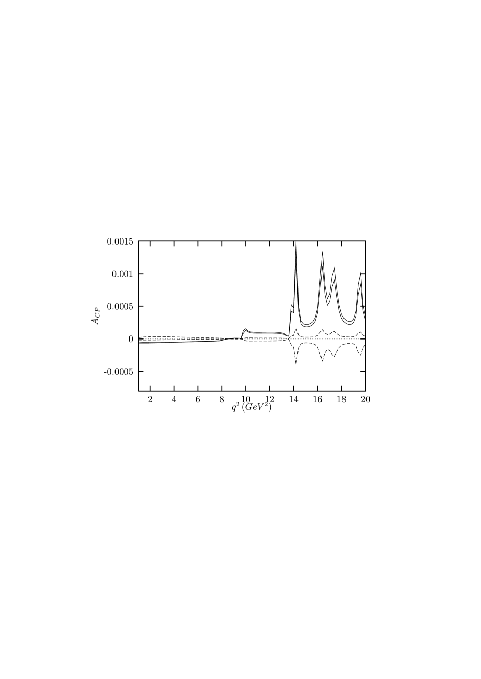
Figure 3: $A_{CP}$ as a function of $q^{2}$ for $sin\,\theta=0.1$, $\bar{\epsilon}_{N,bb}^{D}=40\,m_{b}$ in the region $|r_{tb}|<1$, at the scale $\mu=m_{b}$, including LD effects. Here $A_{CP}$ is restricted in the region bounded by solid lines for $C_{7}^{eff}>0$ and by dashed lines for $C_{7}^{eff}<0$ .

In figs. 3 (4) we plot $A_{CP}$ of the decay $B\rightarrow K^{*}l^{+}l^{-}$ with respect to the dilepton mass square, $q^{2}$, for $\bar{\epsilon}_{N,bb}^{D}=40\,m_{b}$, $sin\,\theta=0.1$ ($sin\,\theta=0.5$) in the case where the ratio $|r_{tb}|<1.$ For $C_{7}^{eff}>0$, $A_{CP}$ is restricted in the region bounded by solid lines and for $C_{7}^{eff}<0$ it lies between dashed lines. $A_{CP}$ changes sign almost at the $q^{2}$ value $q^{2}\sim 9\,GeV^{2}$ for $C_{7}^{eff}>0$ case. However, for $C_{7}^{eff}<0$, it can have both signs for any $q^{2}$ value. $A_{CP}$ enhances strongly with increasing value of $sin\,\theta$. For completeness, we present the average value of $A_{CP}$ for three different phase angles ($sin\theta=0.1,\,0,5,\,0.9$) in two different dilepton mass regions (Table 3),

$sin\theta$	$C_{7}^{eff}>0$	$C_{7}^{eff}<0$	$q^{2}$ regions
$0.1$	$-3.35\,10^{-4}\leq\bar{A}_{CP}\leq-0.74\,10^{-4}$	$-0.74\,10^{-4}\leq\bar{A}_{CP}\leq 1.71\,10^{-4}$	I
	$0.43\,10^{-4}\leq\bar{A}_{CP}\leq 3.22\,10^{-4}$	$-1.05\,10^{-4}\leq\bar{A}_{CP}\leq 0.43\,10^{-4}$	II
$0.5$	$-1.05\,10^{-2}\leq\bar{A}_{CP}\leq-1.04\,10^{-2}$	$-0.25\,10^{-2}\leq\bar{A}_{CP}\leq 0.55\,10^{-2}$	I
	$0.97\,10^{-2}\leq\bar{A}_{CP}\leq 1.17\,10^{-2}$	$-0.34\,10^{-2}\leq\bar{A}_{CP}\leq 0.14\,10^{-2}$	II
$0.9$	$-3.32\,10^{-2}\leq\bar{A}_{CP}\leq-0.91\,10^{-2}$	$-0.90\,10^{-2}\leq\bar{A}_{CP}\leq 2.72\,10^{-2}$	I
	$0.53\,10^{-2}\leq\bar{A}_{CP}\leq 2.66\,10^{-2}$	$-1.86\,10^{-2}\leq\bar{A}_{CP}\leq 0.53\,10^{-2}$	II

Table 3: The average CP asymmetry $\bar{A}_{CP}$ for regions I ( $1\,GeV\leq\sqrt{q}^{2}\leq m_{J/\psi}-20\,MeV$ ) and II ($m_{J/\psi}+20\,MeV\leq\sqrt{q}^{2}\leq m_{\psi^{\prime}}-20\,MeV$ )

Figs. 5 and 6 are devoted to $sin\,\theta$ dependence of $A_{CP}$ for $q^{2}=4\,GeV^{2}$ and $q^{2}=12\,GeV^{2}$ respectively. Here, $A_{CP}$ lies in the region bounded by solid lines for $C_{7}^{eff}>0$ or by dashed lines for $C_{7}^{eff}<0$. With decreasing $sin\,\theta$, $A_{CP}$ decreases as expected and the restriction region becomes narrower, for both $C_{7}^{eff}>0$ and $C_{7}^{eff}<0$. Further, for fixed $q^{2}$ values, the sign of $A_{CP}$ does not change with changing $\sin\,\theta$ for $C_{7}^{eff}>0$ , contrary to the case $C_{7}^{eff}<0$. This is informative in the determination of the sign of $C_{7}^{eff}$ with the experimental measurement of $A_{CP}$ at fixed $q^{2}$. Note that the similar situation exist for the general 2HDM with complex Yukawa couplings (see [17]).

Now we would like to summarize our results:

• $Br$ for the process under consideration is at the order of $10^{-6}$ for $|r_{tb}|<1$ and it is greater for $C_{7}^{eff}>0$ compared to $C_{7}^{eff}<0$. Further, it is not sensitive to $sin\,\theta$ especially for $C_{7}^{eff}<0$.

• $|A_{CP}|$ increases with increasing $sin\,\theta$. For $C_{7}^{eff}>0$, $A_{CP}$ changes sign at the $q^{2}$ value, $q^{2}\sim 9\,GeV^{2}$, however it can have any sign for $C_{7}^{eff}<0$. For the case $|r_{tb}|>>1$, $A_{CP}$ almost vanishes ($\sim 10^{-11}$) since $sin\,\theta$ should be small due to the restriction coming from the limit on neutron electric dipole moment.

• For the fixed value of $q^{2}$ and $C_{7}^{eff}>0$, $A_{CP}$ can be either negative or positive when $sin\,\theta$ varies. For $C_{7}^{eff}<0$, it can have both signs. This shows that with the measurement of $A_{CP}$ for fixed $q^{2}$, it is possible to detect the sign of $C_{7}^{eff}$, which is an interesting result.

Therefore, the experimental investigation of $A_{CP}$ ensure a crucial test for new physics and also the sign of $C_{7}^{eff}$.

Appendix

Appendix A The Wilson coefficients in the SM and the functions appear in these coefficients

The initial values of the Wilson coefficients for the relevant process in the SM are [5]

$$C^{SM}_{1,3,\dots 6,11,12}(m_{W}) = 0\,\,,$$

$$C^{SM}_{2}(m_{W}) = 1\,\,,$$

$$C_{7}^{SM}(m_{W}) = \frac{3x^{3}-2x^{2}}{4(x-1)^{4}}\ln x+\frac{-8x^{3}-5x^{2}+7x}{24(x-1)^{3}}\,\,,$$

$$C_{8}^{SM}(m_{W}) = -\frac{3x^{2}}{4(x-1)^{4}}\ln x+\frac{-x^{3}+5x^{2}+2x}{8(x-1)^{3}}\,\,,$$

$$C_{9}^{SM}(m_{W}) = -\frac{1}{sin^{2}\theta_{W}}B(x)+\frac{1-4\sin^{2}\theta_{W}}{\sin^{2}\theta_{W}}C(x)-D(x)+\frac{4}{9},\,\,,$$

$$C_{10}^{SM}(m_{W}) = \frac{1}{\sin^{2}\theta_{W}}(B(x)-C(x))\,\,,$$

and the primed ones are

$$C^{\prime SM}_{1,\dots 12}(m_{W}) = 0.$$ (47)

The functions appear in these coefficients are

$$B(x) = \frac{1}{4}\left[\frac{-x}{x-1}+\frac{x}{(x-1)^{2}}\ln x\right]\,\,,$$

$$C(x) = \frac{x}{4}\left[\frac{x/2-3}{x-1}+\frac{3x/2+1}{(x-1)^{2}}\ln x\right]\,\,,$$

$$D(x) = \frac{-19x^{3}/36+25x^{2}/36}{(x-1)^{3}}+\frac{-x^{4}/6+5x^{3}/3-3x^{2}+16x/9-4/9}{(x-1)^{4}}\ln x\,\,,$$ (48)

and in the coefficients $C_{i}^{(\prime)H}$ (eqs. (20) and (21)) are

$$F_{1}(y) = \frac{y(7-5y-8y^{2})}{72(y-1)^{3}}+\frac{y^{2}(3y-2)}{12(y-1)^{4}}\,\ln y\,\,,$$

$$F_{2}(y) = \frac{y(5y-3)}{12(y-1)^{2}}+\frac{y(-3y+2)}{6(y-1)^{3}}\,\ln y\,\,,$$

$$G_{1}(y) = \frac{y(-y^{2}+5y+2)}{24(y-1)^{3}}+\frac{-y^{2}}{4(y-1)^{4}}\,\ln y\,\,,$$

$$G_{2}(y) = \frac{y(y-3)}{4(y-1)^{2}}+\frac{y}{2(y-1)^{3}}\,\ln y\,\,,$$

$$H_{1}(y) = \frac{1-4sin^{2}\theta_{W}}{sin^{2}\theta_{W}}\,\,\frac{xy}{8}\,\left[\frac{1}{y-1}-\frac{1}{(y-1)^{2}}\ln y\right]-y\left[\frac{47y^{2}-79y+38}{108(y-1)^{3}}-\frac{3y^{3}-6y+4}{18(y-1)^{4}}\ln y\right]\,\,,$$

$$L_{1}(y) = \frac{1}{sin^{2}\theta_{W}}\,\,\frac{xy}{8}\,\left[-\frac{1}{y-1}+\frac{1}{(y-1)^{2}}\ln y\right]\,\,.$$

Appendix B 3 Higgs doublet model

We consider three complex, $SU(2)$ doublet scalar fields $\phi_{i}\,(i=1,2,3)$. The gauge and $CP$ invariant Higgs potential which spontaneously breaks $SU(2)\times U(1)$ down to $U(1)$ can be written as:

$$V(\phi_{1},\phi_{2},\phi_{3}) = c_{1}(\phi_{1}^{+}\phi_{1}-v^{2}/2)^{2}+c_{2}(\phi_{2}^{+}\phi_{2})^{2}$$ (50)

$$+ c_{3}(\phi_{3}^{+}\phi_{3})^{2}+c_{4}[(\phi_{1}^{+}\phi_{1}-v^{2}/2)+\phi_{2}^{+}\phi_{2}+\phi_{3}^{+}\phi_{3}]^{2}$$

$$+ c_{5}[(\phi_{1}^{+}\phi_{1})(\phi_{2}^{+}\phi_{2})-(\phi_{1}^{+}\phi_{2})(\phi_{2}^{+}\phi_{1})]$$

$$+ c_{6}[(\phi_{1}^{+}\phi_{1})(\phi_{3}^{+}\phi_{3})-(\phi_{1}^{+}\phi_{3})(\phi_{3}^{+}\phi_{1})]$$

$$+ c_{7}[(\phi_{2}^{+}\phi_{2})(\phi_{3}^{+}\phi_{3})-(\phi_{2}^{+}\phi_{3})(\phi_{3}^{+}\phi_{2})]$$

$$+ c_{8}[Re(\phi_{1}^{+}\phi_{2})]^{2}+c_{9}[Re(\phi_{1}^{+}\phi_{3})]^{2}+c_{10}[Re(\phi_{2}^{+}\phi_{3})]^{2}$$

$$+ c_{11}[Im(\phi_{1}^{+}\phi_{2})]^{2}+c_{12}[Im(\phi_{1}^{+}\phi_{3})]^{2}+c_{13}[Im(\phi_{2}^{+}\phi_{3})]^{2}+c_{14}$$

Here, we assume that only $\phi_{1}$ has vacuum expectation value (see section 2). The parameters $c_{i}$ are real to ensure the hermiticity of the potential term. Further, the Higgs sector does not violate $CP$ and all possible $CP$ violation effects are based on the choice of the Yukawa couplings.

The Higgs boson squared mass matrix can be obtained by the expression

$$m_{ij}=\frac{\partial^{2}V(\phi_{1}\,,\phi_{2}\,,\phi_{3})}{\partial\theta_{i}\,\partial\theta_{j}}\,\,.$$ (51)

Here $\theta_{i}$ are real fields satisfying

$$\chi^{+} = \theta_{1}+i\theta_{2}\,,$$

$$H^{+} = \theta_{3}+i\theta_{4}\,,$$

$$F^{+} = \theta_{5}+i\theta_{6}\,,$$

$$\chi^{0} = \theta_{7}\,,$$

$$H^{2} = \theta_{8}\,,$$

$$H^{4} = \theta_{9}\,,$$

$$H^{0} = \theta_{10}\,,$$

$$H^{1} = \theta_{11}\,,$$

$$H^{3} = \theta_{12}\,,$$ (52)

where $\chi^{+}$, $\chi^{0}$ and $H^{0}$ are the SM particles and $H^{+}$, $F^{+}$, $H^{i}\,(i=1,2,3,4)$ are new particles existing in 3HDM (see eq. (12) ). Note that, these fields are mass eigenstates, thanks to choice eq.(12). Diagonalizing this matrix, we get masses of new Higgs particles as:

$$m_{H\pm} = \frac{v^{2}}{2}c_{5}\,\,,$$

$$m_{F\pm} = \frac{v^{2}}{2}c_{6}\,\,,$$

$$m_{H^{1}} = \frac{v^{2}}{2}c_{8}\,\,,$$

$$m_{H^{2}} = \frac{v^{2}}{2}c_{11}\,\,,$$

$$m_{H^{3}} = \frac{v^{2}}{2}c_{9}\,\,,$$

$$m_{H^{4}} = \frac{v^{2}}{2}c_{12}\,\,.$$ (53)

In eq. (52), $\chi^{+}$ and $\chi^{0}$ are golstone bosons, which can be eaten up in unitary gauge, $H^{0}$ is the SM Higgs which has mass $m_{H^{0}}=2v^{2}(c_{1}+c_{4})$. $H^{1}$, $H^{3}$ are scalar and $H^{2}$, $H^{4}$ are pseudoscalar particles due to new physics. Note that $H^{1}$ and $H^{2}$ are denoted by $h^{0}$ and $A^{0}$ in the literature.

For completeness, we also present the kinetic term for the 3HDM:

$$(D_{\mu}\phi_{i})^{+}D^{\mu}\phi_{i}= (\partial_{\mu}\phi_{i}^{+}+i\frac{g^{\prime}}{2}B_{\mu}\phi^{+}_{i}+i\frac{g}{2}\phi^{+}_{i}\frac{\vec{\tau}}{2}\vec{W}_{\mu})$$ (54)

$$(\partial^{\mu}\phi_{i}-i\frac{g^{\prime}}{2}B^{\mu}\phi_{i}-i\frac{g}{2}\phi_{i}\frac{\vec{\tau}}{2}\vec{W}^{\mu})$$

where

$$\phi_{i}=\left(\begin{array}[]{c c}\phi^{+}\\ \phi^{0}\end{array}\right)\,\,i=1,2,3\,.$$ (57)

Appendix C The form factors for the decay $B\rightarrow K^{*}l^{+}l^{-}$

The structure functions appear in eq. (35) are

$$A = -C_{9}^{eff}\frac{V}{m_{B}+m_{K^{*}}}-4C_{7}^{eff}\frac{m_{b}}{q^{2}}T_{1}~{},$$

$$B_{1} = -C_{9}^{eff}(m_{B}+m_{K^{*}})A_{1}-4C_{7}^{eff}\frac{m_{b}}{q^{2}}(m_{B}^{2}-m_{K^{*}}^{2})T_{2}~{},$$

$$B_{2} = -C_{9}^{eff}\frac{A_{2}}{m_{B}+m_{K^{*}}}-4C_{7}^{eff}\frac{m_{b}}{q^{2}}\left(T_{2}+\frac{q^{2}}{m_{B}^{2}-m_{K^{*}}^{2}}T_{3}\right)~{},$$

$$B_{3} = -C_{9}^{eff}\frac{2m_{K^{*}}}{q^{2}}(A_{3}-A_{0})+4C_{7}\frac{m_{b}}{q^{2}}T_{3}~{},$$

$$C = -C_{10}\frac{V}{m_{B}+m_{K^{*}}}~{},$$

$$D_{1} = -C_{10}(m_{B}+m_{K^{*}})A_{1}~{},$$

$$D_{2} = -C_{10}\frac{A_{2}}{m_{B}+m_{K^{*}}}~{},$$

$$D_{3} = -C_{10}\frac{2m_{K^{*}}}{q^{2}}(A_{3}-A_{0})~{}.$$ (58)

We use the $q^{2}$ dependent expression which is calculated in the framework of light-cone QCD sum rules in [31] to calculate the hadronic formfactors $V,~{}A_{1},~{}A_{2},~{}A_{0},~{}T_{1},~{}T_{2}$ and $T_{3}$:

$$F(q^{2})=\frac{F(0)}{1-a_{F}\frac{q^{2}}{m_{B}^{2}}+b_{F}(\frac{q^{2}}{m_{B}^{2}})^{2}}\,,$$ (59)

where the values of parameters $F(0)$, $a_{F}$ and $b_{F}$ are listed in Table 4.

	$F(0)$	$a_{F}$	$b_{F}$
$A_{1}$	$0.34\pm 0.05$	$0.60$	$-0.023$
$A_{2}$	$0.28\pm 0.04$	$1.18$	$0.281$
$V$	$0.46\pm 0.07$	$1.55$	$0.575$
$T_{1}$	$0.19\pm 0.03$	$1.59$	$0.615$
$T_{2}$	$0.19\pm 0.03$	$0.49$	$-0.241$
$T_{3}$	$0.13\pm 0.02$	$1.20$	$0.098$

Table 4: The values of parameters existing in eq.(59) for the various form factors of the transition $B\rightarrow K^{*}$.

Figure 1: Differential $Br$ as a function of $q^{2}$ for $sin\,\theta=0.5$, $\bar{\epsilon}_{N,bb}^{D}=40\,m_{b}$ in the region $|r_{tb}|<1$, at the scale $\mu=m_{b}$, including LD effects. Here differential $Br$ is restricted in the region bounded by solid lines for $C_{7}^{eff}>0$ and by dashed lines for $C_{7}^{eff}<0$. Dotted line represents the SM result withouth LD effects.

Figure 2: Differential $Br$ as a function of $sin\,\theta$ for $q^{2}=12\,GeV^{2}$, $\bar{\epsilon}_{N,bb}^{D}=40\,m_{b}$ in the region $|r_{tb}|<1$, at the scale $\mu=m_{b}$, including LD effects. Here differential $Br$ is restricted in the region bounded by solid lines for $C_{7}^{eff}>0$ and by dashed lines for $C_{7}^{eff}<0$. Dotted line represents the SM result withouth LD effects.

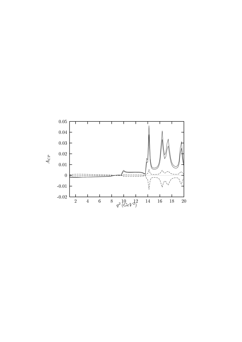
Figure 4: The same as Fig 3, but for $sin\,\theta=0.5$.

Figure 5: $A_{CP}$ as a function of $sin\,\theta$ for $q^{2}=4\,GeV^{2}$, $\bar{\epsilon}_{N,bb}^{D}=40\,m_{b}$ in the region $|r_{tb}|<1$, at the scale $\mu=m_{b}$, including LD effects. Here $A_{CP}$ is restricted in the region bounded by solid lines for $C_{7}^{eff}>0$ and by dashed lines for $C_{7}^{eff}<0$.

Figure 6: The same as Fig 5, but for $q^{2}=12\,GeV^{2}$.

References

[1] J. L. Hewett, in Proc. of the Annual SLAC Summer
Institute, ed. L. De Porcel and C. Dunwoode, SLAC-PUB-6521 (1994)
[2] W. -S. Hou, R. S. Willey and A. Soni,
Phys. Rev. Lett.58 (1987) 1608.
[3] N. G. Deshpande and J. Trampetic,
Phys. Rev. Lett.60 (1988) 2583.
[4] C. S. Lim, T. Morozumi and A. I. Sanda,
Phys. Lett.B218 (1989) 343.
[5] B. Grinstein, M. J. Savage and M. B. Wise,
Nucl. Phys.B319 (1989) 271.
[6] C. Dominguez, N. Paver and Riazuddin,
Phys. Lett.B214 (1988) 459.
[7] N. G. Deshpande, J. Trampetic and K. Ponose,
Phys. Rev.D39 (1989) 1461.
[8] P. J. O’Donnell and H. K. Tung,
Phys. Rev.D43 (1991) 2067.
[9] N. Paver and Riazuddin,
Phys. Rev.D45 (1992) 978.
[10] A. Ali, T. Mannel and T. Morozumi,
Phys. Lett.B273 (1991) 505.
[11] A. Ali, G. F. Giudice and T. Mannel,
Z. Phys.C67 (1995) 417.
[12] C. Greub, A. Ioannissian and D. Wyler,
Phys. Lett.B346 (1995) 145;
D. Liu Phys. Lett.B346 (1995) 355;
G. Burdman, Phys. Rev.D52 (1995) 6400:
Y. Okada, Y. Shimizu and M. Tanaka Phys. Lett.B405 (1997) 297.
[13] A. J. Buras and M. Münz,
Phys. Rev.D52 (1995) 186.
[14] N. G. Deshpande, X. -G. He and J. Trampetic,
Phys. Lett.B367 (1996) 362.
[15] W. Jaus and D. Wyler,
Phys. Rev.D41 (1990) 3405.
[16] T. M.Aliev, E. Iltan hep-ph/ 9804458 (1998), to appear
in Phys. Lett. B
[17] E. Iltan hep-ph/ 9902223 (1999).
[18] D. Atwood, L. Reina and A. Soni,
Phys. Rev.D53 (1996) 119.
[19] T. M.Aliev, E. Iltan hep-ph/ 9803272 (1998), to appear
in J. Phys. G. Nucl. Part.
[20] B. Grinstein, R. Springer, and M. Wise,
Nuc. Phys. B339 (1990) 269; R. Grigjanis, P.J. O’Donnel,
M. Sutherland and H. Navelet, Phys. Lett. B213 (1988) 355;
Phys. Lett. B286 (1992) E, 413;
G. Cella, G. Curci, G. Ricciardi and
A. Viceré, Phys. Lett. B325 (1994) 227,
Nucl. Phys. B431 (1994) 417.
[22] T. M. Aliev, and E. Iltan,
Phys. Rev.D58 (1998) 095014.
[23] A. I. Vainshtein, V. I. Zakharov, L. B. Okun and
M. A. Shifman,
Sov. J. Nucl. Phys.24 (1976) 427.
[24] M. Ciuchini, G. Degrassi, P. Gambino and G. I. Giudice,
Nucl. Phys.B527 (1998) 21.
[25] F. M. Borzumati and C. Greub,
Phys. Rev.D58 (1998) 0784004
[26] P. Colangelo, F. De Fazio, P. Santorelli and E. Scrimieri,
Phys. Rev.D53 (1996) 3672.
[27] T. M. Aliev, A. Özpineci and M.Savcı,
Phys. Rev.D56 (1997) 4260.
[28] M. S. Alam Collaboration, to appear in ICHEP98 Conference
(1998)
[29] T. M. Aliev, G. Hiller and E. O. Iltan,
Nucl. Phys.B515 (1998) 321.
[30] D. B. Chao, K. Cheung and W. Y. Keung,
hep-ph/ 98011235 (1998).
[31] P. Ball and V. Braun,
Phys. Rev.D57 (1998) 4260.