Precision Calculation Project Report

Abstract

The complete list of definitions for quantities relevant in the analysis of SLD/LEP-1 results around the $Z$-resonance is given. The common set of conventions adopted by the programs TOPAZ0 and ZFITTER, following the recommendations of the LEP electroweak working group, is reviewed. The relevance of precision calculations is discussed in detail both for pseudo-observables (PO) and for realistic observables (RO). The model-independent approach is also discussed. A critical assessment is given of the comparison between TOPAZ0 and ZFITTER.

1 Motivations for the Upgrading of Precision Calculations

The main motivation for upgrading precision calculations around the $Z$-resonance with the programs TOPAZ0 [1] and ZFITTER [2] and for making public the results is a reflection of questions frequently asked by the experimental community:

A complete definition of lineshape and asymmetry pseudo observables (POs), together with the residual Standard Model (SM) dependence in model-independent fits, is needed. This includes a description on what is actually taken from the SM.

Both codes calculate POs. A definition of these POs is needed, showing that TOPAZ0 [1] and ZFITTER [2] use the same definition so that any discrepancy is really a measure of missing higher-order corrections. This should include quantities like $M_{{}_{Z}}$, $\Gamma_{{}_{Z}}$, $\Gamma_{f}$, $\sigma^{0}_{{h}}$ and $A^{0}_{{}_{\rm FB}}$, and also $g^{f}_{{}_{V}}$, $g^{f}_{{}_{A}}$ and $\sin^{2}\theta^{\rm lept}_{\rm{eff}}$.

1.1 Goals of this Report

In 1989 the CERN Report ‘$Z$ Physics at LEP1’, [3] has provided a central documentation of the theoretical basis for the physics analysis of the LEP results. Although being quite comprehensive, an update on the discussion of radiative corrections became necessary in 1995, detailed in the CERN report ‘Reports of the Working Group on Precision Calculations for the $Z$ Resonance’, [4]. The structure of the latter report was determined by a central part describing the situation for the electroweak observables as obtained by various independent calculations, including the remaining theoretical uncertainties, followed by comprehensive descriptions of the QCD aspects of electroweak $Z$ physics.

A new step was taken in early 1998 with a note on the ‘Upgrading of Precision Calculations for Electroweak Observables’ [5], where one focused on the calculation of the pseudo-observables.

It is now time to move a step forward and fully revise the comparisons not only for POs but also for realistic observables (ROs), i.e., total cross-sections and forward-backward asymmetries, both extrapolated and with realistic cuts. Our goal, therefore, has been to upgrade and to compare critically the complete TOPAZ0 and ZFITTER predictions with a particular emphasis on demanding the following criteria:

• Comparisons, after the upgrading, should be consistently better than what they were in earlier studies.

• At the peak all relative deviations among total cross-sections and absolute deviations among asymmetries should be below $0.1$ per-mill.

• At the wings, typically $\sqrt{s}=M_{{}_{Z}}\pm 1.8\,\;\mathrm{GeV}$, they should be below $0.3$ per-mill.

It is important to observe that a comparison for ROs at the level of $10^{-4}$ has never been attempted before.

The numerical results reported in this article are calculated with TOPAZ0 version 4.4 [6] and ZFITTER version 5.20 [7]. After a careful examination of the new upgrading of TOPAZ0 and ZFITTER contained in these versions we are able to report in general a good agreement in our comparisons. The worst case for pseudo-observables is represented by the $b\overline{b}$-channel. This fact, however, was largely expected: this particular channel is where the next-to-leading two-loop electroweak corrections are missing and, therefore, here is where we face a larger level of theoretical uncertainties. We find satisfactory agreement in all the comparisons performed for realistic observables but one: the inclusion of initial-final QED interference in the presence of realistic cuts, i.e., acollinearity and polar angle cuts and energy thresholds. This fact will be discussed in detail in Section 7.

In this context we would like to emphasise that the implementation of the next-to-leading corrections, as well as of any higher-order corrections, makes stable all theoretical predictions: the degree of arbitrariness of the various implementations is reduced with the introduction of newly computed terms.

Coming back to the reason for the present upgrading, we may say that there are additional motivations for it, which we illustrate in the following section.

1.2 List of Improved I/O Parameters

For all results, if not stated otherwise we use

$$M_{{}_{Z}}=91.1867\,\;\mathrm{GeV}.$$ (1)

In fixing the set of input parameters we take the lepton masses as in PDG’98 [8]. They are as follows:

$$m_{e}=0.51099907\,\;\mathrm{MeV},\quad m_{\mu}=105.658389\,\;\mathrm{MeV},\quad m_{\tau}=1.77705\,\;\mathrm{GeV}.$$ (2)

Since all renormalization schemes use the Fermi constant, $G_{{\scriptscriptstyle{F}}}$, we refer to a recent calculation [9], giving an improved value of $G_{{\scriptscriptstyle{F}}}=1.16637(1)\times 10^{-5}\,\;\mathrm{GeV}^{-2}$ to be compared with the old one, $G_{{\scriptscriptstyle{F}}}=1.16639(2)\times 10^{-5}\,\;\mathrm{GeV}^{-2}$ [8].

An important issue concerns the evaluation of $\alpha_{\rm QED}$ at the mass of the $Z$. There is an agreement in our community on using the following strategy. Define

$$\alpha(M_{{}_{Z}})=\frac{\alpha(0)}{1-\Delta\alpha^{(5)}(M_{{}_{Z}})-\Delta_{\rm{top}}(M_{{}_{Z}})-\Delta^{\alpha\alpha_{{}_{S}}}_{\rm{top}}(M_{{}_{Z}})}\;,$$ (3)

where one has $\Delta\alpha^{(5)}(M_{{}_{Z}})=\Delta\alpha_{\rm{lept}}+\Delta\alpha^{(5)}_{\rm{had}}$. In both codes the input parameter is now $\Delta\alpha^{(5)}_{\rm{had}}$, as it is the contribution with the largest uncertainty, while the calculation of the top contributions to $\Delta\alpha$ is left for the code. This should become common to all codes.

The programs TOPAZ0 and ZFITTER include the recently computed ${\mathcal{O}}\left(\alpha^{3}\right)$ terms of [10] for $\Delta\alpha_{\rm{lept}}$, and use as default $\Delta\alpha^{(5)}_{\rm{had}}=0.0280398$ taken from [11]. As explained above the latter parameter can be reset by the user. Using the default one obtains $1/\alpha^{(5)}(M_{{}_{Z}})=128.877$, to which one must add the $t\overline{t}$ contribution and the ${\mathcal{O}}\left(\alpha\alpha_{{}_{S}}\right)$ correction induced by the $t\overline{t}$ loop with gluon exchange [12].

For the improved calculation of $\Delta\alpha_{\rm{lept}}$ we find the result as reported in Tab.(1). For the $t$ contribution we derive the results listed in Tab.(2). For the ${\mathcal{O}}\left(\alpha\alpha_{{}_{S}}\right)$ corrections induced by the $t\overline{t}$ loop we report the results in Tab.(3) with the value of $\alpha_{{}_{S}}(m_{t})$ as reported in Tab.(4).

	$10^{4}\times\Delta\alpha_{\rm{lept}}$
TOPAZ0	314.97644
ZFITTER	314.97637

Table 1: $10^{4}\times\Delta_{\rm{lept}}(M_{{}_{Z}})$.

$m_{t}\,$[GeV]	168.8	173.8	178.8
TOPAZ0	-0.622230	-0.585844	-0.552589
ZFITTER	-0.622230	-0.585844	-0.552589

Table 2: $10^{4}\times\Delta_{\rm top}(M_{{}_{Z}})$.

$\alpha_{{}_{S}}(M_{{}_{Z}})/m_{t}\,$[GeV]	168.8	173.8	178.8
0.116	-0.108440	-0.101593	-0.095371
	-0.108440	-0.101593	-0.095371
0.119	-0.110994	-0.103976	-0.097599
	-0.110994	-0.103962	-0.097600
0.122	-0.113536	-0.106347	-0.099816
	-0.113536	-0.106347	-0.099816

Table 3: TOPAZ0 (first row) / ZFITTER (second row) results for $10^{4}\times\Delta^{\alpha\alpha_{{}_{S}}}_{\rm{top}}(M_{{}_{Z}})$.

$\alpha_{{}_{S}}(M_{{}_{Z}})/m_{t}\,$[GeV]	168.8	173.8	178.8
0.116	0.10631	0.10589	0.10548
	0.10631	0.10589	0.10548
0.119	0.10881	0.10837	0.10795
	0.10881	0.10837	0.10795
0.122	0.11130	0.11084	0.11040
	0.11130	0.11084	0.11040

Table 4: TOPAZ0 (first row) / ZFITTER (second row) results for $\alpha_{{}_{S}}(m_{t})$.

2 Analysis of the Measurements

In the following we take the LEP-1 measurements of hadronic and leptonic cross sections and leptonic forward-backward asymmetries as an example to discuss the data analysis strategy.

2.1 The Experimental Strategy

Technically, each LEP experiment extracts POs, namely $M_{{}_{Z}},\Gamma_{{}_{Z}},\sigma^{0}_{{h}},R_{e,\mu,\tau}$ and $A^{0,e,\mu,\tau}_{{}_{\rm FB}}$ (see Section 3.1 for a definition), from their measured cross-sections and asymmetries (realistic observables). The four sets of POs are combined, taking correlated errors between the LEP experiments into account, in order to obtain a LEP-average set of POs [13]. The latter is then interpreted, for example within the frame-work of the Minimal Standard Model.

Ideally, one would like to combine the results of the LEP experiments at the level of the measured cross-sections and asymmetries - a goal that has never been achieved so far because of the intrinsic complexity, given the large number of measurements with different cuts and the complicated structure of the experimental covariance matrices relating their errors. As a consequence, the practical attitude of the four LEP experiments is to stay with a Model-Independent (MI) fit, i.e., from ROs $\to$ POs ($\,\oplus\,$ a Standard Model remnant) for each experiment, and to average the four sets of POs. The result of this procedure is a set of best values for POs which are of course important quantities in their own right. The extraction of Lagrangian parameters, $M_{{}_{Z}},m_{t},M_{{}_{H}}$, $\alpha_{{}_{S}}(M^{2}_{{}_{Z}})$ and $\alpha(M^{2}_{{}_{Z}})$, is based on the LEP-averaged POs.

There remain several questions to be answered: the main one is, to what extend are the POs a Model-Independent (MI) description of the measurements? Furthermore, are they valid even in the case where the Standard Model is not the correct theory? Note, that many effects are absorbed into the POs. Since POs are determined by fitting realistic observables (ROs), one has to clarify what is actually taken from the SM (such as imaginary parts and parts which have been moved to $Z-\gamma$ interference terms and photon-exchange terms) making the MI results dependent on the SM.

The POs are unsatisfactory for many reasons but to some level of accuracy they describe well the experimental measurements at the $Z$ peak. How well and what is lost in the reduction ROs $\to$ POs is exactly the kind of question that the LEP community is trying to answer.

In the case of the Standard Model and the measurements of hadronic and leptonic cross sections and leptonic forward-backward asymmetries at LEP-1, it has been tested by each LEP experiment how the results on the SM parameters differ between a SM fit to its own measured ROs, and a SM fit to the POs which themselves are derived in an MI fit to the same ROs [14]. In the MI fit to determine the POs, the SM initialisation has been performed with $M_{{}_{Z}}=91.1867\,$GeV, $m_{t}=175\,$GeV, $M_{{}_{H}}=150\,$GeV, $\alpha_{{}_{S}}(M^{2}_{{}_{Z}})=0.119$, and $\Delta\alpha^{(5)}_{\rm{had}}(M^{2}_{{}_{Z}})=0.02804$ ($1/\alpha^{(5)}(M^{2}_{{}_{Z}})=128.878$). In the two SM fits (to ROs and to POs) to be compared, in both cases $m_{t}=173.8\pm 5.0\,$GeV and $\Delta\alpha^{(5)}_{\rm{had}}(M^{2}_{{}_{Z}})=0.02804\pm 0.00065$ ($1/\alpha^{(5)}(M^{2}_{{}_{Z}})=128.878\pm 0.090$) are included as external constraints.

For each experiment, the largest difference in central values, relative to the fitted errors, is observed for the value of the SM parameter $M_{{}_{Z}}$, up to 30% of the fit error. The fit error itself is unchanged. The shift in central value also depends on the Higgs mass used in the SM initialisation of the MI fit to determine the POs. One reason for these observations is the following, but more detailed studies are needed. The experimentally preferred value of the Higgs-boson mass may be different from the value of the Higgs-boson mass used in the SM initialisation of the MI fit. In particular, the latter affects the value of the $Z-\gamma$ interference term for the hadronic cross-section which must be taken from the SM for the MI fit. Since the $Z-\gamma$ interference term for the hadronic cross-section is highly anti-correlated with $M_{{}_{Z}}$ when derived from the LEP-1 data, the choice of $M_{{}_{H}}$ affects the fitted value of $M_{{}_{Z}}$ in the MI fit, and subsequently the extraction of SM parameters. For the other four SM parameters, the observed differences in fitted central values and errors are usually below 10% to 15% of the fit error on this parameter.

As the LEP average is a factor of two more precise, care has to be taken in the averaging procedure. An alternative way to extract SM parameters from the LEP measurements, avoiding the intermediate step of POs, is to average directly the SM parameters which have been obtained by each experiment through a SM fit to its own ROs. This alternative should indeed also be pursued by the experiments.

2.2 The Theoretical Strategy

Within the context of the SM the ROs are described in terms of some set of amplitudes

$$A_{{}_{\rm SM}}=A_{\gamma}+A_{{}_{Z}}+\mbox{non-factorizable},$$ (4)

where the last term is due to all those contributions that do not factorize into the Born-like amplitude, e.g., weak boxes. Once the matrix element $A_{{}_{\rm SM}}$ is computed, squared and integrated to obtain the cross section, a convolution with initial- and final-state QED and final-state QCD radiation follows:

$$\sigma(s)=\int dz~{}H_{\rm in}(z,s)\,H_{\rm fin}(z,s)\,{\hat{\sigma}}(zs),$$ (5)

where $H_{\rm in}(z,s)$ and $H_{\rm fin}(z,s)$ are so-called, radiator or flux functions accounting for Initial- (Final-) State Radiation, ISR (FSR), respectively, and ${\hat{\sigma}}(zs)$ is the kernel cross-section of the hard process, evaluated at the reduced squared centre-of-mass energy $s^{\prime}=zs$.

It is a well-known fact that the structure of the matrix element changes after inclusion of higher-order electroweak corrections. One needs the introduction of complex-valued form-factors which depend on the two Mandelstam variables $s$ and $t$. The separation into insertions for the $\gamma$ exchange and for the $Z$ exchange is lost.

The weak boxes are present as non-resonating insertions to the electroweak form-factors. At the $Z$ resonance, the one-loop weak box terms are small, with relative contributions $\leq 10^{-4}$. If we neglect them, the $t$-dependence is turned off. The $t$-dependence would also spoil factorisation of the form-factors into products of effective vector and axial-vector couplings. In all comparisons of ROs presented in this report, the weak boxes are taken into account because we go off resonance up to $\sqrt{s}=M_{{}_{Z}}\pm 3$ GeV.

Full factorisation is re-established by neglecting various terms that are of the order ${\mathcal{O}}\left(\alpha{\Gamma_{{}_{Z}}}/{M_{{}_{Z}}}\right)$. The resulting effective vector and axial-vector couplings are complex valued and dependent on $s$. The factorisation is the result of a variety of approximations which are valid at the $Z$ resonance to the accuracy needed, and which are indispensable in order to relate POs to ROs.

After the above mentioned series of approximations we arrive at the so called $Z$-boson pole approximation, which is actually equivalent to setting $s=M^{2}_{{}_{Z}}$ in the form-factors. After de-convoluting ROs of QED and QCD radiation the set of approximations transform ROs into POs.

A source of potential ambiguity is linked to the adopted strategy for extracting MI POs from the measured ROs. Indeed, the full SM calculation in a MI analysis is performed only once at the beginning where one needs to specify in addition to $M_{{}_{Z}}$, which is also a PO, the (remaining) relevant SM parameters $m_{t},M_{{}_{H}},\alpha(M_{{}_{Z}}),\alpha_{{}_{S}}(M_{{}_{Z}})$ for the SM-complement of the MI parameterisation, ${\rm RO}={\rm RO}({\rm PO}\oplus{\overline{\rm SM}})$. Subsequent steps in the MI calculation then go directly via $M_{{}_{Z}}$, total and partial widths, and $Zf\overline{f}$ couplings.

This part of the procedure is particularly cumbersome. However, one has to live with the fact that – for practical reasons – the POs will be combined among the LEP experiments and survive forever. The cross-section and asymmetry measurements will be published by the experiments, but most likely no one will ever undertake the effort to combine them. Therefore one is left with the task of making sure that the adopted procedure is acceptable.

3 Pseudo-Observables

There remains to be investigated the systematic errors arising from theory and possible ambiguities in the definition of the MI fit parameters, the POs.

3.1 Definition of Pseudo-Observables

Independent of the particular realization of the effective couplings they are complex-valued functions, due to the imaginary parts of the diagrams. In the past this fact had some relevance only for realistic observables while for pseudo-observables they were conventionally defined to include only real parts. This convention has changed lately with the introduction of next-to-leading corrections: imaginary parts, although not next-to-leading in a strict sense, are sizeable two-loop effects. These are enhanced by factors $\pi^{2}$ and sometimes also by a factor $N_{f}$, with $N_{f}$ being the total number of fermions (flavour$\,\otimes\,$colour) in the SM. Once we include the best of the two-loop terms then imaginary parts should also come in. The latest versions of TOPAZ0 and ZFITTER therefore include imaginary parts of the $Z$-resonance form factors.

The explicit formulae for the $Zf\overline{f}$ vertex are always written starting from a Born-like form of a pre-factor $\times$ fermionic current, where the Born parameters are promoted to effective, scale-dependent parameters,

$$\rho^{f}_{{}_{Z}}\gamma_{\mu}\,\left[\left(I^{(3)}_{f}+i\,a_{{\scriptscriptstyle{L}}}\right)\gamma_{+}-2\,Q_{f}\kappa^{f}_{{}_{Z}}s^{2}+i\,a_{{\scriptscriptstyle{Q}}}\right]=\gamma_{\mu}\,\bigl{(}{\mathcal{G}}^{f}_{{}_{V}}+{\mathcal{G}}^{f}_{{}_{A}}\,\gamma_{5}\bigr{)},$$ (6)

where $\gamma_{+}=1+\gamma_{5}$ and $a_{{\scriptscriptstyle{Q}},{\scriptscriptstyle{L}}}$ are the SM imaginary parts. Note that imaginary parts are always factorized in ZFITTER and added linearly in TOPAZ0.

By definition, the total and partial widths of the $Z$ boson include all corrections, also QED and QCD corrections. The partial decay width is therefore described by the following expression:

$$\Gamma_{f}\equiv\Gamma\left(Z\to f\overline{f}\right)=4\,c_{f}\,\Gamma_{0}\,\bigl{(}|{\mathcal{G}}^{f}_{{}_{V}}|^{2}\,R^{f}_{{\scriptscriptstyle{V}}}+|{\mathcal{G}}^{f}_{{}_{A}}|^{2}\,R^{f}_{{\scriptscriptstyle{A}}}\bigr{)}+\Delta_{{}_{\rm EW/QCD}}\;,$$ (7)

where $c_{f}=1$ or $3$ for leptons or quarks $(f=l,q)$, and the radiator factors $R^{f}_{{\scriptscriptstyle{V}}}$ and $R^{f}_{{\scriptscriptstyle{A}}}$ describe the final state QED and QCD corrections and take into account the fermion mass $m_{f}$.

There is a large body of contributions to the radiator factors in particular for the decay $Z\to q\overline{q}$; both TOPAZ0 and ZFITTER implement the results that have been either derived or, in few cases, confirmed in some more general setting by the Karlsruhe group, see for instance [15]. The splitting between radiators and effective couplings follows well defined recipes that can be found and referred to in [4, 16]. In particular our choice has been that top-mass dependent QCD corrections are to be considered as QCD corrections and included in the radiators and not in the effective quark couplings.

The last term,

$$\Delta_{{}_{\rm EW/QCD}}=\Gamma^{(2)}_{{}_{\rm EW/QCD}}-\frac{\alpha_{{}_{S}}}{\pi}\,\Gamma^{(1)}_{{}_{\rm EW}}\;,$$ (8)

accounts for the non-factorizable corrections. The standard partial width, $\Gamma_{0}$, is

$$\Gamma_{0}={{G_{{\scriptscriptstyle{F}}}M^{3}_{{}_{Z}}}\over{24\sqrt{2}\,\pi}}=82.945(7)\,\;\mathrm{MeV}.$$ (9)

The hadronic and leptonic pole cross-sections are defined by

$$\sigma^{0}_{{h}}=12\pi\,\frac{\Gamma_{e}\Gamma_{{}_{h}}}{M^{2}_{{}_{Z}}\Gamma^{2}_{{}_{Z}}}\qquad\sigma^{0}_{\ell}=12\pi\,\frac{\Gamma_{e}\Gamma_{l}}{M^{2}_{{}_{Z}}\Gamma^{2}_{{}_{Z}}}\;,$$ (10)

where $\Gamma_{{}_{Z}}$ is the total decay width of the $Z$ boson, i.e, the sum of all partial decay widths. Note that the mass and total width of the $Z$ boson are defined based on a propagator term $\chi$ with an $s$-dependent width:

$$\chi^{-1}(s)=s-M^{2}_{{}_{Z}}+is\Gamma_{{}_{Z}}/M_{{}_{Z}}\;.$$ (11)

The effective electroweak mixing angles (effective sinuses) are always defined by

$$4\,|Q_{f}|\sin^{2}\theta^{f}_{\rm{eff}}=1-\frac{{\rm{Re}}\;{\mathcal{G}}^{f}_{{}_{V}}}{{\rm{Re}}\;{\mathcal{G}}^{f}_{{}_{A}}}=1-\frac{g^{f}_{{}_{V}}}{g^{f}_{{}_{A}}}\;,$$ (12)

where we define

$$g^{f}_{{}_{V}}={\rm{Re}}\;{\mathcal{G}}^{f}_{{}_{V}},\qquad g^{f}_{{}_{A}}={\rm{Re}}\;{\mathcal{G}}^{f}_{{}_{A}}.$$ (13)

The forward-backward asymmetry $A_{{}_{\rm FB}}$ is defined via

$$A_{{}_{\rm FB}}=\frac{\sigma_{{}_{\rm{F}}}-\sigma_{{}_{\rm{B}}}}{\sigma_{{}_{\rm{F}}}+\sigma_{{}_{\rm{B}}}}\;,\qquad\sigma_{{}_{\rm{T}}}=\sigma_{{}_{\rm{F}}}+\sigma_{{}_{\rm{B}}}\;,$$ (14)

where $\sigma_{{}_{\rm{F}}}$ and $\sigma_{{}_{\rm{B}}}$ are the cross sections for forward and backward scattering, respectively. Before analysing the forward-backward asymmetries we have to describe the inclusion of imaginary parts. $A_{{}_{\rm FB}}$ is calculated as

$$A_{{}_{\rm FB}}=\frac{3}{4}\frac{\sigma_{{}_{\rm VA}}}{\sigma_{{}_{\rm T}}}\;,$$ (15)

where

$$\sigma_{{}_{\rm VA}} = \frac{G_{{\scriptscriptstyle{F}}}M^{2}_{{}_{Z}}}{\sqrt{2}}\,\sqrt{\rho_{e}\rho_{f}}\,Q_{e}Q_{f}{\rm{Re}}\Bigl{[}\alpha^{*}(M^{2}_{{}_{Z}}){\mathcal{G}}^{e}_{{}_{V}}{\mathcal{G}}^{f}_{{}_{A}}\chi(s)\Bigr{]}$$ (16)

$$+\frac{G_{{\scriptscriptstyle{F}}}^{2}M^{4}_{{}_{Z}}}{8\,\pi}\,\rho_{e}\rho_{f}{\rm{Re}}\Bigl{[}{\mathcal{G}}^{e}_{{}_{V}}\left({\mathcal{G}}^{e}_{{}_{A}}\right)^{*}\Bigr{]}{\rm{Re}}\Bigl{[}{\mathcal{G}}^{f}_{{}_{V}}\left({\mathcal{G}}^{f}_{{}_{A}}\right)^{*}\Bigr{]}s\,|\chi(s)|^{2}.$$

In case of quark-pair production, an additional radiator factor multiplies $\sigma_{{}_{\rm VA}}$, see also Eq.(53).

This result is valid in the realization where $\rho_{f}$ is a real quantity, i.e., the imaginary parts are not re-summed in $\rho_{f}$. In this case

$${\mathcal{G}}^{f}_{{}_{V}}={\rm{Re}}\left({\mathcal{G}}^{f}_{{}_{V}}\right)+i\,{\rm{Im}}\left({\mathcal{G}}^{f}_{{}_{V}}\right)=g^{f}_{{}_{V}}+i\,{\rm{Im}}\left({\mathcal{G}}^{f}_{{}_{V}}\right),\qquad{\mathcal{G}}^{f}_{{}_{A}}=I^{(3)}_{f}+i\,{\rm{Im}}\left({\mathcal{G}}^{f}_{{}_{A}}\right).$$ (17)

Otherwise ${\mathcal{G}}^{f}_{{}_{A}}=I^{(3)}_{f}$ is a real quantity but $\rho_{f}$ is complex valued and Eq.(16) has to be changed accordingly, i.e., we introduce

$$g^{f}_{{}_{V}}=\sqrt{\rho_{f}}\,v_{f}\;,\qquad g^{f}_{{}_{A}}=\sqrt{\rho_{f}}\,I^{(3)}_{f}\;,$$ (18)

with

$$v_{f}=I^{(3)}_{f}-2Q_{f}\sin^{2}\theta^{f}_{\rm{eff}}\;.$$ (19)

For the peak asymmetry, the presence of $\rho$’s is irrelevant since they will cancel in the ratio. We have

$$\hat{A}^{{{0}}\rm f}_{{}_{\rm FB}} = \frac{3}{4}\,\hat{A}_{e}\,\hat{A}_{f},$$

$$\hat{A}_{f} = \frac{2\,{\rm{Re}}\bigl{[}{\mathcal{G}}^{f}_{{}_{V}}\left({\mathcal{G}}^{f}_{{}_{A}}\right)^{*}\bigr{]}}{\bigl{(}\big{|}{\mathcal{G}}^{f}_{{}_{V}}\big{|}^{2}+\big{|}{\mathcal{G}}^{f}_{{}_{A}}\big{|}^{2}\bigr{)}}\;.$$ (20)

The question is what to do with imaginary parts in Eq.(20). For partial widths, as they absorb all corrections, the convention is to use

$$\big{|}{\mathcal{G}}^{f}_{{}_{V,A}}\big{|}^{2}=\bigl{(}{\rm{Re}}{\mathcal{G}}^{f}_{{}_{V,A}}\bigr{)}^{2}+\bigl{(}{\rm{Im}}{\mathcal{G}}^{f}_{{}_{V,A}}\bigr{)}^{2}.$$ (21)

On the contrary, the PO peak asymmetry $A^{0\rm f}_{{}_{\rm FB}}$ will be defined by an analogy of equation Eq.(20) where conventionally imaginary parts are not included

$$A^{0\rm f}_{{}_{\rm FB}} = \frac{3}{4}\,{\mathcal{A}}_{e}\,{\mathcal{A}}_{f},$$

$${\mathcal{A}}_{f} = \frac{2\bigl{(}g^{f}_{{}_{V}}g^{f}_{{}_{A}}\bigr{)}}{\bigl{(}g^{f}_{{}_{V}}\bigr{)}^{2}+\bigr{(}g^{f}_{{}_{A}}\bigr{)}^{2}}\;.$$ (22)

We note, that Eq.(22) is not an approximation of Eq.(20). Both are POs and both could be used as the definition. Numerically, they give very similar results: ZFITTER calculates for the two definitions in Eq.(20) and Eq.(22), $\hat{A}^{0\rm l}_{{}_{\rm FB}}=0.0160692$ and $A^{0\rm l}_{{}_{\rm FB}}=0.0160739$. The absolute difference, $0.0000047$, is more than two orders of magnitude smaller than the current experimental error of $0.00096$ [13].

In contrast to POs, which are defined, it is impossible to avoid imaginary parts for ROs without spoiling the comparison between the theoretical prediction and the experimental measurement. Then one has to start with Eq.(16). We will develop Eq.(16) in the realization where imaginary parts are added linearly. For the $ZZ$ part of the VA cross-section one derives:

$${\rm{Re}}\Bigl{[}{\mathcal{G}}^{e}_{{}_{V}}\left({\mathcal{G}}^{e}_{{}_{A}}\right)^{*}\Bigr{]}{\rm{Re}}\Bigl{[}{\mathcal{G}}^{f}_{{}_{V}}\left({\mathcal{G}}^{f}_{{}_{A}}\right)^{*}\Bigr{]}.$$ (23)

This collapses to a familiar expression if the axial-vector coefficients are real, however one cannot factorize and simplify the $\rho$’s especially away from the pole because of the $Z\gamma$ component. For the $Z\gamma$ part of the $VA$ cross-section one has the following result:

$${\rm{Re}}\bigl{[}\alpha^{*}(s)\chi(s)\bigr{]}\,{\rm{Re}}\left({\mathcal{G}}^{e}_{{}_{A}}{\mathcal{G}}^{f}_{{}_{A}}\right)-{\rm{Im}}\bigl{[}\alpha^{*}(s)\chi(s)\bigr{]}\,{\rm{Im}}\left({\mathcal{G}}^{e}_{{}_{A}}{\mathcal{G}}^{f}_{{}_{A}}\right).$$ (24)

A definition of the PO heavy quark forward-backward asymmetry parameter which would include mass effects is

$${\mathcal{A}}_{b}={{2\,g^{b}_{{}_{V}}g^{b}_{{}_{A}}}\over{\frac{1}{2}\,\left(3-\beta^{2}\right)(g^{b}_{{}_{V}})^{2}+\beta^{2}\,(g^{b}_{{}_{A}})^{2}}}\,\beta,$$ (25)

where $\beta$ is the $b$-quark velocity. For $A^{0\rm b}_{{}_{\rm FB}}$ TOPAZ0/ZFITTER find (with $m_{b}=4.7$ GeV)

$$0.102611/0.102634\quad \quad m_{b}\neq 0,$$ for

$$0.102594/0.102617\quad \quad m_{b}=0,$$ for (26)

with a $0.000017/0.000017$ difference to be compared with the experimental error of $0.0021$ [13]. The difference is very small, due to an accidental cancellation of the mass corrections between the numerator and denominator of Eq.(25). This occurs for down-type quarks where $(g^{b}_{{}_{V}})^{2}\approx(g^{b}_{{}_{A}})^{2}/2$ and where

$$A^{0\rm b}_{{}_{\rm FB}} \approx \frac{3}{4}\,\frac{2\,g^{e}_{{}_{V}}g^{e}_{{}_{A}}}{(g^{e}_{{}_{V}})^{2}+(g^{e}_{{}_{A}})^{2}}\,\frac{2\,g^{b}_{{}_{V}}g^{b}_{{}_{A}}}{(g^{b}_{{}_{V}})^{2}+(g^{b}_{{}_{A}})^{2}}\,\left(1+\delta_{\rm mass}\right),$$

$$\delta_{\rm mass} \approx 4\,\frac{m^{2}_{q}}{s}{{(g^{b}_{{}_{A}})^{2}/2-(g^{b}_{{}_{V}})^{2}}\over{(g^{b}_{{}_{V}})^{2}+(g^{b}_{{}_{A}})^{2}}}.$$ (27)

For the $c$-quark this difference is even bigger ($\sim 0.000025$ for $m_{c}=1.5$ GeV, to be compared with the experimental error of 0.0044 [13]), one more example that for $b$-quarks we meet an accidental cancellation. Note that the mass effect should be even smaller since running quark masses seem to be the relevant quantities instead of the pole ones. Therefore, our definition of the POs forward–backward asymmetry and coupling parameter will be as in Eq.(22).

The most important upgradings in the SM calculation of POs have been already described in [5]. In particular they consist of the inclusion of higher-order QCD corrections, mixed electroweak-QCD corrections [17], and next-to-leading two-loop corrections of ${\mathcal{O}}\left(\alpha^{2}m^{2}_{t}\right)$ [18].

In Ref. [18] the two-loop ${\mathcal{O}}\left(\alpha^{2}m^{2}_{t}\right)$ corrections are incorporated in the theoretical calculation of $M_{{}_{W}}$ and $\sin^{2}\theta^{\rm{lept}}_{\rm{eff}}$. More recently the complete calculation of the decay rate of the $Z$ has been made available to us [19]. The only case that is not covered is the one of final $b$-quarks, because it involves non-universal ${\mathcal{O}}\left(\alpha^{2}m^{2}_{t}\right)$ vertex corrections.

Another development in the computation of radiative corrections to the hadronic decay of the $Z$ is contained in two papers, which together provide complete corrections of ${\mathcal{O}}\left(\alpha\alpha_{{}_{S}}\right)$ to $\Gamma(Z\to q\overline{q})$ with $q=u,d,s,c$ and $b$. In the first reference of [17] the decay into light quarks is treated. In the second one the remaining diagrams contributing to the decay into bottom quarks are considered and thus the mixed two-loop corrections are complete.

3.2 Model Independent Calculations

To summarise the MI ansatz, one starts with the SM, which introduces complex-valued couplings, calculated to some order in perturbation theory. Next we define $g^{f}_{{}_{V}},g^{f}_{{}_{A}}$ as the real parts of the effective couplings and $\Gamma_{f}$ as the physical partial width absorbing all radiative corrections including the imaginary parts of the couplings and fermion mass effects. Furthermore, we introduce the ratios of partial widths

$$R_{q}=\frac{\Gamma_{q}}{\Gamma_{{}_{h}}}\;,\qquad R_{l}=\frac{\Gamma_{{}_{h}}}{\Gamma_{l}}\;,$$ (28)

for quarks and leptons, respectively.

The LEP collaborations report POs for the following sets:

$$\bigl{(}M_{{}_{Z}},\Gamma_{{}_{Z}},\sigma^{0}_{{h}},R_{f},A^{0,f}_{{}_{\rm FB}}\bigr{)};\quad\bigl{(}M_{{}_{Z}},\Gamma_{{}_{Z}},\Gamma_{{}_{h}},g^{f}_{{}_{V}},g^{f}_{{}_{A}}\bigr{)};\quad\bigl{(}M_{{}_{Z}},\Gamma_{{}_{Z}},\Gamma_{{}_{h}},\sin^{2}\theta^{f}_{\rm{eff}},\rho_{f}\bigr{)}.$$ (29)

In order to extract $g^{f}_{{}_{V}},g^{f}_{{}_{A}}$ from $\Gamma_{f}$ one has to get the SM-remnant from Eq.(7), all else is trivial. However, the parameter transformation cannot be completely MI, due to the residual SM dependence appearing inside Eq.(7).

In conclusion, the flow of the MI calculation requested by the experimental collaborations is:

1. Pick the Lagrangian parameters $m_{t},M_{{}_{H}}$ etc. for the explicit calculation of the residual SM-dependent part.

2. Perform the SM initialisation of everything, such as imaginary parts etc. giving, among other things, the complement ${\overline{\rm SM}}$.

3. Select $g^{f}_{{}_{V}},g^{f}_{{}_{A}}$.

4. Perform a SM-like calculation of $\Gamma_{f}$, but using arbitrary values for $g^{f}_{{}_{V}},g^{f}_{{}_{A}}$, and only the rest, namely

   $$R^{f}_{{\scriptscriptstyle{V}}},\quad R^{f}_{{\scriptscriptstyle{A}}}\;,\qquad\Delta_{{}_{\rm EW/QCD}}\;,\qquad{\rm{Im}}\;{\mathcal{G}}^{f}_{{}_{V}},\quad{\rm{Im}}\;{\mathcal{G}}^{f}_{{}_{A}}\;,$$ (30)

   from the SM.

An example of the parameter transformations is the following: starting from $M_{{}_{Z}},\Gamma_{{}_{Z}},\sigma^{0}_{{h}},R_{e,\mu,\tau}$ and $A^{0,e,\mu,\tau}_{{}_{\rm FB}}$ we first obtain

$$\Gamma_{e} = M_{{}_{Z}}\Gamma_{{}_{Z}}\,\biggl{[}{{\sigma^{0}_{{h}}}\over{12\,\pi R_{e}}}\biggr{]}^{1/2},$$

$$\Gamma_{{}_{h}} = M_{{}_{Z}}\Gamma_{{}_{Z}}\,\biggl{[}{{\sigma^{0}_{{h}}R_{e}}\over{12\,\pi}}\biggr{]}^{1/2}.$$ (31)

With

$${\mathcal{A}}_{e}=\frac{2}{\sqrt{3}}\sqrt{A^{0,e}_{{}_{\rm FB}}}\;,\qquad\mbox{and}\quad\gamma=\frac{G_{{\scriptscriptstyle{F}}}M^{3}_{{}_{Z}}}{6\,\sqrt{2}\,\pi}\;,$$ (32)

we subtract QED radiation,

$$\Gamma_{e}^{0}=\frac{\Gamma_{e}}{\displaystyle{1+\frac{3}{4}\,\frac{\alpha(M^{2}_{{}_{Z}})}{\pi}}}\;,$$ (33)

and get

$$\sin^{2}\theta^{e}_{\rm{eff}} = \frac{1}{4}\,\left(1+{{\sqrt{1-{\mathcal{A}}^{2}_{e}}-1}\over{{\mathcal{A}}_{e}}}\right),$$

$$\rho_{e} = \frac{\Gamma_{e}^{0}}{\gamma}\,\biggl{[}\left(\frac{1}{2}-2\,\sin^{2}\theta^{e}_{\rm{eff}}\right)^{2}+\frac{1}{4}+\left({\rm{Im}}\;{\mathcal{G}}^{e}_{{}_{V}}\right)^{2}+\left({\rm{Im}}\;{\mathcal{G}}^{e}_{{}_{A}}\right)^{2}\biggr{]}^{-1}.\qquad$$ (34)

With

$${\mathcal{A}}_{f}=\frac{4}{3}\,{{A^{0,f}_{{}_{\rm FB}}}\over{{\mathcal{A}}_{e}}}\;,$$ (35)

we further obtain

$$\sin^{2}\theta^{f}_{\rm{eff}} = \frac{1}{4\,\big{|}Q_{f}\big{|}}\,\left(1+{{\sqrt{1-{\mathcal{A}}^{2}_{f}}-1}\over{{\mathcal{A}}_{f}}}\right),$$

$$\rho_{f} = \frac{\Gamma_{f}^{0}}{\gamma}\,\biggl{[}\left(\frac{1}{2}-2|Q_{f}|\sin^{2}\theta^{f}_{\rm{eff}}\right)^{2}+\frac{1}{4}+\left({\rm{Im}}\;{\mathcal{G}}^{f}_{{}_{V}}\right)^{2}+\left({\rm{Im}}\;{\mathcal{G}}^{f}_{{}_{A}}\right)^{2}\biggr{]}^{-1},\qquad$$ (36)

for $f=\mu,\tau$. For quarks one should remember to subtract first non-factorizable terms and then to distinguish between $R^{f}_{{\scriptscriptstyle{V}}}$ and $R^{f}_{{\scriptscriptstyle{A}}}$.

3.3 Results for Pseudo-Observables

Having established a common input parameter set (IPS) we now turn to discussing the results for pseudo-observables (POs). For POs we use two reference sets of values:

$$M_{{}_{Z}}=91.1865\,\;\mathrm{GeV},\quad m_{t}=171.1\,\;\mathrm{GeV},\quad M_{{}_{H}}=76\,\;\mathrm{GeV},\quad\alpha_{{}_{S}}(M_{{}_{Z}})=0.119,$$ (37)

which corresponds to the minimum of the $\chi^{2}$ of the summer-1998 fit to the SM, see [13], and

$$M_{{}_{Z}}=91.1867\,\;\mathrm{GeV},\quad m_{t}=173.8\,\;\mathrm{GeV},\quad M_{{}_{H}}=100\,\;\mathrm{GeV},\quad\alpha_{{}_{S}}(M_{{}_{Z}})=0.119,$$ (38)

which is our preferred setup in this report.

For the usual list of POs that enter any SM fit we derive the results of Tabs.(5–6). Here we take into account the updated value for $G_{{\scriptscriptstyle{F}}}$ and compare results calculated with the old value, $G_{{\scriptscriptstyle{F}}}=1.16639\times 10^{-5}\,\;\mathrm{GeV}^{-2}$, and with the new value, $G_{{\scriptscriptstyle{F}}}=1.16637\times 10^{-5}\,\;\mathrm{GeV}^{-2}$. For all other results presented in this report, the new value of $G_{{\scriptscriptstyle{F}}}$ is used.

Observable	Summer 1998	Old $G_{{\scriptscriptstyle{F}}}$	New $G_{{\scriptscriptstyle{F}}}$	Diff.
$1/\alpha^{(5)}$	128.878	128.877
	$\pm$0.090	128.877
$M_{{}_{Z}}$[GeV](Input)	91.1865	91.1865
$m_{t}$[GeV](Input)	171.1	171.1
$M_{{}_{H}}$[GeV](Input)	76.0	76.0
$\Gamma_{{}_{Z}}\,$[GeV]	2.4958	2.49543	2.49538	0.05 MeV
	$\pm$0.0024	2.49564	2.49559
$\sigma^{0}_{{h}}\,$[nb]	41.473	41.4743	41.4743	-
	$\pm$0.058	41.4759	41.4759
$R_{l}$	20.748	20.7468	20.7467	0.0001
	$\pm$0.026	20.7453	20.7452
$A^{0,\rm l}_{{}_{\rm FB}}$	0.01613	0.0161823	0.0161725	0.00001
	$\pm$0.00096	0.0161686	0.0161588
${\mathcal{A}}_{e}$	0.1467	0.146889	0.146844	0.0005
	$\pm$0.0017	0.146827	0.146782
$\sin^{2}\theta^{\rm{lept}}_{\rm{eff}}$	0.23157	0.231539	0.231544	-0.00001
	$\pm$0.00018	0.231547	0.231552
$M_{{}_{W}}\,$[GeV]	80.37	80.3722	80.3718	0.4 MeV
	$\pm$0.09	80.3724	80.3721

Table 5: Table of POs, first entry is TOPAZ0, second is ZFITTER. The experimental results show the status of summer 1998 [13]. Old $G_{{\scriptscriptstyle{F}}}$ is $G_{{\scriptscriptstyle{F}}}=1.16639\times 10^{-5}\,GeV^{-2}$, new $G_{{\scriptscriptstyle{F}}}$ is $G_{{\scriptscriptstyle{F}}}=1.16637\times 10^{-5}\,GeV^{-2}$. Diff is difference between old and new $G_{{\scriptscriptstyle{F}}}$.

Observable	Summer 1998	Old $G_{{\scriptscriptstyle{F}}}$	New $G_{{\scriptscriptstyle{F}}}$	Diff.
$1/\alpha^{(5)}$	128.878	128.877
	$\pm$ 0.0021	128.877
$M_{{}_{Z}}$[GeV](Input)	91.1865	91.1865
$m_{t}$[GeV](Input)	171.1	171.1
$M_{{}_{H}}$[GeV](Input)	76.0	76.0
$R_{b}$	0.21590	0.215913	0.215913	-
	$\pm$0.00076	0.215897	0.215898
$R_{c}$	0.1722	0.172223	0.172222	-
	$\pm$0.0048	0.172224	0.172223
$A^{0,b}_{{}_{\rm FB}}$	0.1028	0.102912	0.102881	0.00003
	$\pm$0.0021	0.102927	0.102895
$A^{0,c}_{{}_{\rm FB}}$	0.0734	0.0735700	0.0735456	0.00002
	$\pm$0.0045	0.0735365	0.0735121
${\mathcal{A}}_{b}$	0.935	0.934724	0.934720	-
	$\pm$0.018	0.934678	0.934674
${\mathcal{A}}_{c}$	0.668	0.667806	0.667787	0.00002
	$\pm$0.028	0.667784	0.667765

Table 6: Table of POs, first entry is TOPAZ0, second is ZFITTER. The experimental results show the status of summer 1998 [13]. Old $G_{{\scriptscriptstyle{F}}}$ is $G_{{\scriptscriptstyle{F}}}=1.16639\times 10^{-5}\,GeV^{-2}$, new $G_{{\scriptscriptstyle{F}}}$ is $G_{{\scriptscriptstyle{F}}}=1.16637\times 10^{-5}\,GeV^{-2}$. Diff is difference between old and new $G_{{\scriptscriptstyle{F}}}$.

The full list contains more POs and is given in Tab.(7), where we include the relative and absolute difference between TOPAZ0 and ZFITTER in units of per-mill:

$$\delta=10^{3}\times\,\frac{\rm T-Z}{\rm T}\qquad\Delta=10^{3}\times\,({\rm T-Z})\;.$$ (39)

In Tab.(7) we report also some POs which are not usually taken into account in fitting the experimental data. With the exception of $\sin^{2}\theta^{b}_{\rm{eff}}$, for which we find a difference of $0.4$ per-mill, the relative deviation is always (well) below $0.15$ per-mill. The larger difference in $\sin^{2}\theta^{b}_{\rm{eff}}$ is perhaps not surprising since the $b$ sector did not undergo any update aimed to including next-to-leading two-loop electroweak effects in $m_{t}$, which are not available for this channel.

In Tabs.(8–9) we analyse the POs as a function of $M_{{}_{H}}$ in logarithmic spacing, $M_{{}_{H}}=10,30,100,300,1000\,$GeV, therefore including the region of low $M_{{}_{H}}$ (here $M_{{}_{Z}}=91.1867$ has been used).

The variations of POs as a function of the Higgs boson mass are an important issue related to the theoretical uncertainty in the determination of constraints on SM parameters. From the most recent study [13] one derives that the region below a Higgs mass of about $70\,$GeV has a comparatively larger theoretical uncertainty, although the current $90\,$GeV lower limit on the Higgs mass from the direct search makes it less interesting.

In Tabs.(8–9) we compare a relevant set of POs in the preferred calculational setup of TOPAZ0 and ZFITTER. In Tab.(8) we report the relative deviations, in per-mill, between the two predictions. Everywhere this deviation is (well) below $0.1\,$ per-mill, even at very low values of the Higgs mass. For the asymmetries of Tab.(9) we report absolute deviations in units of $10^{-3}$. The largest absolute deviation is found for ${\mathcal{A}}_{e}$ at $M_{{}_{H}}=10\,$GeV, giving $0.14\times 10^{-3}$. For $M_{{}_{H}}=100\,$GeV all absolute deviations in Tab.(9) are below $0.08\times 10^{-3}$.

The good agreement of POs calculated by TOPAZ0 and ZFITTER verifies a posteriori the consistency of definitions for POs in the two programs, although one should understand that the agreement is necessary but not sufficient for consistency. We come back to this question when we discuss realistic observables and their calculations in terms of POs.

It is instructive to compare few examples with the old results of [4], obtained for $M_{{}_{H}}=300\,$GeV. For $\sin^{2}\theta^{\rm{lept}}_{\rm{eff}}$ the relative difference T/Z has moved from $0.21$ to $0.004$ per-mill at $M_{{}_{H}}=300\,$GeV and it is now everywhere below $0.06$ per-mill, reached at very low Higgs masses. For $M_{{}_{W}}$ it was $0.087$ per-mill and it is now $0.015$ per-mill with a maximum of $0.029$ for very large values of $M_{{}_{H}}$. Finally, the absolute deviation for ${\mathcal{A}}_{e}$ was $0.38\times 10^{-3}$ and it is now $0.05\times 10^{-3}$ with a maximum of $0.14\times 10^{-3}$ at low values of $M_{{}_{H}}$.

Observable	TOPAZ0	ZFITTER	$10^{3}\times\frac{T-Z}{T}$
$1/\alpha^{(5)}(M_{{}_{Z}})$	128.877	128.877
$1/\alpha(M_{{}_{Z}})$	128.887	128.887
$M_{{}_{W}}\,$[GeV]	80.3731	80.3738	-0.009
$\sigma^{0}_{{h}}\,$[nb]	41.4761	41.4777	-0.04
$\sigma^{0}_{{l}}\,$[nb]	1.9995	1.9997	-0.12
$\Gamma_{{h}}\,$[GeV]	1.74211	1.74223	-0.07
$\Gamma_{{}_{Z}}\,$[GeV]	2.49549	2.49573	-0.10
$\Gamma_{\nu}\,$[MeV]	167.207	167.234	-0.16
$\Gamma_{e}\,$[MeV]	83.983	83.995	-0.14
$\Gamma_{\mu}\,$[MeV]	83.983	83.995	-0.14
$\Gamma_{\tau}\,$[MeV]	83.793	83.805	-0.14
$\Gamma_{u}\,$[MeV]	300.129	300.154	-0.08
$\Gamma_{d}\,$[MeV]	382.961	382.996	-0.09
$\Gamma_{c}\,$[MeV]	300.069	300.092	-0.08
$\Gamma_{b}\,$[MeV]	375.997	375.993	0.01
$\Gamma_{\rm{inv}}\,$[GeV]	0.50162	0.50170	-0.16
$R_{l}$	20.7435	20.7420	0.07
$R^{0}_{b}$	0.215829	0.215811	0.08
$R^{0}_{c}$	0.172245	0.172246	-0.01
$\sin^{2}\theta^{\rm{lept}}_{\rm{eff}}$	0.231596	0.231601	-0.02
$\sin^{2}\theta^{b}_{\rm{eff}}$	0.232864	0.232950	-0.37
$\sin^{2}\theta^{c}_{\rm{eff}}$	0.231491	0.231495	-0.02
$\rho_{e}$	1.00513	1.00528	-0.15
$\rho_{b}$	0.99413	0.99424	-0.11
$\rho_{c}$	1.00582	1.00598	-0.16
Observable	TOPAZ0	ZFITTER	$10^{3}\times(T-Z)$
$A^{0,\rm l}_{{}_{\rm FB}}$	0.016084	0.016074	0.01
$A^{0,b}_{{}_{\rm FB}}$	0.102594	0.102617	-0.02
$A^{0,c}_{{}_{\rm FB}}$	0.073324	0.073300	0.02
${\mathcal{A}}_{e}$	0.146440	0.146396	0.04
${\mathcal{A}}_{b}$	0.934654	0.934607	0.05
${\mathcal{A}}_{c}$	0.667609	0.667595	0.01

Table 7: Complete table of POs, from TOPAZ0 and ZFITTER.

	$M_{{}_{H}}\,$[GeV]
Observable	10	30	100	300	1000
$\Gamma_{{}_{Z}}\,$[GeV]	2.49298	2.49618	2.49549	2.49227	2.48732
	2.49322	2.49645	2.49573	2.49240	2.48751
	-0.10	-0.11	-0.10	-0.05	-0.08
$\sigma^{0}_{{h}}\,$[nb]	41.4739	41.4744	41.4761	41.4788	41.4830
	41.4748	41.4761	41.4777	41.4798	41.4831
	-0.02	-0.04	-0.04	-0.02	-0.002
$\sigma^{0}_{{l}}\,$[nb]	1.99797	1.99851	1.99947	2.00062	2.00209
	1.99811	1.99874	1.99970	2.00074	2.00208
	-0.07	-0.12	-0.12	-0.06	-0.005
$R_{l}$	20.7580	20.7527	20.7435	20.7330	20.7199
	20.7570	20.7511	20.7420	20.7322	20.7200
	+0.05	+0.08	+0.07	+0.04	-0.005
$\sin^{2}\theta^{\rm{lept}}_{\rm{eff}}$	0.230698	0.231044	0.231596	0.232175	0.232845
	0.230712	0.231056	0.231601	0.232176	0.232838
	-0.061	-0.052	-0.022	-0.004	+0.030
$M_{{}_{W}}\,$[GeV]	80.4587	80.4298	80.3731	80.2989	80.2045
	80.4583	80.4297	80.3738	80.3001	80.2068
	+0.005	+0.001	-0.009	-0.015	-0.029
$R_{b}$	0.215759	0.215794	0.215829	0.215839	0.215824
	0.215763	0.215775	0.215811	0.215845	0.215857
	-0.02	+0.09	+0.08	-0.03	-0.15
$R_{c}$	0.172305	0.172280	0.172245	0.172213	0.172184
	0.172301	0.172281	0.172246	0.172210	0.172174
	+0.02	-0.01	-0.01	+0.02	+0.06

Table 8: Table of POs as a function of the Higgs boson mass; first entry is TOPAZ0, second is ZFITTER, third entry is 1-T/Z in per-mill.

	$M_{{}_{H}}\,$[GeV]
Observable	10	30	100	300	1000
$A^{0,\rm l}_{{}_{\rm FB}}$	0.017672	0.017052	0.016084	0.015098	0.013994
	0.017647	0.017031	0.016074	0.015096	0.014006
	+0.03	+0.02	+0.01	+0.002	-0.01
$A^{0,b}_{{}_{\rm FB}}$	0.107564	0.105656	0.102594	0.099373	0.095637
	0.107587	0.105665	0.102617	0.099410	0.095711
	-0.02	-0.01	-0.02	-0.04	-0.07
$A^{0,c}_{{}_{\rm FB}}$	0.077216	0.075714	0.073324	0.070827	0.067949
	0.077157	0.075663	0.073300	0.070824	0.067983
	+0.06	+0.05	+0.02	+0.003	-0.03
${\mathcal{A}}_{e}$	0.15350	0.15078	0.14644	0.14188	0.13660
	0.15340	0.15069	0.14640	0.14187	0.13666
	+0.10	+0.09	+0.04	+0.01	-0.06
${\mathcal{A}}_{b}$	0.935220	0.935003	0.934654	0.934283	0.933837
	0.935165	0.934947	0.934607	0.934251	0.933844
	+0.06	+0.06	+0.05	+0.03	-0.01
${\mathcal{A}}_{c}$	0.670709	0.669517	0.667609	0.665601	0.663267
	0.670666	0.669481	0.667595	0.665605	0.663302
	+0.04	+0.04	+0.01	-0.004	-0.04

Table 9: Table of POs as a function of the Higgs boson mass; first entry is TOPAZ0, second is ZFITTER, third is $10^{3}\times(T-Z)$.

3.4 Theoretical Uncertainties for Pseudo-Observables

Here we discuss the theoretical uncertainties associated with the SM calculation of POs. In Tabs.(10–11) we give the central value, the minus error and the plus error as predicted by TOPAZ0 and compare with the current total experimental error where available. The procedure is straightforward: both codes have a preferred calculational setup and options to be varied, options having to do with the remaining theoretical uncertainties and the corresponding implementation of higher-order terms. To give an example, we have now LO and NLO two-loop EW corrections but we are still missing the NNLO ones and this allows for variations in the final recipe for $\rho_{f}$, etc.

TOPAZ0 has been run over all the options remaining after implementation of NLO corrections, and all the results for POs are collected. We use

• central for the value of the PO evaluated with the preferred setup;

• minus error for $\mbox{PO}_{\it central}-\min_{\rm opt}\,\mbox{PO}$;

• plus error for $\max_{\rm opt}\,\mbox{PO}-\mbox{PO}_{\it central}$.

Observable	central	minus error	plus error	total exp. error
$1/\alpha^{(5)}(M_{{}_{Z}})$	128.877	-	-
$1/\alpha(M_{{}_{Z}})$	128.887	-	-
$M_{{}_{W}}\,$[GeV]	80.3731	5.8 MeV	0.3 MeV	64 MeV
$\sigma^{0}_{{h}}\,$[nb]	41.4761	1.0 pb	1.6 pb	58 pb
$\sigma^{0}_{\ell}\,$[nb]	1.9995	0.17 pb	0.26 pb	3.5 pb
$\Gamma_{\nu}\,$[MeV]	167.207	0.017	0.001
$\Gamma_{e}\,$[MeV]	83.983	0.010	0.0005	0.10∗
$\Gamma_{\mu}\,$[MeV]	83.983	0.010	0.0005
$\Gamma_{\tau}\,$[MeV]	83.793	0.010	0.0005
$\Gamma_{u}\,$[MeV]	300.129	0.047	0.013
$\Gamma_{d}\,$[MeV]	382.961	0.054	0.010
$\Gamma_{c}\,$[MeV]	300.069	0.047	0.013
$\Gamma_{b}\,$[MeV]	375.997	0.208	0.077
$\Gamma_{\rm{had}}\,$[GeV]	1.74211	0.26 MeV	0.11 MeV	2.3 MeV∗
$\Gamma_{\rm{inv}}\,$[GeV]	0.50162	0.05 MeV	0.002 MeV	1.9 MeV∗
$\Gamma_{{}_{Z}}\,$[GeV]	2.49549	0.34 MeV	0.11 MeV	2.4 MeV

Table 10: Theoretical uncertainties on POs from TOPAZ0. The experimental error is that of summer 1998 [13]. $*)$ assumes lepton universality.

Observable	central	minus error	plus error	total exp. error
$R_{l}$	20.7435	0.0020	0.0013	0.026∗
$R^{0}_{b}$	0.215829	0.000100	0.000031	0.00074
$R^{0}_{c}$	0.172245	0.000005	0.000024	0.0044
$\sin^{2}\theta^{\rm{lept}}_{\rm{eff}}$	0.231596	0.000035	0.000033	0.00018∗
$\sin^{2}\theta^{b}_{\rm{eff}}$	0.232864	0.000002	0.000048
$\sin^{2}\theta^{c}_{\rm{eff}}$	0.231491	0.000029	0.000033
$A^{0,\rm l}_{{}_{\rm FB}}$	0.016084	0.000057	0.000060	0.00096∗
$A^{0,b}_{{}_{\rm FB}}$	0.102594	0.000184	0.000195	0.0021
$A^{0,c}_{{}_{\rm FB}}$	0.073324	0.000142	0.000149	0.0044
${\mathcal{A}}_{e}$	0.146440	0.000259	0.000275	0.0017∗
${\mathcal{A}}_{b}$	0.934654	0.000032	0.000005	0.035
${\mathcal{A}}_{c}$	0.667609	0.000114	0.000103	0.040
$\rho_{e}$	1.00513	0.00010	0.000005	0.0012∗
$\rho_{b}$	0.99413	0.00048	0.000001
$\rho_{c}$	1.00582	0.00010	0.000005

Table 11: Theoretical uncertainties on POs from TOPAZ0. The experimental error is that of summer 1998 [13]. $*)$ assumes lepton universality.

One can see from Tabs.(10–11) that there is a sizeable reduction of the theoretical uncertainty associated with POs compared to the findings of [4]. This is in accordance with the work of [5] and is mainly due to the implementation of next-to-leading corrections in TOPAZ0 and ZFITTER. We do not show any estimate for theoretical uncertainty in POs from ZFITTER, since they are typically more narrow.

Within TOPAZ0 the central values are defined by the following flags: OU0=’S’ (fixed), OU1=’Y’, OU2=’N’ (fixed), OU3=’Y’ (fixed), OU4=’N’, OU5=’Y’, OU6=’Y’, OU7=’N’, OU8=’C’. Plus and minus errors are obtained by changing the flags to the following values: OU1=’N’, OU4=’Y’, OU5=’N’, OU6=’N’, OU7=’Y’, OU8=’L’ or OU8=’R’ (one by one). ZFITTER’s central values are produced with the default flag setting. Plus and minus errors are obtained by changing the flags to the following values: SCAL=0,4; HIGS=0,1; SCRE=0,1,2; EXPR=0,1,2; EXPF=0,1,2; HIG2=0,1.

When performing a SM analysis of measured POs, several SM fits should be performed, changing the flags as indicated above. The differences in fitted values are a measure of the theoretical uncertainty in extracting SM parameters from the measured POs.

4 Realistic Observables

The ROs, measured cross-sections and forward-backward asymmetries, are computed in the context of the SM, see [16]. Thus the comparison between TOPAZ0 and ZFITTER is mainly a SM comparison. In addition, however, one of the goals will be to pin down

• the definition of POs;

• the calculation of ROs in terms of the defined POs for the purpose of MI fits, showing that for POs with values as calculated in the SM, the ROs are by construction identical to the full SM RO calculation.

The last point requires expressing $\rho$’s and effective mixing angles in terms of POs, assuming the validity of the SM. After this transformation the ROs will be given as a function of the POs at their SM values. This is not at all a trivial affair because of gauge invariance and one should remember that gauge invariance at the $Z$ pole (on-shell gauge invariance) is entirely another story from gauge invariance at any arbitrary scale (off-shell gauge invariance). Some of the re-summations that are allowed at the pole and that heavily influence the definition of effective $Z$ couplings are not trivially extendible to the off-shell case. Therefore, the expression for RO=RO(PO), at arbitrary $s$, requires a careful examination and should be better understood as RO=RO(PO,${\overline{\rm SM}}$), that is, for example:

$$\sigma_{\rm MI}=\sigma_{\rm SM}\left(R_{l},A^{0,l}_{{}_{\rm FB}},\dots\to g^{f}_{{}_{V}},g^{f}_{{}_{A}}\to\rho_{f},\sin^{2}\theta^{f}_{\rm{eff}};\mbox{residual SM}\right).$$ (40)

As long as the procedure does not violate gauge invariance and the POs are given SM values, there is nothing wrong with the calculations. It is clear that in this case the SM ROs coincide with the MI ROs.

The next question is, of course, do the ROs in MI calculations agree for POs not having SM values - at least over a range of PO values corresponding to current experimental errors on POs for a single experiment, i.e., two to three times the error on the LEP-average POs? It is clear that the present procedure, ${\overline{\rm SM}}$ fixed and POs varying around their SM values, is wrong in principle but one should content oneself with testing its accuracy.

There is another reason to be worried, one should avoid any interpretative strategy such that the pattern becomes: raw data $\,\to\,$ RO decoded into PO $\,\to\,$ Lagrangian parameters (any Lagrangian, SM, MSSM, etc.), if only one decoder (code that allows for MI studies) has been built for that purpose. The glimpse we want to have of nature should not depend on the decoder.

4.1 Setup for Realistic Observables

In this note we discuss ROs for $s$-channel processes, thus excluding Bhabha scattering. The ROs, cross-section and forward-backward asymmetries, are computed for the setup specified in Tab.(12). This setup will be referred to as the fully extrapolated setup.

INPUT	$M_{{}_{Z}}=91.1867,m_{t}=173.8,M_{{}_{H}}=100,\alpha_{{}_{S}}(M_{{}_{Z}})=0.119$
$\sqrt{s}$	$M_{{}_{Z}}-3,\,M_{{}_{Z}}-1.8,\,M_{{}_{Z}},\,M_{{}_{Z}}+1.8,\,M_{{}_{Z}}+3$
$s_{0}/s$	0.01
WEAK BOXES	YES
IFI	NO ($\to$ Section 7)
ISPP	NO ($\to$ Section 10)

Table 12: Extrapolated setup for the calculations of ROs. Masses and $\sqrt{s}$ are in GeV.

The choice of the energies is dictated by the fact that the most precise SLD/LEP-1 measurements are at the pole and at $\pm 1.8\,$GeV away from the pole. The parameter $s_{0}$ is usually referred to as the $s^{\prime}$-cut, i.e., $s_{0}=s^{\prime}_{\rm min}$, where the following definition applies:

$\sqrt{s^{\prime}}$ is the centre-of-mass energy of the $e^{+}e^{-}$ system after initial-state radiation.

In general the effects of initial-final QED interference (IFI) and of initial-state pair-production are not included. They will be discussed separately in Sections 7 and 10, respectively.

When SM parameters are varied we use

$$M_{{}_{H}}=10,30,100,300,1000\,\;\mathrm{GeV}.$$

4.2 Next-to-Leading and Mixed Corrections for Realistic Observables

The inclusion of mixed two-loop correction for RO, at $s\neq M^{2}_{{}_{Z}}$, can only represent an approximation to the real answer. Consider the term giving

$$\Delta_{{}_{\rm EW/QCD}} = N_{c}\,\frac{\alpha_{{}_{S}}}{\pi}\frac{\alpha^{2}M_{{}_{Z}}}{12\pi}\biggl{\{}\biggl{[}\left(g^{+}_{q}\right)^{4}+\left(g^{-}_{q}\right)^{4}\biggr{]}\biggl{[}C_{{}_{F}}\Lambda_{2}^{(1)}\left(\frac{s}{M^{2}_{{}_{Z}}}\right)-\Lambda_{2}^{(0)}\left(\frac{s}{M^{2}_{{}_{Z}}}\right)\biggr{]}$$ (41)

$$+\frac{g^{-}_{q}}{2s_{\theta}^{2}}\biggl{(}g^{-}_{q}\biggl{[}C_{{}_{F}}\Lambda_{2}^{(1)}\left(\frac{s}{M^{2}_{{}_{W}}}\right)-\Lambda_{2}^{(0)}\left(\frac{s}{M^{2}_{{}_{W}}}\right)\biggr{]}$$

$$+6\,I^{(3)}_{q}\frac{c_{\theta}}{s_{\theta}}\biggl{[}C_{{}_{F}}\Lambda_{3}^{(1)}\left(\frac{s}{M^{2}_{{}_{W}}}\right)-\Lambda_{3}^{(0)}\left(\frac{s}{M^{2}_{{}_{W}}}\right)\biggr{]}\biggr{)}\biggr{\}},$$

with $g^{\pm}_{q}=g^{q}_{{\scriptscriptstyle{V}}}\pm g^{q}_{{\scriptscriptstyle{A}}}$ and $C_{{}_{F}}=4/3$. The functions $\Lambda_{i}$ are given by an expansion in $\alpha_{{}_{S}}$ and, in computing the $Z$ width one sets $s=M^{2}_{{}_{Z}}$ obtaining a gauge invariant answer. For arbitrary $s$ the following happens. $\Lambda^{(1)}_{2}(x)$ is very simple, it quickly approaches its asymptotic value $-3/8$ as $x$ grows. So it is legitimate to use the same value as at $x=1$, i.e., $-0.37\pm 0.04$.

With $\Lambda^{(1)}_{3}$ the situation is a bit more complicated. Its value can of course still be found using the formula (14) of the first Ref. of [17], (although the error bar will be larger than at $x=1$). However, for a heavy off-shell $Z$ the decay into a real $W$ (plus a pair of quarks) becomes more important, and the coefficient $\Lambda^{(1)}_{3}$ gives only one part of the full mixed QCD/electroweak corrections. An estimate of the QCD corrections to the real W emission is given in [20]. The fact that $W(\mbox{on-shell})q\overline{q}$ is a genuine four-fermion event does not help too much: the whole issue of separating two- from four-fermion events at sufficiently high energy has not yet been systematised.

In addition, if we are away from the $Z$ pole, we have to take into account $\gamma$-exchange.

The strategy adopted by TOPAZ0 in this case will be the following: the amplitude squared due to $Z$-exchange is something like

$$\kappa\,{{sf(s)}\over{\left(s-M^{2}_{{}_{Z}}\right)^{2}+s^{2}\Gamma_{{}_{Z}}^{2}/M^{2}_{{}_{Z}}}}\;,$$ (42)

where $\kappa$ denotes a collection of coupling constants. This we rewrite as

$$\kappa\,{{sf(s)-M^{2}_{{}_{Z}}f(M^{2}_{{}_{Z}})}\over{\left(s-M^{2}_{{}_{Z}}\right)^{2}+s^{2}\Gamma^{2}_{{}_{Z}}/M^{2}_{{}_{Z}}}}+\kappa\,{{\Gamma_{{}_{Z}}^{2}M^{2}_{{}_{Z}}}\over{\left(s-M^{2}_{{}_{Z}}\right)^{2}+s^{2}\Gamma^{2}_{{}_{Z}}/M^{2}_{{}_{Z}}}}\,\frac{f(M^{2}_{{}_{Z}})}{\Gamma^{2}_{{}_{Z}}}\;.$$ (43)

The splitting is motivated by the fact that $f(s)$ is not gauge invariant while $f(M^{2}_{{}_{Z}})$ is. Moreover, for on-shell $Z$ bosons we have at our disposal an improved calculation, e.g., including mixed two-loop effects. Thus we write

$$\kappa\,{{sf(s)-M^{2}_{{}_{Z}}f(M^{2}_{{}_{Z}})}\over{\left(s-M^{2}_{{}_{Z}}\right)^{2}+s^{2}\Gamma^{2}_{{}_{Z}}/M^{2}_{{}_{Z}}}}+{{\Gamma_{{}_{Z}}^{2}M^{2}_{{}_{Z}}}\over{\left(s-M^{2}_{{}_{Z}}\right)^{2}+s^{2}\Gamma^{2}_{{}_{Z}}/M^{2}_{{}_{Z}}}}\,F_{\rm imp}(M^{2}_{{}_{Z}}),$$ (44)

with $F=\kappa f/\Gamma^{2}_{{}_{Z}}$, and $F_{\rm imp}$ is the two-loop corrected, on-shell, expression.

Within ZFITTER the implementation of CKHSS correction was done in a simplified way. The numbers for non-factorized ${\mathcal{O}}\left(\alpha\alpha_{{}_{S}}\right)$ corrections for different channels $Z\to f\overline{f}$, reported in [17], are hard-wired to the code for calculating POs. An analogy of Eq.(44) was used for ROs with the inclusion of, properly normalised, non-factorized ${\mathcal{O}}\left(\alpha\alpha_{{}_{S}}\right)$ corrections. A detailed comparison of TOPAZ0/ZFITTER numbers with/without CKHSS corrections (DD versus DDD) was done and excellent agreement was found. It does not look surprising since the correction is small ($\sim 0.3$ per-mill) and its crude implementation works in practice.

The same applies for the next-to-leading, ${\mathcal{O}}\left(\alpha^{2}m^{2}_{t}\right)$ corrections [18]. Here TOPAZ0 uses

$$\kappa\,{{sf(s)}\over{\left(s-M^{2}_{{}_{Z}}\right)^{2}+s^{2}\Gamma_{{}_{Z}}^{2}/M^{2}_{{}_{Z}}}} = \kappa\,{{sf_{{}_{\rm LO}}(s)-M^{2}_{{}_{Z}}f_{{}_{\rm LO}}(M^{2}_{{}_{Z}})}\over{\left(s-M^{2}_{{}_{Z}}\right)^{2}+s^{2}\Gamma^{2}_{{}_{Z}}/M^{2}_{{}_{Z}}}}$$ (45)

$$+{{\Gamma^{2}_{{}_{Z}}M^{2}_{{}_{Z}}}\over{\left(s-M^{2}_{{}_{Z}}\right)^{2}+s^{2}\Gamma^{2}_{{}_{Z}}/M^{2}_{{}_{Z}}}}\,F_{{}_{\rm NLO}}(M^{2}_{{}_{Z}}),\quad$$

with LO,NLO indicating leading and next-to-leading corrections.

Implementation of NLO, two-loop EW corrections, into ZFITTER is very involved and cannot be described in all details here. It makes use of the FORTRAN code m2tcor [21] and is due to common work with G. Degrassi and P. Gambino done in February 1998 [22]. The full collection of the relevant formulae is presented in [16]. Again, a careful comparison of TOPAZ0/ZFITTER numbers with/without NLO corrections was undertaken and good agreement was registered. Since the implementation into TOPAZ0 is completely independent, the agreement is a convincing argument to conclude that both implementations are correct.

4.3 Final-State Radiation

One should realize that $s^{\prime}$ is not equivalent to the invariant mass of the final-state $f\overline{f}$ system, $M^{2}(f\overline{f})$, due to final state QED and QCD radiation. Furthermore, in the presence of a $s^{\prime}$-cut the correction for final state QED radiation is simply

$$R^{\rm FS}_{\rm{QED}}(s)=\frac{3}{4}\,Q^{2}_{f}\,\frac{\alpha(s)}{\pi}\;,$$ (46)

while for a $M^{2}$-cut the correction is more complicated, see [23]. For full angular acceptance one derives the following corrections:

$$\sigma\left(s\right) = \frac{\alpha}{4\pi}Q^{2}_{f}\sigma^{0}\left({s}\right)\biggl{\{}-2x^{2}+4\biggl{[}\left(z+\frac{z^{2}}{2}+2\ln x\right)\ln\frac{s}{m^{2}_{f}}$$

$$+z\left(1+\frac{z}{2}\right)\ln z+2\zeta(2)-2\mathrm{Li}_{2}\left(\displaystyle{x}\right)-2\ln x+\frac{5}{4}-3z-\frac{z^{2}}{4}\biggr{]}\biggr{\}}.$$

Here we have introduced

$$x=1-z,\qquad z=M^{2}\left(f\overline{f}\right)/s.$$ (48)

For an $s^{\prime}$-cut both QED and QCD final-state radiation are included through an inclusive correction factor. For $M^{2}$-cut the result remains perfectly defined for leptons, however for hadronic final states there is a problem. This has to do with QCD final-state corrections. Indeed we face the following situation:

• for $e^{+}e^{-}\to f\overline{f}\gamma$ the exact correction factor is known at ${\mathcal{O}}\left(\alpha\right)$ even in the presence of a $M^{2}(f\overline{f})$ cut [23];

• the complete set of final-state QCD corrections are known up to ${\mathcal{O}}\left(\alpha_{{}_{S}}^{3}\right)$ (see [24] and also [15]) only for the fully inclusive setup, i.e., no cut on the $f\overline{f}$ invariant mass;

• the mixed two-loop QED/QCD final-state corrections are also known only for a fully inclusive setup [25];

• at ${\mathcal{O}}\left(\alpha_{{}_{S}}\right)$ QCD final-state corrections in presence of a $M^{2}$-cut follow from the analogous QED calculation [26].

The ideal thing would be to have QED $\,\oplus\,$ QCD final-state radiator factors $R$, with a kinematical cut imposed on $M^{2}(f\overline{f})$. Missing this calculation, that would give the correct ${\mathcal{O}}\left(\alpha\alpha_{{}_{S}}\right)$ factors with cuts, we have three options

$$R^{\rm FS} = 1+R^{\rm FS}_{\rm QED,cut}+R^{\rm FS}_{\rm QCD,ext}\;,$$

$$R^{\rm FS} = \left(1+R^{\rm FS}_{\rm QCD,ext}\right)\,\left(1+R^{\rm FS}_{\rm QED,cut}\right),$$

$$R^{\rm FS} = 1+R^{\rm FS}_{\rm QED,cut}+R^{\rm FS}_{\rm QCD,cut}\;.$$ (49)

The (QCD,ext) corrections are understood up to ${\mathcal{O}}\left(\alpha_{{}_{S}}^{3}\right)$, while those corresponding to the (QCD,cut) setup are only computed at ${\mathcal{O}}\left(\alpha_{{}_{S}}\right)$. The first of Eq.(49) is our preferred option.

5 De-Convoluted Realistic Observables

Our goal in describing the theoretical uncertainties for realistic observables is twofold. First we want to discuss the effect of QED radiation by comparing different radiators and then we have to give a critical assessment of the theoretical uncertainty in the predicted cross-sections, de-convoluted of QED effects, i.e., the purely weak uncertainty. We therefore define several levels of de-convolution:

• Single-de-convolution (SD), giving the kernel cross-sections without initial-state QED radiation, but including all final-state correction factors.

• Double-de-convolution (DD), giving the kernel cross-sections without initial- and final-state QED radiation and without any final-state QCD radiation. There is an additional level, to be called DDD, and the difference between DD and DDD deserves a word of comment. The improvement upon naive electroweak/QCD factorisation contains two effects, the FTJR correction [27] which gives the leading two-loop answer for the $b\overline{b}$-channel and the CKHSS correction [17] which gives the correct answer for the remaining mixed corrections in all quark channels.

  In DD-mode FTJR and CKHSS corrections are kept while in DDD-mode they are excluded. This option allows us to keep under control the implementation of the new CKHSS correction.

• DD, DDD with only $Z-Z$ exchange (DDZ, DDDZ), weak boxes are not included,

• DDD with only $Z\oplus\gamma$ (DDZG), i.e. no $Z-\gamma$ interference and weak boxes are not included.

Rather than comparing only the complete results for ROs, i.e., including initial-state QED radiation, final-state QED and QCD radiation, initial-state pair-production and initial-final QED interference, we do more. The reason is given by the observation that often an agreement on the complete result may be a consequence of several compensations of the single components. This is why we want to compare component by component and the procedure will allow us to formulate a quantitative statement on the overall theoretical uncertainty. In this way the errors are independent of the amount of cancellation between the various components.

We define

$$\sigma_{{}_{\rm T}}(X)\quad\mbox{and}\quad A_{{}_{\rm FB}}(X)={{\sigma_{{}_{\rm FB}}(X)}\over{\sigma_{{}_{\rm T}}(X)}}\;,\qquad\mbox{with X= SD,DD,DDD,DDZ,DDZG}.$$ (50)

For SD-quantities that contain final-state QED radiation, we further distinguish between two series, the so-called $M^{2}$-series where a cut on $M^{2}(f\overline{f})$ is applied and the so-called $s^{\prime}$-series. For SD setup the latter implies that no cut is applied (fully extrapolated setup). In this way also the final-state QED correction factors with/without cuts on the final-state fermions can be compared.

5.1 De-Convoluted Cross-Sections

By comparing SD with DD quantities we are able to disentangle the effect of initial-state QED radiation from final-state QED $\,\oplus\,$ QCD radiation.

The DDZ or DDZG modes are included for convenience of the reader but deserve an additional comment. Clearly, away from the $Z$-peak, diagrams with $Z$ or $\gamma$ exchanges are not gauge invariant and, therefore, we expect deviations in the result of the two codes. However, they are useful to understand the pattern of agreement and also to show the internal consistency of codes, for instance

$$\sigma^{DDZ}_{f}(M_{{}_{Z}})=\sigma^{0}_{f}\left[1+\frac{3}{4}\,\frac{\alpha(M^{2}_{{}_{Z}})}{\pi}\right]^{-1}\left[1+\frac{3}{4}\,Q^{2}_{f}\frac{\alpha(M^{2}_{{}_{Z}})}{\pi}+\delta^{\rm{QCD}}\right]^{-1},$$ (51)

is an equality between RO and PO that must be satisfied. The comparison between DDZ and DDZG modes, moreover, gives an estimate of the $Z-\gamma$ interference effects, before folding with QED radiation.

In Tab.(13) we start our comparison for RO de-convoluted observables showing results for $\sigma_{f}$ in DD and SD (no-cut and $M^{2}$-cut) DDD modes. The reference point has been fixed to $M_{{}_{H}}=100\,$GeV. The relative deviations $\delta_{TZ}=\,$T/Z-1 in per-mill are shown in Fig. 1. At $\sqrt{s}=M_{{}_{Z}}$ we register $0.05$ per-mill for muons both for DD mode and for SD, no-cut mode. For hadrons we have $-0.02$ per-mill in DD mode and $-0.07$ per-mill in SD, no-cut mode. There are tiny variations when we consider the SD $M^{2}$-cut mode.

The differences between DD and SD describe different implementations of QED final-state radiation and of QCD corrections. Our comparison between the two SD branches shows that final-state QED correction factors are correctly implemented for the fully inclusive setup (no-cut) and for a cut on the invariant mass of the $f\overline{f}$ pair. The agreement between DD and SD for hadrons shows that also final-state QCD factors are under control.

As we have already illustrated there are other sources of final-state $\alpha_{{}_{S}}$-dependent corrections, due to the non-factorisation of QCD and purely electroweak effects. The SD mode also accounts for non-factorizable two-loop effects and the agreement between two calculations in SD mode is an agreement for the $R^{f}_{{\scriptscriptstyle{V}},{\scriptscriptstyle{A}}}$ factors of Eq.(7) and for the interplay between them and the FTJR/CKHSS effects. From Fig. 1 we observe a $-0.02,-0.07$ and $+0.07$ per-mill differences for $u,d$ and $b$ quarks at the peak. Therefore the overall agreement for the hadronic cross-section, $-0.02$ per-mill, is also the result of some partial compensation between contributions from up- and down-type quarks.

Note that the agreement remains very good also for $b$-quarks where next-to-leading corrections are not available and where, therefore, one would expect larger deviations between TOPAZ0 and ZFITTER.

Note the following relation between the pseudo-observable $R_{b}$ and the ratio of DD cross-sections

$$R_{b}={{\sigma_{b}}\over{\sigma_{\rm{had}}}}\Big{|}_{\sqrt{s}=M_{{}_{Z}}}-\left\{\begin{array}[]{ll}0.00146&\mbox{{\tt TOPAZ0}}\\ 0.00146&\mbox{{\tt ZFITTER}}\;.\end{array}\right.$$ (52)

The difference reflects the ${\overline{SM}}$-remnant effect, since the ratio of RO cross-sections has $\gamma$-exchange, imaginary parts, $\dots$, and (substantially negligible) weak boxes.

	Centre-of-mass energy in GeV
	$M_{{}_{Z}}-3$	$M_{{}_{Z}}-1.8$	$M_{{}_{Z}}$	$M_{{}_{Z}}+1.8$	$M_{{}_{Z}}+3$
$\sigma_{\mu}\,$[nb] DD $\,\equiv\,$ DDD	0.29999	0.65718	2.00341	0.65856	0.31047
	0.30003	0.65724	2.00331	0.65863	0.31051
$\sigma_{\mu}\,$[nb] SD – no-cut	0.30055	0.65839	2.00711	0.65978	0.31104
	0.30058	0.65845	2.00700	0.65985	0.31108
$\sigma_{\mu}\,$[nb] SD – $M^{2}$-cut	0.30047	0.65821	2.00656	0.65960	0.31095
	0.30052	0.65832	2.00659	0.65971	0.31102
$\sigma_{u}\,$[nb] DD	0.99648	2.21803	6.82893	2.23330	1.04203
	0.99682	2.21861	6.82913	2.23355	1.04214
$\sigma_{u}\,$[nb] SD – no-cut	1.04290	2.32118	7.14541	2.33633	1.08993
	1.04330	2.32183	7.14551	2.33647	1.08996
$\sigma_{u}\,$[nb] SD – $M^{2}$-cut	1.04277	2.32090	7.14452	2.33604	1.08979
	1.04320	2.32162	7.14486	2.33626	1.08986
$\sigma_{d}\,$[nb] DD	1.26996	2.84741	8.79775	2.86549	1.32868
	1.27040	2.84820	8.79838	2.86600	1.32893
$\sigma_{d}\,$[nb] SD – no-cut	1.31395	2.94596	9.10195	2.96450	1.37458
	1.31444	2.94683	9.10268	2.96502	1.37482
$\sigma_{d}\,$[nb] SD – $M^{2}$-cut	1.31391	2.94587	9.10166	2.96441	1.37453
	1.31441	2.94672	9.10249	2.96496	1.37479
$\sigma_{c}\,$[nb] DD	0.99648	2.21803	6.82893	2.23330	1.04203
	0.99682	2.21861	6.82913	2.23355	1.04214
$\sigma_{c}\,$[nb] SD – no-cut	1.04267	2.32070	7.14397	2.33588	1.08972
	1.04307	2.32133	7.14405	2.33601	1.08975
$\sigma_{c}\,$[nb] SD – $M^{2}$-cut	1.04262	2.32057	7.14359	2.33575	1.08967
	1.04303	2.32124	7.14375	2.33592	1.08971
$\sigma_{b}\,$[nb] DD	1.25204	2.80753	8.67631	2.82663	1.31091
	1.25226	2.80787	8.67577	2.82681	1.31101
$\sigma_{b}\,$[nb] SD – no-cut	1.28945	2.89170	8.93787	2.91233	1.35080
	1.28995	2.89266	8.93909	2.91306	1.35115
$\sigma_{b}\,$[nb] SD – $M^{2}$-cut	1.28945	2.89168	8.93780	2.91231	1.35079
	1.28995	2.89266	8.93908	2.91306	1.35115
$\sigma_{\rm{had}}\,$[nb] DD	5.78492	12.93841	39.92967	13.02421	6.05233
	5.78670	12.94148	39.93079	13.02591	6.05313
$\sigma_{\rm{had}}\,$[nb] SD – no-cut	6.00291	13.42550	41.43114	13.51353	6.27961
	6.00518	13.42948	41.43401	13.51559	6.28050
$\sigma_{\rm{had}}\,$[nb] SD – $M^{2}$-cut	6.00265	13.42490	41.42929	13.51293	6.27933
	6.00500	13.42907	41.43272	13.51517	6.28030

Table 13: TOPAZ0/ZFITTER comparison of $\sigma_{f}$ de-convoluted: DD and SD fully extrapolated mode and $M^{2}$-cut of $0.01\,s$. Here $M_{{}_{H}}=100\,$GeV.

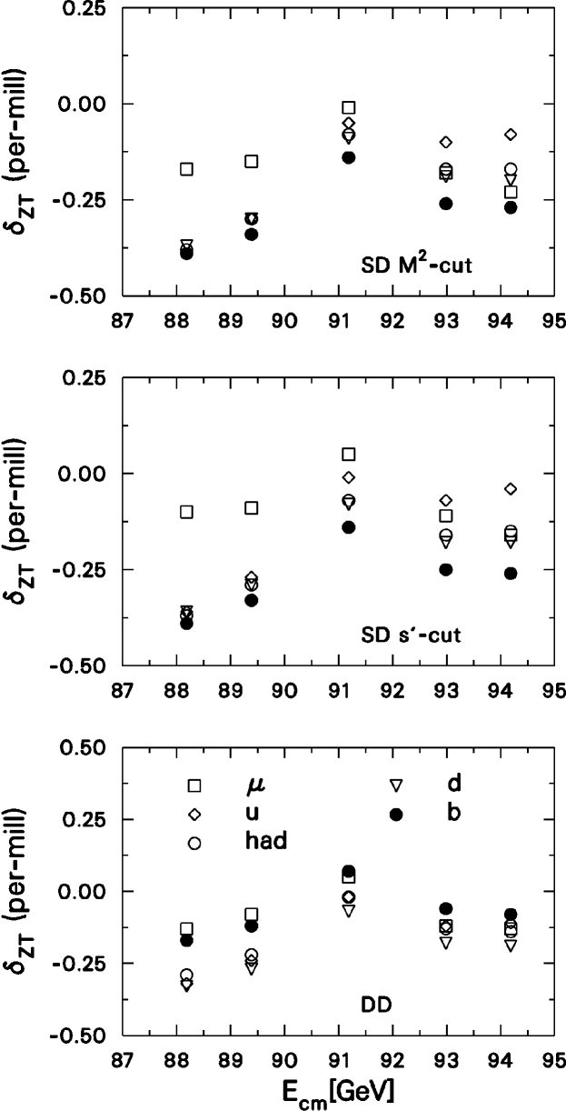
Figure 1: Relative deviations between TOPAZ0 and ZFITTER for total fermionic cross-section. DD-mode is shown with SD-modes corresponding to no-cut or a $M^{2}(f\overline{f})$-cut of $0.01\,s$.

5.2 De-Convoluted Asymmetries

In Tab.(14) we show DD and SD modes for the de-convoluted muonic and heavy quark forward-backward asymmetries.

	Centre-of-mass energy in GeV
	$M_{{}_{Z}}-3$	$M_{{}_{Z}}-1.8$	$M_{{}_{Z}}$	$M_{{}_{Z}}+1.8$	$M_{{}_{Z}}+3$
$A^{\mu}_{{}_{\rm FB}}$ DD	-0.26170	-0.15037	0.01745	0.17510	0.27002
	-0.26167	-0.15037	0.01741	0.17502	0.26991
$A^{\mu}_{{}_{\rm FB}}$ SD – no-cut	-0.26122	-0.15010	0.01742	0.17478	0.26952
	-0.26119	-0.15010	0.01737	0.17469	0.26941
$A^{\mu}_{{}_{\rm FB}}$ SD – $M^{2}$-cut	-0.26128	-0.15013	0.01742	0.17481	0.26958
	-0.26122	-0.15011	0.01738	0.17471	0.26944
$A^{c}_{{}_{\rm FB}}$ DD	-0.09383	-0.02507	0.07411	0.16636	0.22319
	-0.09376	-0.02506	0.07405	0.16624	0.22304
$A^{c}_{{}_{\rm FB}}$ SD – no-cut	-0.08977	-0.02399	0.07092	0.15922	0.21364
	-0.08968	-0.02396	0.07086	0.15909	0.21348
$A^{c}_{{}_{\rm FB}}$ SD – $M^{2}$-cut	-0.08978	-0.02399	0.07093	0.15923	0.21365
	-0.08968	-0.02396	0.07086	0.15910	0.21349
$A^{b}_{{}_{\rm FB}}$ DD	0.03652	0.06403	0.10311	0.13956	0.16242
	0.03615	0.06361	0.10262	0.13903	0.16187
$A^{b}_{{}_{\rm FB}}$ SD – no-cut	0.03556	0.06233	0.10035	0.13579	0.15802
	0.03529	0.06209	0.10014	0.13562	0.15788
$A^{b}_{{}_{\rm FB}}$ SD – $M^{2}$-cut	0.03556	0.06233	0.10035	0.13580	0.15803
	0.03529	0.06209	0.10014	0.13562	0.15788

Table 14: TOPAZ0/ZFITTER comparison of $A^{\mu,c,b}_{{}_{\rm FB}}$ in DD-mode and SD-modes.

In Fig. 2 we show the absolute deviation in per-mill between TOPAZ0 and ZFITTER predictions for the forward-backward asymmetries in DD mode and in SD-modes. From this figure one understands that $A^{b}_{{}_{\rm FB}}$ is indeed the RO showing the largest deviations between the two codes. This is hardly a surprise, given the comparison for $\sin^{2}\theta^{b}_{\rm{eff}}$ reported in Tab.(7). In both cases it is the absence of next-to-leading corrections in the $b\overline{b}$-channel (due to missing non-universal next-to-leading terms) that stays at the root of the relatively large theoretical uncertainty.

For $A^{\mu}_{{}_{\rm FB}}$ the absolute deviations is always below $0.14$ per-mill ($0.04-0.05$ at the peak). For $A^{c}_{{}_{\rm FB}}$ the agreement is also very good, deviations below $0.16$ per-mill (and only at the wings) and peak asymmetries differing of $0.06-0.07$ per-mill. This sort of agreement and consistency between DD-mode and SD-modes shows that also final state QCD corrections are under control in the $c$-channel.

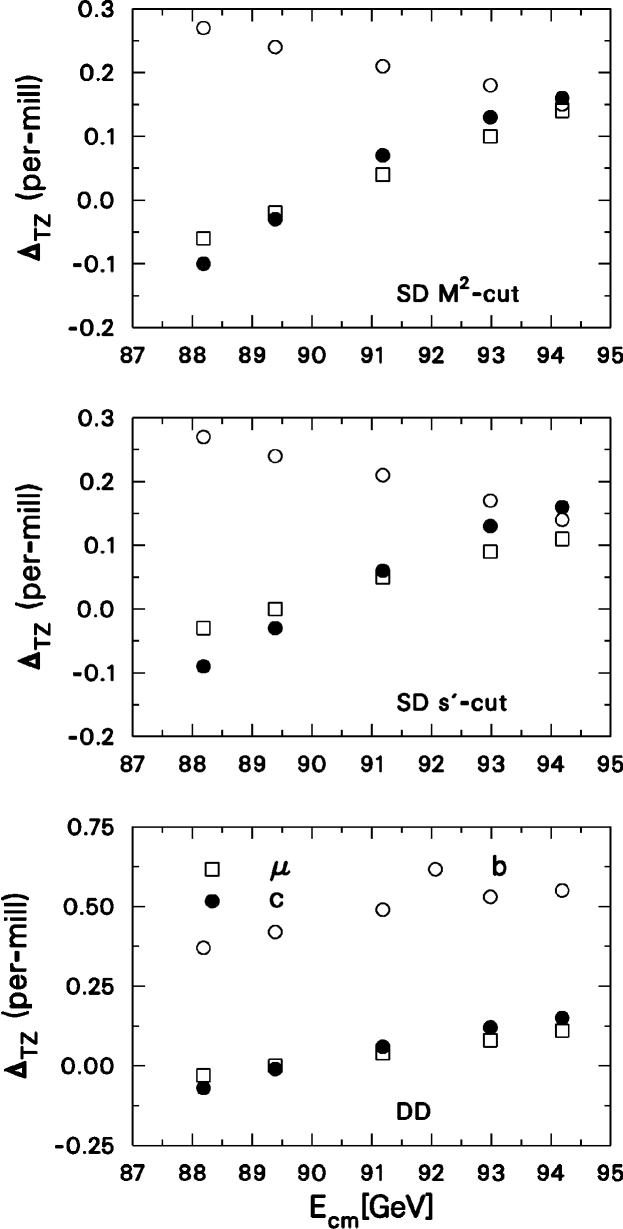
Figure 2: Absolute deviations between TOPAZ0 and ZFITTER for de-convoluted forward-backward asymmetries.

Note that QCD corrections for the forward-backward asymmetry can well be approximated by an expansion in the parameter $x=4m^{2}_{q}/s=4r^{2}\;$,

$$\sigma_{\rm VA}^{q}\to\sigma_{\rm VA}^{q}\,\left(1+\frac{\alpha_{{}_{S}}}{\pi}\,f_{1}\right),$$ (53)

with a correction factor, $f_{1}$, which we write as [26]

$$f_{1}=\frac{8}{3}{x}^{\frac{1}{2}}+\left(\frac{7}{3}+\frac{\pi^{2}}{18}-\frac{2}{3}l_{r}+\frac{1}{3}l_{r}^{2}\right)x-\frac{40}{27}{x}^{\frac{3}{2}}+\left(\frac{55}{24}+\frac{\pi^{2}}{12}-\frac{19}{12}l_{r}+\frac{1}{2}l_{r}^{2}\right)x^{2}+\cdots,$$ (54)

where $l_{r}=\ln r$. These first order corrections vanish in the massless limit. The asymmetry changes as

$$A^{q}_{{}_{\rm FB}}\to A^{q}_{{}_{\rm FB}}\,\left[1-\frac{\alpha_{{}_{S}}}{\pi}\,\left(1-f_{1}\right)\right].$$ (55)

For $b$-quarks the inclusion of QCD final state correction improves the TOPAZ0-ZFITTER agreement. This fact is not completely satisfactory, signalling some difference (and some uncertainty) in the implementation of electroweak/QCD radiative corrections for the $b\overline{b}$-channel.

5.3 Higgs-Mass Dependence of De-Convoluted Observables

Our comparison for de-convoluted ROs has to be extended to a wide range of values for the Higgs boson mass: differences indicate theoretical uncertainties in using the measurements to constrain the mass of the Higgs boson. In Tabs.(15–17) we present cross-sections and asymmetries in the Higgs-mass range $M_{{}_{H}}$ range of $10-1000\,$ GeV. In Fig. 3 we show the relative deviations between the TOPAZ0 and ZFITTER prediction for $\sigma(\mu)$, $\sigma(\rm had)$ and $A^{\mu}_{{}_{\rm FB}}$ in SD no-cut mode as a function of the Higgs mass ranging from $10\,$GeV to $1000\,$GeV.

The figure confirms the good agreement between the two sets of predictions: differences in the peak muonic cross-sections are everywhere below $0.14$ per-mill, reached only at the boundaries of the interval in $M_{{}_{H}}$ ($0.05$ per-mill at $M_{{}_{H}}=100\,$GeV). Deviations in the peak hadronic cross-sections vary from $-0.13$ per-mill at very low values of the Higgs boson mass to $-0.07$ per-mill at $M_{{}_{H}}=100\,$GeV and stay practically constant for higher values of $M_{{}_{H}}$. The variations in relative differences for $\sigma(\mu)$ are $0.09$ per-mill at peak and $0.16,0.11$ per mill at the wings ($M_{{}_{Z}}\pm 3$). For $\sigma_{\rm{had}}$ we have $0.07$ per-mill at peak and $0.17,0.10$ per-mill at the wings. For $A^{\mu}_{{}_{\rm FB}}$ we observe absolute differences which are everywhere below 0.00012 and at the peak below 0.00006.

$\sigma(\mu)$ [nb]
	$M_{{}_{H}}$in GeV
$\sqrt{s}$[GeV]	10	30	100	300	1000
$M_{{}_{Z}}-3$	0.30000	0.30055	0.30055	0.30011	0.29938
	0.30001	0.30059	0.30058	0.30011	0.29937
$M_{{}_{Z}}-1.8$	0.65724	0.65832	0.65839	0.65766	0.65643
	0.65726	0.65839	0.65845	0.65766	0.65641
$M_{{}_{Z}}$	2.00558	2.00613	2.00711	2.00827	0.20098
	2.00537	2.00601	2.00700	2.00809	0.20095
$M_{{}_{Z}}+1.8$	0.65810	0.65968	0.65978	0.65900	0.65772
	0.65815	0.65976	0.65985	0.65902	0.65773
$M_{{}_{Z}}+3$	0.31003	0.31102	0.31104	0.31053	0.30971
	0.31007	0.31107	0.31108	0.31054	0.30973

Table 15: TOPAZ0/ZFITTER comparison for the muonic cross-section in SD fully extrapolated mode for different values of the Higgs boson mass.

$\sigma(\rm had)$ [nb]
	$M_{{}_{H}}$in GeV
$\sqrt{s}$[GeV]	10	30	100	300	1000
$M_{{}_{Z}}-3$	5.99467	6.00515	6.00291	5.99098	5.97237
	5.99740	6.00774	6.00518	5.99267	5.97414
$M_{{}_{Z}}-1.8$	13.40951	13.42945	13.42550	13.40383	13.37020
	13.41443	13.43405	13.42948	13.40683	13.37339
$M_{{}_{Z}}$	41.42574	41.42837	41.43114	41.43364	41.43777
	41.43106	41.43209	41.43401	41.43645	41.44034
$M_{{}_{Z}}+1.8$	13.48804	13.51762	13.51353	13.49007	13.45456
	13.49074	13.52007	13.51559	13.49146	13.45640
$M_{{}_{Z}}+3$	6.26327	6.28209	6.27961	6.26553	6.24431
	6.26441	6.28316	6.28050	6.26606	6.24513

Table 16: TOPAZ0/ZFITTER comparison for the hadronic cross-section in SD fully extrapolated mode for different values of the Higgs boson mass.

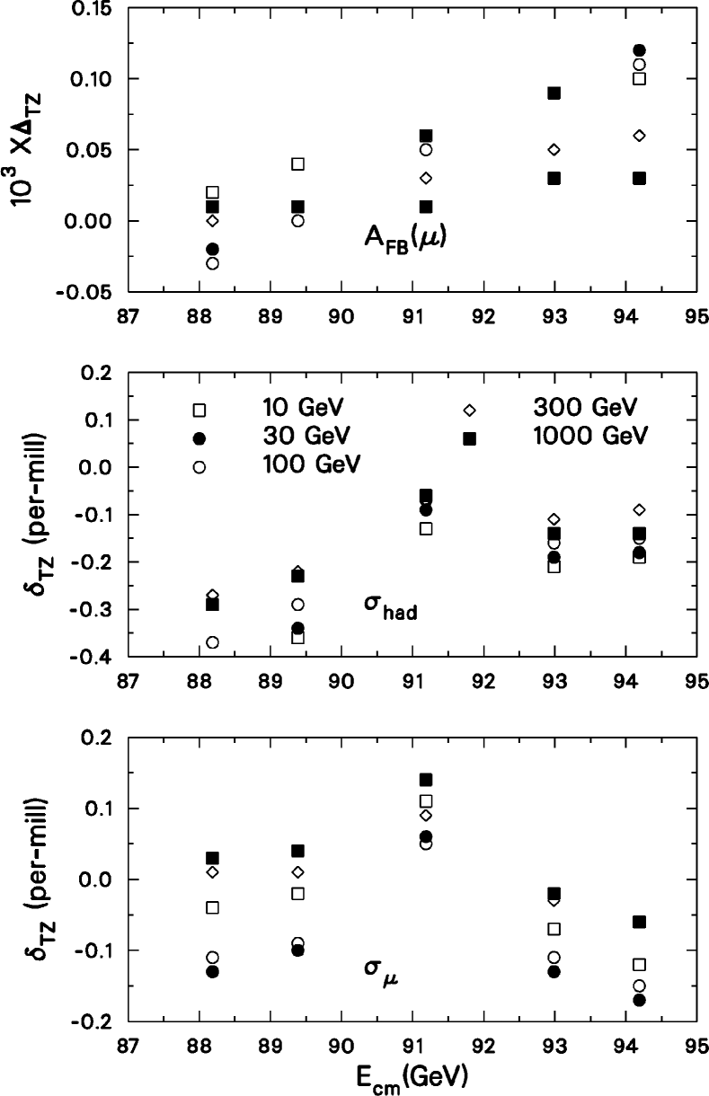
Figure 3: Relative deviations between TOPAZ0 and ZFITTER for $\sigma(\mu)$, $A^{\mu}_{{}_{\rm FB}}$ and $\sigma(\rm had)$ for different values of the Higgs boson mass in SD no-cut mode.

$A^{\mu}_{{}_{\rm FB}}$
	$M_{{}_{H}}$in GeV
$\sqrt{s}$[GeV]	10	30	100	300	1000
$M_{{}_{Z}}-3$	-0.25984	-0.26021	-0.26122	-0.26246	-0.26398
	-0.25986	-0.26019	-0.26119	-0.26246	-0.26399
$M_{{}_{Z}}-1.8$	-0.14864	-0.14909	-0.15010	-0.15126	-0.15264
	-0.14868	-0.14910	-0.15010	-0.15127	-0.15265
$M_{{}_{Z}}$	0.01899	0.01838	0.01742	0.01644	0.01534
	0.01893	0.01832	0.01737	0.01641	0.01533
$M_{{}_{Z}}+1.8$	0.17648	0.17566	0.17478	0.17401	0.17324
	0.17639	0.17557	0.17469	0.17396	0.17321
$M_{{}_{Z}}+3$	0.27130	0.27035	0.26952	0.26890	0.26833
	0.27120	0.27023	0.26941	0.26884	0.26830

Table 17: TOPAZ0/ZFITTER comparison for the muonic forward-backward asymmetry in SD fully extrapolated mode for different values of the Higgs boson mass.

5.4 Standard Model Remnants

POs are determined by fitting ROs, but actually something is still taken from the SM (imaginary parts, parts which have been moved to interference terms and photon-exchange terms) making the model-independent results dependent on the SM. How complicated is such a description? Within the codes we consider sub-contributions to the DD de-convoluted quantities, 1) total DD, 2) DD with $Z$ exchange only, 3) DD with $Z\oplus\gamma$ without interference. For instance we construct the relative and absolute differences

$$\delta^{\rm int}\sigma = {{\sigma^{\rm DD}_{\rm T}}\over{\sigma^{\rm DD}_{Z+\gamma}}}-1\qquad\mbox{in percent},$$

$$\Delta^{\rm int}A^{\mu}_{{}_{\rm FB}} = A^{\mu,\rm DD}_{{}_{\rm FB}}-\left(A^{\mu,\rm DD}_{{}_{\rm FB}}\right)_{Z+\gamma}.$$ (56)

They are reported in Tab.(19). The effect of the $Z-\gamma$ interference is negative below the peak, vanishingly small around it and turning positive and large above it. The effect of $Z-\gamma$ interference is particularly important for the forward-backward asymmetry, as its energy dependence is governed by this interference.

	Centre-of-mass energy in GeV
	$M_{{}_{Z}}-3$	$M_{{}_{Z}}-1.8$	$M_{{}_{Z}}$	$M_{{}_{Z}}+1.8$	$M_{{}_{Z}}+3$
$\delta^{\rm int}\sigma_{\mu}$	$-0.209\,\%$	$-0.136\,\%$	$-0.028\,\%$	$+0.072\,\%$	$+0.132\,\%$
$\delta^{\rm int}\sigma_{\rm had}$	$-0.492\,\%$	$-0.301\,\%$	$-0.029\,\%$	$+0.226\,\%$	$+0.384\,\%$
$\Delta^{\rm int}A^{\mu}_{{}_{\rm FB}}$	-0.27703	-0.16611	0.00145	0.15923	0.25441

Table 18: TOPAZ0 relative differences $\delta^{\rm int}\sigma$ and absolute differences $\Delta^{\rm int}A^{\mu}_{{}_{\rm FB}}$.

	Centre-of-mass energy in GeV
	$M_{{}_{Z}}-3$	$M_{{}_{Z}}-1.8$	$M_{{}_{Z}}$	$M_{{}_{Z}}+1.8$	$M_{{}_{Z}}+3$
$\sigma_{\mu}\,$[nb] No Ims	0.29996	0.65713	2.00343	0.65855	0.31045
$\sigma_{\mu}\,$[nb]	0.29999	0.65718	2.00341	0.65856	0.31047
Diff.[pb]	+0.03	+0.05	-0.02	-0.01	+0.02
$\sigma_{\rm had}\,$[nb] No Ims	5.78583	12.94061	39.93848	13.02635	6.05322
$\sigma_{\rm had}\,$[nb]	5.78492	12.93841	39.92967	13.02421	6.05233
Diff.[pb]	-0.91	-2.20	-8.81	-2.14	-0.89
$A^{\mu}_{{}_{\rm FB}}$ No Ims	-0.26311	-0.15181	0.01598	0.17364	0.26858
$A^{\mu}_{{}_{\rm FB}}$	-0.26170	-0.15037	0.01745	0.17510	0.27002
Diff.	-0.00141	-0.00144	-0.00147	+0.00146	-0.00144

Table 19: TOPAZ0 comparison of DD (completely de-convoluted) RO with/without imaginary parts (Ims) in couplings and form factors.

Among the de-convoluted quantities the most relevant are those computed at $s=M^{2}_{{}_{Z}}$, which have an obvious counterpart in the PO, that we have already computed, i.e., $\sigma^{0}_{\ell}\,$, $\sigma^{0}_{{h}}\,$, and $A^{0,\rm l}_{{}_{\rm FB}}$.

There is however a noticeable difference between the two sets, represented by the interference of the $Z-\gamma$ $s$-channel diagrams, including the imaginary parts in $\alpha(s)$ and in the form-factors, the latter being particularly relevant for the leptonic forward-backward asymmetry. This effect is illustrated in Tab.(19).

5.5 The $Z-\gamma$ Interference for Cross-Sections

One must evaluate the residual SM dependence of the so-called model-independent parameters; one simple source of such a SM dependence is due to the interference terms for cross-sections, which are governed by the value of $\sin^{2}\theta^{\rm lept}_{\rm{eff}}$ and therefore depend on the values of $m_{t}$ and $M_{{}_{H}}$ chosen. Note that for leptonic final states, one can use the POs to express the interference terms, at least up to imaginary parts which must be taken from the SM as usual. This is possible because the interference terms are proportional to the effective couplings which can be derived from the POs $R_{\ell}$ and $A^{0,\ell}_{{}_{\rm FB}}$. However, for the inclusive hadronic final state, which is a sum over the five light quark flavours, the interference terms must be taken completely from the SM.

	Centre-of-mass energy in GeV
$M_{{}_{H}}\,$[GeV]	$M_{{}_{Z}}-3$	$M_{{}_{Z}}-1.8$	$M_{{}_{Z}}$	$M_{{}_{Z}}+1.8$	$M_{{}_{Z}}+3$
$\delta^{\rm int}\sigma_{\mu}$
10	$-0.229\,\%$	$-0.150\,\%$	$-0.030\,\%$	$+0.082\,\%$	$+0.149\,\%$
100	$-0.209\,\%$	$-0.136\,\%$	$-0.028\,\%$	$+0.072\,\%$	$+0.132\,\%$
1000	$-0.181\,\%$	$-0.119\,\%$	$-0.026\,\%$	$+0.060\,\%$	$+0.111\,\%$
$\delta^{\rm int}\sigma_{\rm had}$
10	$-0.518\,\%$	$-0.317\,\%$	$-0.029\,\%$	$+0.240\,\%$	$+0.407\,\%$
100	$-0.492\,\%$	$-0.301\,\%$	$-0.029\,\%$	$+0.226\,\%$	$+0.384\,\%$
1000	$-0.457\,\%$	$-0.281\,\%$	$-0.028\,\%$	$+0.207\,\%$	$+0.353\,\%$

Table 20: TOPAZ0 relative differences $\delta^{\rm int}\sigma(M_{{}_{H}})=\sigma^{\rm DD}/\sigma^{\rm DD}_{{\scriptscriptstyle{Z}}+\gamma}-1$ as a function of the Higgs boson mass in DD-mode.

In Tab.(20) we show the relative deviation of excluding/including the $Z-\gamma$ interference as a function of the Higgs boson mass in DD-mode. As observed before the $Z-\gamma$ interference is negative below the peak and changes sign above it. It is vanishingly small at the resonance for all values of $M_{{}_{H}}$, approximately $-0.03\%$, and can be sizeable at the wings, $-0.2\%(-0.5\%)$ at the left wing and $+0.1\%(+0.4\%)$ at the right wing for the muonic (hadronic) cross-section. The Higgs-mass dependence of the $Z-\gamma$ interference is rather large, up to 20% of the interference itself.

6 Convoluted Realistic Observables

6.1 Comparison for Extrapolated Setup

Having discussed the status of our comparisons before the introduction of initial-state QED radiation we now proceed to comparing the convoluted quantities and the effect of convolution.

The default of TOPAZ0/ZFITTER is to account for initial-state QED radiation through a so-called additive formulation of the QED radiator (flux-function), which is a mixture of leading-logarithms (LL) and finite-order results. In [30] a proof is given that the $\beta x^{\beta-1}$ term should be factorized in front of, at least, the LL component. This result is obtained up to third order LL, and there are good indications from fourth and fifth orders that it is true to infinite order. Recently explicit $\alpha^{3}L^{3}$ terms became known [30] and also [31]. For higher orders we refer to [32] and [33]. In TOPAZ0/ZFITTER the ${\mathcal{O}}\left(\alpha^{3}\right)$ radiator is implemented according to [34]. Recently TOPAZ0 and ZFITTER have implemented the order $\alpha^{3}$ factorized (YFS) radiator as reported in [35].

There is a pattern of convolution that we want to compare in our step-by-step procedure.

• Complete RO, with QED initial state radiation implemented through an additive ${\mathcal{O}}\left(\alpha^{3}\right)$ radiator [34].

• Complete RO, with QED initial state radiation implemented through a factorized ${\mathcal{O}}\left(\alpha^{3}\right)$ radiator [35].

The following two equations define cross-sections and forward-backward asymmetries convoluted with ISR:

$$\sigma_{{}_{\rm T}}\left(s\right)=\int^{1}_{z_{{}_{0}}}\,dzH\left({z;s}\right){\hat{\sigma}}_{{}_{\rm T}}\bigl{(}zs\bigr{)},$$ (57)

where $z_{{}_{0}}=s_{0}/s$ and

$$A_{{}_{\rm FB}}\left(s\right)=\frac{\pi\alpha^{2}Q^{2}_{e}Q^{2}_{f}}{\sigma_{\rm tot}}\,\int^{1}_{z_{{}_{0}}}\,dz\frac{1}{\left(1+z\right)^{2}}\,H_{{}_{\rm FB}}\left(z;s\right)\,{\hat{\sigma}}_{{}_{\rm FB}}\bigl{(}zs\bigr{)},$$ (58)

Note that the so-called radiator (or flux function), $H\left({z;s}\right)$, is known up to terms of order $\alpha^{3}$ while $H_{{}_{\rm FB}}$ is only known up to terms of order $\alpha^{2}$.

The kernel cross-sections ${\hat{\sigma}}_{{}_{\rm T,FB}}$ should be understood as the improved Born approximation (IBA), including imaginary parts and corrected with all electroweak and possibly all FSR (QED $\,\otimes\,$QCD) corrections where all coupling constants and effective vector and axial weak couplings are running, i.e., they depend on $s^{\prime}=zs$ under the convolution integrals in Eq.(57) and Eq.(58). In practice this takes a lot of CPU time and for this reason some time-saving options are foreseen in the codes. For instance, one may calculate effective weak couplings only once at $s$ rather than at $s^{\prime}$ thereby saving a conspicuous amount of CPU time.

We study the accuracy of such approximations with ${\tt ZFITTER}$. In Tab. 21 we report ROs calculated with no convolution at all (all couplings evaluated at $s$), convolution of $\alpha$ only ($\alpha(s)\to\alpha(s^{\prime})$), and full convolution of all electroweak radiative corrections; corresponding to the ZFITTER flag CONV with values CONV=0,1,2, respectively. The bulk of the running-couplings effect is given by the $\alpha$ convolution, in particular below the wing. The remaining effect is totally negligible at the resonance and below, growing to $\sim-0.15$ per-mill above the resonance for cross-sections and remaining negligible for the asymmetries. This study proves that one may avoid using the CPU-time consuming full convolution of all electroweak radiative corrections and that it is sufficient to keep the $\alpha$ convolution only. This is the default used for the ZFITTER numbers reported in this article.

In TOPAZ0 all universal electroweak corrections and final-state QCD corrections are put in convolution with initial-state QED radiation and therefore the couplings, $\alpha$, and $\alpha_{{}_{S}}$ are evaluated at the scale $s^{\prime}$. Weak boxes, vertices and expanded bosonic self-energy corrections are added linearly, evaluated at the nominal energy. The latter is also true for IFI.

Results are shown in Tab.(22) where we include all steps in the process de-convoluted $\,\to\,$ convoluted, i.e., DD, SD, CA3 and CF3. The reported results refer to an $M^{2}(f\overline{f})$ cut of $0.01\,s$. The relative deviations between TOPAZ0 and ZFITTER are shown in Fig. 4. The numbers of Tab.(22) are produced with a $M^{2}(f\overline{f})$-cut of $0.01\,s$. It is instructive to compare with similar results obtained by imposing the an $s^{\prime}$-cut, e.g. $s^{\prime}\geq 0.01\,s$. The comparison is shown in Tab.(23) and Fig. 5. From Tab.(23) one sees that the differences between the two cuts are of $0.43\,(1.38)\,$pb for the muonic (hadronic) peak cross-section. There is really no problem as long as the procedure is fully specified.

It emerges from this comparisons that the agreement for the muonic cross-section for energies below the peak is quite reasonable but less satisfactory than for hadrons. Given the agreement at the level of de-convoluted cross-sections and once we have observed that the de-convolution is satisfactory for hadrons, we come to the conclusion that for muons the low-$q^{2}$ region, where the Coulomb pole and mass effects (for very loose $s^{\prime}$-cuts) may become relevant, gives the dominant difference in $\sigma_{\mu}$.

	Centre-of-mass energy in GeV
	$M_{{}_{Z}}-3$	$M_{{}_{Z}}-1.8$	$M_{{}_{Z}}$	$M_{{}_{Z}}+1.8$	$M_{{}_{Z}}+3$
$\sigma_{\mu}\,$[nb]	0.22862	0.47672	1.48012	0.69526	0.40655
	0.22843	0.47653	1.47995	0.69509	0.40638
	0.22842	0.47653	1.47992	0.69505	0.40633
	-0.04	0	-0.02	-0.06	-0.12
$\sigma_{\rm had}\,$[nb]	4.45219	9.60235	30.43892	14.18454	8.19986
	4.45146	9.60165	30.43824	14.18391	8.19923
	4.45130	9.60139	30.43753	14.18270	8.19791
	-0.04	-0.03	-0.02	-0.09	-0.16
$A^{\mu}_{{}_{\rm FB}}$	-0.28308	-0.16979	-0.00066	0.11177	0.15451
	-0.28330	-0.16985	-0.00066	0.11182	0.15461
	-0.28330	-0.16985	-0.00066	0.11183	0.15464
	0	0	0	+0.01	+0.03

Table 21: ZFITTER illustration of the effect of convolution of electroweak radiative corrections in CA3 mode with a cut of $s^{\prime}>0.01s$. First line is no convolution, second line is $\alpha(s)\to\alpha(s^{\prime})$ convolution, third line is full convolution of all electroweak radiative corrections. Fourth line is difference between third and second line.

	Centre-of-mass energy in GeV
	$M_{{}_{Z}}-3$	$M_{{}_{Z}}-1.8$	$M_{{}_{Z}}$	$M_{{}_{Z}}+1.8$	$M_{{}_{Z}}+3$
$\sigma_{\mu}\,$[nb] DD	0.29999	0.65718	2.00341	0.65856	0.31047
	0.30003	0.65724	2.00331	0.65863	0.31051
$\sigma_{\mu}\,$[nb] SD	0.30047	0.65821	2.00656	0.65960	0.31095
	0.30052	0.65832	2.00659	0.65971	0.31102
$\sigma_{\mu}\,$[nb] CA3	0.22840	0.47642	1.47967	0.69490	0.40628
	0.22836	0.47641	1.47962	0.69492	0.40627
$\sigma_{\mu}\,$[nb] CF3	0.22841	0.47645	1.47977	0.69495	0.40630
	0.22837	0.47644	1.47971	0.69497	0.40629
$\sigma_{\rm had}\,$[nb] DD	5.78492	12.93841	39.92967	13.02421	6.05233
	5.78670	12.94148	39.93079	13.02591	6.05313
$\sigma_{\rm had}\,$[nb] SD	6.00265	13.42490	41.42929	13.51293	6.27933
	6.00500	13.42901	41.43272	13.51517	6.28030
$\sigma_{\rm had}\,$[nb] CA3	4.44990	9.59865	30.43501	14.18203	8.19853
	4.45129	9.60132	30.43725	14.18342	8.19894
$\sigma_{\rm had}\,$[nb] CF3	4.45016	9.59921	30.43696	14.18307	8.19901
	4.45157	9.60191	30.43929	14.18451	8.19945
$A^{\mu}_{{}_{\rm FB}}$ DD	-0.26170	-0.15037	0.01745	0.17510	0.27002
	-0.26167	-0.15037	0.01741	0.17502	0.26991
$A^{\mu}_{{}_{\rm FB}}$ SD	-0.26128	-0.15013	0.01742	0.17481	0.26958
	-0.26122	-0.15011	0.01738	0.17471	0.26944
$A^{\mu}_{{}_{\rm FB}}$ CA3	-0.28321	-0.16981	-0.00062	0.11189	0.15470
	-0.28336	-0.16988	-0.00066	0.11184	0.15464
$A^{\mu}_{{}_{\rm FB}}$ CF3	-0.28320	-0.16980	-0.00062	0.11189	0.15469
	-0.28340	-0.16990	-0.00066	0.11185	0.15465

Table 22: TOPAZ0/ZFITTER comparison of complete RO (CA3 and CF3) with DD and SD ($M^{2}$-cut) modes.

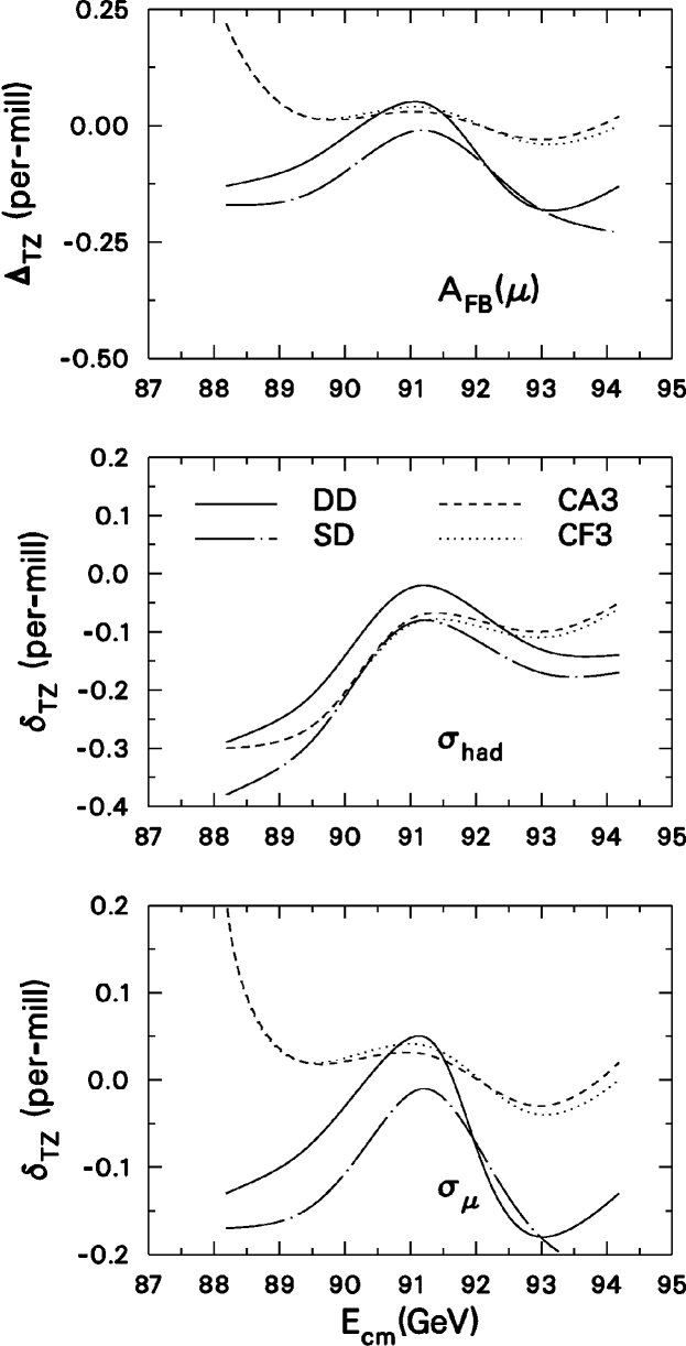
Figure 4: Relative deviations between TOPAZ0 and ZFITTER for muonic and hadronic cross-section in DD, SD, CA3 and CF3 modes. The last three are corresponding to a cut $M^{2}(f\overline{f})$ of $0.01\,s$.

	Centre-of-mass energy in GeV
	$M_{{}_{Z}}-3$	$M_{{}_{Z}}-1.8$	$M_{{}_{Z}}$	$M_{{}_{Z}}+1.8$	$M_{{}_{Z}}+3$
$\sigma_{\mu}\,$[nb] DD	0.29999	0.65718	2.00341	0.65856	0.31047
	0.30003	0.65724	2.00331	0.65863	0.31051
$\sigma_{\mu}\,$[nb] SD	0.30055	0.65839	2.00711	0.65978	0.31104
	0.30058	0.65844	2.00700	0.65985	0.31108
$\sigma_{\mu}\,$[nb] CA3	0.22849	0.47657	1.48010	0.69512	0.40642
	0.22843	0.47653	1.47995	0.69509	0.40638
$\sigma_{\mu}\,$[nb] CF3	0.22850	0.47660	1.48019	0.69517	0.40644
	0.22844	0.47656	1.48004	0.69514	0.40640
$\sigma_{\rm had}\,$[nb] DD	5.78492	12.93841	39.92967	13.02421	6.05233
	5.78670	12.94148	39.93079	13.02591	6.05313
$\sigma_{\rm had}\,$[nb] SD	6.00291	13.42550	41.43114	13.51353	6.27961
	6.00518	13.42948	41.43401	13.51559	6.28050
$\sigma_{\rm had}\,$[nb] CA3	4.45012	9.59910	30.43639	14.18269	8.19892
	4.45146	9.60165	30.43824	14.18391	8.19923
$\sigma_{\rm had}\,$[nb] CF3	4.45038	9.59966	30.43834	14.18373	8.19940
	4.45174	9.60225	30.44028	14.18499	8.19974
$A^{\mu}_{{}_{\rm FB}}$ DD	-0.26170	-0.15037	0.01745	0.17510	0.27002
	-0.26167	-0.15037	0.01741	0.17502	0.26991
$A^{\mu}_{{}_{\rm FB}}$ SD	-0.26122	-0.15010	0.01742	0.17478	0.26952
	-0.26119	-0.15010	0.01737	0.17469	0.26941
$A^{\mu}_{{}_{\rm FB}}$ CA3	-0.28312	-0.16977	-0.00062	0.11186	0.15466
	-0.28330	-0.16985	-0.00066	0.11182	0.15461
$A^{\mu}_{{}_{\rm FB}}$ CF3	-0.28311	-0.16976	-0.00062	0.11186	0.15465
	-0.28333	-0.16987	-0.00066	0.11183	0.15462

Table 23: TOPAZ0/ZFITTER comparison of complete RO (CA3 and CF3) with DD and SD ($s^{\prime}$-cut) modes.

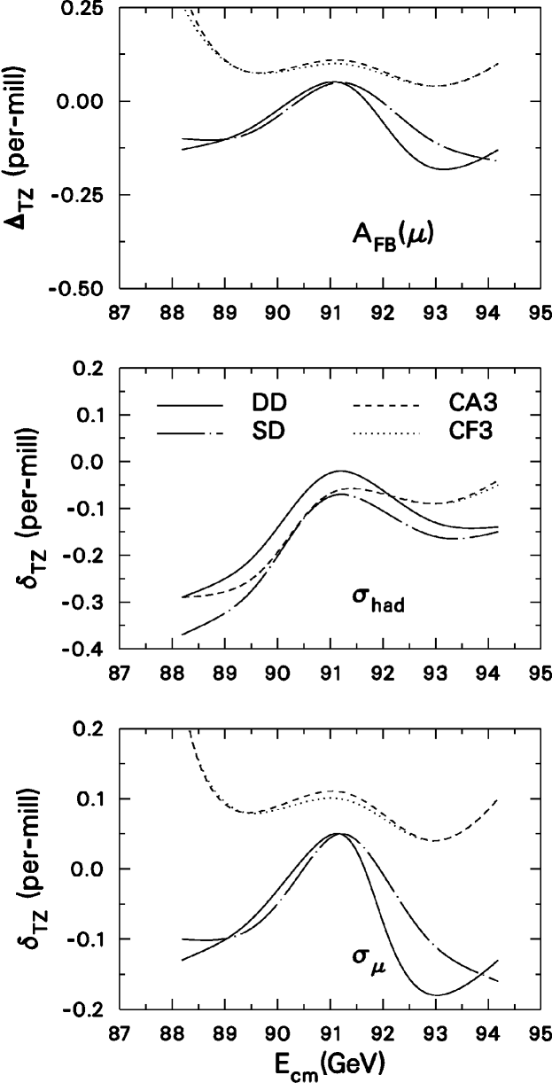
Figure 5: Relative deviations between TOPAZ0 and ZFITTER for muonic and hadronic cross-section in DD, SD, CA3 and CF3 modes. The last three are corresponding to a cut on $s^{\prime}$ of $0.01\,s$.

The effect of moving the $s^{\prime}$-cut from $0.01\,s$ to $0.1\,s$ is shown in Tab.(24). As a result the agreement becomes much better, especially on the lower tail of the resonance. This fact is also shown in Fig. 6.

	Centre-of-mass energy in GeV
	$M_{{}_{Z}}-3$	$M_{{}_{Z}}-1.8$	$M_{{}_{Z}}$	$M_{{}_{Z}}+1.8$	$M_{{}_{Z}}+3$
$\sigma_{\mu}\,$[nb] SD	0.30055	0.65839	2.00711	0.65978	0.31104
	0.30058	0.65845	2.00700	0.65985	0.31108
$\sigma_{\mu}\,$[nb] CA3	0.22849	0.47657	1.48010	0.69512	0.40642
	0.22843	0.47653	1.47995	0.69509	0.40638
	0.22674	0.47487	1.47845	0.69353	0.40487
	0.22674	0.47489	1.47836	0.69356	0.40489
$A^{\mu}_{{}_{\rm FB}}$ SD	-0.26122	-0.15010	0.01742	0.17478	0.26952
	-0.26119	-0.15010	0.01737	0.17469	0.26941
$A^{\mu}_{{}_{\rm FB}}$ CA3	-0.28312	-0.16977	-0.00062	0.11186	0.15466
	-0.28330	-0.16985	-0.00066	0.11182	0.15461
	-0.28526	-0.17035	-0.00061	0.11214	0.15528
	-0.28532	-0.17040	-0.00064	0.11210	0.15523

Table 24: TOPAZ0/ZFITTER comparison of complete RO (CA3-mode) with SD ($s^{\prime}$-cut) mode. For CA3-mode first (second) row correspond to T(Z) $s^{\prime}>0.01\,s$. Third (fourth) row give instead $s^{\prime}>0.1\,s$.

In Tab.(25) we show the comparison for heavy quark forward-backward asymmetries, including initial-state QED radiation. As we have observed before the $b$-channel shows larger deviations. Even though the agreement for the convoluted $A^{b}_{{}_{\rm FB}}$ is satisfactory, especially at the peak, one should not forget that a similar comparison for DD-de-convoluted $A^{b}_{{}_{\rm FB}}$ is considerably worse so that the result of Tab.(25) is also a consequence of accidental compensations.

	Centre-of-mass energy in GeV
	$M_{{}_{Z}}-3$	$M_{{}_{Z}}-1.8$	$M_{{}_{Z}}$	$M_{{}_{Z}}+1.8$	$M_{{}_{Z}}+3$
$A^{c}_{{}_{\rm FB}}$	-0.10600	-0.03625	0.06068	0.12386	0.14840
	-0.10598	-0.03625	0.06065	0.12377	0.14827
	-0.02	0.00	+0.03	+0.09	+0.13
$A^{b}_{{}_{\rm FB}}$	0.028131	0.05705	0.09611	0.12135	0.13105
	0.028078	0.05701	0.09612	0.12161	0.13169
	+0.05	+0.04	-0.01	-0.26	-0.64

Table 25: TOPAZ0/ZFITTER comparison of heavy quark forward-backward asymmetries in CA3-mode. Third row is the absolute deviation in per-mill.

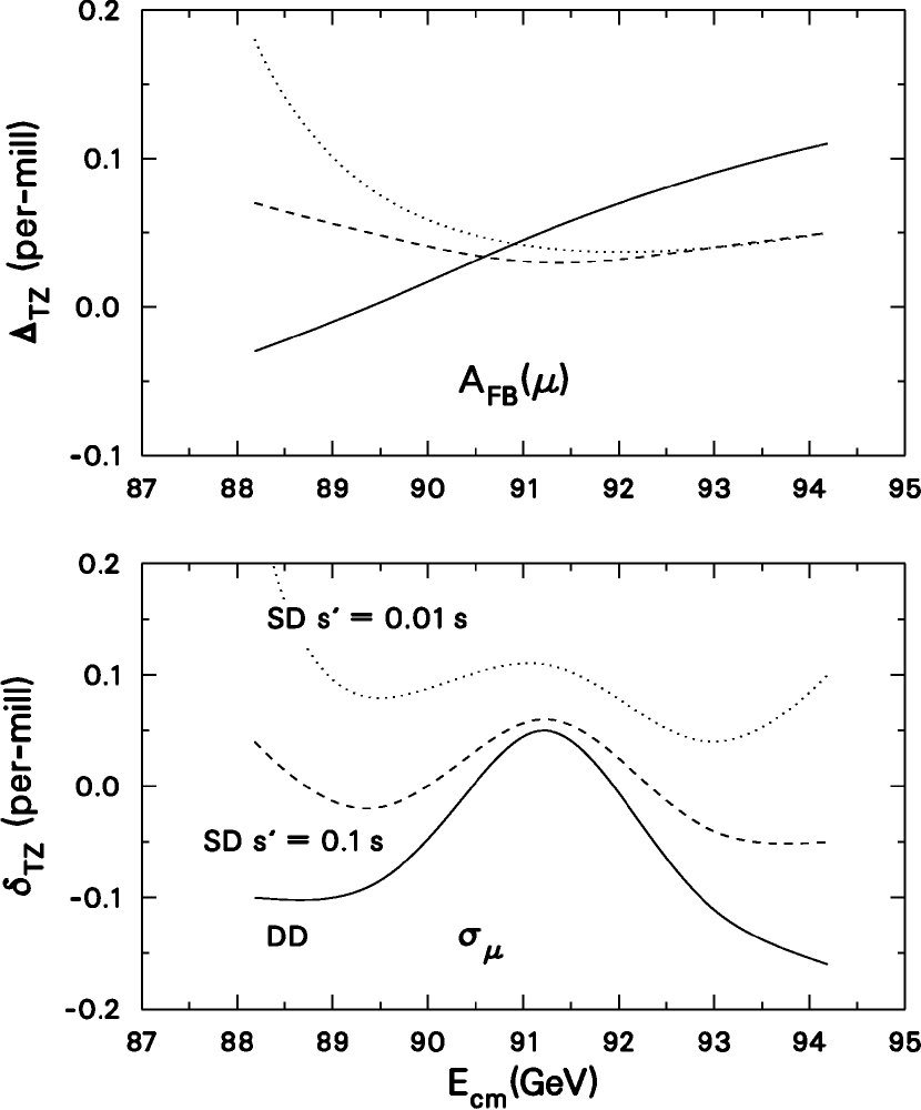
Figure 6: Relative deviations between TOPAZ0 and ZFITTER for muonic total cross-section and forward-backward asymmetry in SD-mode and CA3-mode with two set of $s^{\prime}$-cuts.

6.2 Comparison with Realistic Kinematical Cuts

We have also devoted an effort in order to present the most up-to-date analysis for ROs with realistic kinematical cuts. Therefore, we go beyond the fully extrapolated set-up for muonic channel (with the inclusion of a $s^{\prime}/M^{2}$-cut) by considering

• $e^{+}e^{-}\to\mu^{+}\mu^{-}$ for $\theta_{\rm acc}<\theta_{-}<\pi-\theta_{\rm acc}$ ($\theta_{\rm acc}=0^{\circ},20^{\circ}$ and $40^{\circ}$),
  $\theta_{\rm acoll}<10^{\circ},~{}25^{\circ}$, and $E_{th}(\mu^{\pm})=1\,$GeV,

where $\theta_{-}$ is the final-state fermion scattering angle and $\theta_{\rm acoll}$ the acollinearity between the final-state fermions. The results are shown in Tabs.(26–27).

	$\theta_{\rm acc}$	Centre-of-mass energy in GeV
		$M_{{}_{Z}}-3$	$M_{{}_{Z}}-1.8$	$M_{{}_{Z}}$	$M_{{}_{Z}}+1.8$	$M_{{}_{Z}}+3$
$\sigma_{\mu}\,$[nb]	$0^{\circ}$	0.21932	0.46287	1.44795	0.67725	0.39366
		0.21928	0.46285	1.44781	0.67722	0.39361
		+0.18	+0.04	+0.10	+0.04	+0.13
	$20^{\circ}$	0.19990	0.42207	1.32066	0.61759	0.35886
		0.19987	0.42205	1.32053	0.61756	0.35881
		+0.15	+0.05	+0.10	+0.05	+0.14
	$40^{\circ}$	0.15034	0.31762	0.99428	0.46479	0.26989
		0.15032	0.31760	0.99415	0.46474	0.26983
		+0.13	+0.06	+0.13	+0.11	+0.22
$A^{\mu}_{{}_{\rm FB}}$	$0^{\circ}$	-0.28450	-0.16914	0.00033	0.11512	0.16107
		-0.28453	-0.16911	0.00025	0.11486	0.16071
		+0.03	-0.03	+0.08	+0.26	+0.36
	$20^{\circ}$	-0.27509	-0.16352	0.00042	0.11171	0.15645
		-0.27506	-0.16347	0.00035	0.11148	0.15616
		-0.03	-0.05	+0.07	+0.23	+0.29
	$40^{\circ}$	-0.24219	-0.14396	0.00054	0.09906	0.13903
		-0.24207	-0.14386	0.00050	0.09893	0.13891
		-0.12	-0.10	+0.04	+0.13	+0.12

Table 26: TOPAZ0/ZFITTER comparison for muonic total cross-section and forward-backward asymmetry of complete RO (CA3-mode) with the angular acceptance ($\theta_{\rm acc}=0^{\circ},10^{\circ},20^{\circ}$) and acollinearity ($\theta_{\rm acol}<10^{\circ}$) cuts. First row TOPAZ0, second row ZFITTER, third row relative (absolute) deviations in per-mill.

We register an agreement comparable with the one obtained with $s^{\prime}/M^{2}$-cut, perhaps deteriorating a little for $A^{\mu}_{{}_{\rm FB}}$ at the wings. In conclusion the agreement between TOPAZ0 and ZFITTER remains rather remarkable even when the geometrical acceptance is constrained and also final-state energies and the acollinearity angle are bounded.

	$\theta_{\rm acc}$	Centre-of-mass energy in GeV
		$M_{{}_{Z}}-3$	$M_{{}_{Z}}-1.8$	$M_{{}_{Z}}$	$M_{{}_{Z}}+1.8$	$M_{{}_{Z}}+3$
$\sigma_{\mu}\,$[nb]	$0^{\circ}$	0.22333	0.46971	1.46611	0.68690	0.40034
		0.22328	0.46968	1.46598	0.68688	0.40031
		+0.22	+0.06	+0.09	+0.03	+0.075
	$20^{\circ}$	0.20359	0.42835	1.33731	0.62648	0.36507
		0.20357	0.42833	1.33718	0.62647	0.36505
		+0.10	+0.05	+0.10	+0.02	+0.055
	$40^{\circ}$	0.15320	0.32245	1.00698	0.47167	0.27479
		0.15318	0.32243	1.00682	0.47164	0.27477
		+0.13	+0.06	+0.16	+0.06	+0.07
$A^{\mu}_{{}_{\rm FB}}$	$0^{\circ}$	-0.28617	-0.17037	-0.00032	0.11324	0.15730
		-0.28647	-0.17049	-0.00043	0.11293	0.15682
		+0.30	+0.12	+0.11	+0.31	+0.48
	$20^{\circ}$	-0.27695	-0.16485	-0.00026	0.10974	0.15250
		-0.27722	-0.16497	-0.00037	0.10944	0.15204
		+0.27	+0.12	+0.11	+0.30	+0.46
	$40^{\circ}$	-0.24423	-0.14536	-0.00016	0.09703	0.13492
		-0.24445	-0.14545	-0.00026	0.09678	0.13454
		+0.22	+0.09	+0.10	+0.25	+0.38

Table 27: The same as in Tab. 26 but for the acollinearity cut $\theta_{\rm acol}<25^{\circ}$.

We note that the coding in ZFITTER, for the part involving realistic cuts, is based on some old work [36]. A recent study, presented in [37], shows that the approximations made in the former reference ensure sufficient technical precision of the treatment of ISR, ${\mathcal{O}}\left(10^{-4}\right)$, at SLD/LEP-1 energies. (See Section 7 for the situation concerning initial-final QED interference). Coding in TOPAZ0 is always based on the work of [23].

6.3 Uncertainty on QED Convolution

We now return to a detailed analysis of initial-state QED radiation by defining convolution factors for each realistic observable $O$, giving the net effect of initial-state QED radiation at the various energies.

$$\delta^{\rm dec}\left(O\right)=\frac{O}{O^{\rm SD}}-1,\qquad\Delta^{\rm dec}\left(O\right)=O-O^{\rm SD}.$$ (59)

For convenience of the reader we reproduce in Tab.(28) the results for the CA3 and CF3 mode. From Tab.(28) we derive the absolute differences, for $A^{\mu}_{{}_{\rm FB}}$, and the relative ones, for cross-sections, between additive and factorized versions of the QED radiators. They are shown in Tab.(29).

	Centre-of-mass energy in GeV
	$M_{{}_{Z}}-3$	$M_{{}_{Z}}-1.8$	$M_{{}_{Z}}$	$M_{{}_{Z}}+1.8$	$M_{{}_{Z}}+3$
$\delta^{\rm dec}(\sigma^{\rm CA3}_{\mu})$ T	-23.976	-27.616	-26.257	5.356	30.665
$\delta^{\rm dec}(\sigma^{\rm CA3}_{\mu})$ Z	-24.007	-27.629	-26.261	5.341	30.631
$\delta^{\rm dec}(\sigma^{\rm CF3}_{\mu})$ T	-23.973	-27.611	-26.253	5.364	30.671
$\delta^{\rm dec}(\sigma^{\rm CF3}_{\mu})$ Z	-24.000	-27.624	-26.256	5.348	30.637
$\delta^{\rm dec}(\sigma^{\rm CA3}_{\rm had})$ T	-25.867	-28.501	-26.537	4.952	30.564
$\delta^{\rm dec}(\sigma^{\rm CA3}_{\rm had})$ Z	-25.873	-28.503	-26.538	4.945	30.550
$\delta^{\rm dec}(\sigma^{\rm CF3}_{\rm had})$ T	-25.863	-28.497	-26.533	4.959	30.572
$\delta^{\rm dec}(\sigma^{\rm CF3}_{\rm had})$ Z	-25.869	-28.499	-26.533	4.953	30.558
$\Delta^{\rm dec}(A^{\mu\rm CA3}_{{}_{\rm FB}})$ T	-2.190	-1.967	-1.804	-6.292	-11.486
$\Delta^{\rm dec}(A^{\mu\rm CA3}_{{}_{\rm FB}})$ Z	-2.211	-1.975	-1.803	-6.287	-11.480
$\Delta^{\rm dec}(A^{\mu\rm CF3}_{{}_{\rm FB}})$ T	-2.189	-1.966	-1.804	-6.292	-11.487
$\Delta^{\rm dec}(A^{\mu\rm CF3}_{{}_{\rm FB}})$ Z	-2.215	-1.977	-1.803	-6.286	-11.479

Table 28: RO: the effect in $\%$ of initial state QED radiation for CA3 and CF3 modes.

	Centre-of-mass energy in GeV
	$M_{{}_{Z}}-3$	$M_{{}_{Z}}-1$	$M_{{}_{Z}}$	$M_{{}_{Z}}+1$	$M_{{}_{Z}}+3$
$10^{4}\times\,$(fact/add-1)
$\sigma_{\mu}$	0.44	0.63	0.61	0.72	0.49
	0.88	0.63	0.68	0.72	0.49
$\sigma_{\rm had}$	0.58	0.58	0.64	0.73	0.59
	0.61	0.62	0.67	0.76	0.62
fact-add [pb]
$\sigma_{\mu}$	0.01	0.03	0.09	0.05	0.02
	0.02	0.03	0.10	0.05	0.02
$\sigma_{\rm had}$	0.26	0.56	1.95	1.04	0.48
	0.27	0.60	2.04	1.08	0.51
$10^{5}\times\,$(fact-add)
$A^{\mu}_{{}_{\rm FB}}$	1.00	1.00	0.00	0.00	-1.00
	-4.00	-2.00	0.00	1.00	1.00

Table 29: Absolute and relative differences in TOPAZ0 and in ZFITTER for additive and factorized radiators.

To give an example of the developments in the treatment of QED initial-state radiation we recall that in TOPAZ0 the following steps have occurred:

• the leading ${\mathcal{O}}\left(\alpha^{2}\right)$ result was considered in version 1.0,

• the complete ${\mathcal{O}}\left(\alpha^{2}\right)$ result, i.e., leading plus NLO ${\mathcal{O}}\left(\alpha^{2}L\right)$ and NNLO ${\mathcal{O}}\left(\alpha^{2}L^{0}\right)$ was added in version 2.0 [38],

• the complete ${\mathcal{O}}\left(\alpha^{2}\right)$ plus leading ${\mathcal{O}}\left(\alpha^{3}L^{3}\right)$ result as been included after version 4.0 [39],

where $L=\ln(s/m^{2}_{e})$. Inserting the ${\mathcal{O}}\left(\alpha^{3}L^{3}\right)$ terms into the additive radiator leads to a negative shift of $-0.59$ per-mill in the peak hadronic cross-section. The complete shift leading-$\alpha^{2}$ to leading-$\alpha^{3}$ is dominated by the leading ${\mathcal{O}}\left(\alpha^{3}\right)$ terms with very little influence by the NLO ${\mathcal{O}}\left(\alpha^{2}L\right)$ terms.

Sometimes the forward and backward cross-sections $\sigma_{{}_{\rm F,B}}$, are actually used to calculate $A_{{}_{\rm FB}}$. In Tab.(30) we present results for the total/F/B cross-sections obtained with the additive radiator (CA3), showing the effect due to initial-state radiation for the forward and backward cross-section separately. Comparing results obtained with the additive and factorized radiators, we estimate the corresponding initial-state QED uncertainty as reported in Tab. 31.

$\sigma\,$[nb]	Centre-of-mass energy in GeV
	$M_{{}_{Z}}-3$	$M_{{}_{Z}}-1.8$	$M_{{}_{Z}}$	$M_{{}_{Z}}+1.8$	$M_{{}_{Z}}+3$
$\sigma_{\mu}\,$	0.22849	0.47657	1.48010	0.69512	0.40642
$\sigma^{\rm F}_{\mu}\,$	0.08190	0.19783	0.73959	0.38644	0.23464
	-26.229	-26.661	-26.707	-22.655	-25.570
$\sigma^{\rm B}_{\mu}\,$	0.14659	0.27874	0.74050	0.30868	0.17178
	-22.655	-25.570	-24.260	+13.388	+51.210
$\sigma_{b}\,$	0.95245	2.06397	6.56297	3.05537	1.76374
$\sigma^{\rm F}_{b}\,$	0.48962	1.09086	3.59687	1.71307	0.99744
	-29.290	-28.973	-29.175	-26.377	-28.229
$\sigma^{\rm B}_{b}\,$	0.46283	0.97311	2.96610	1.34229	0.76630
	-26.377	-28.229	-27.413	+6.642	+34.719
$\sigma_{c}\,$	0.77811	1.66456	5.25261	2.45308	1.42235
$\sigma^{\rm F}_{c}\,$	0.34781	0.80211	2.78568	1.37846	0.81671
	-27.564	-26.845	-27.176	-24.904	-26.237
$\sigma^{\rm B}_{c}\,$	0.43029	0.86245	2.46693	1.07461	0.60563
	-24.904	-26.237	-25.666	+9.428	+41.341

Table 30: Total, forward and backward $\sigma_{f}$ from TOPAZ0 (CA3 mode): first entry is the cross-section, second entry is the effect in $\%$ of the initial state QED convolution.

$\sigma\,$[pb]	Centre-of-mass energy in GeV
	$M_{{}_{Z}}-3$	$M_{{}_{Z}}-1.8$	$M_{{}_{Z}}$	$M_{{}_{Z}}+1.8$	$M_{{}_{Z}}+3$
$\sigma_{\mu}\,$	0.01	0.03	0.09	0.05	0.02
	0.02	0.03	0.10	0.05	0.02
$\sigma^{\rm F}_{\mu}\,$	0.01	0.01	0.05	0.02	0.01
	0.00	0.01	0.05	0.03	0.02
$\sigma^{\rm B}_{\mu}\,$	0.01	0.01	0.05	0.02	0.01
	0.01	0.02	0.05	0.02	0.01
$\sigma_{b}\,$	0.06	0.12	0.42	0.22	0.10
	0.06	0.13	0.44	0.24	0.11
$\sigma^{\rm F}_{b}\,$	0.03	0.06	0.21	0.11	0.05
	0.03	0.07	0.28	0.15	0.07
$\sigma^{\rm B}_{b}\,$	0.03	0.06	0.21	0.11	0.05
	0.03	0.05	0.17	0.09	0.04
$\sigma_{c}\,$	0.04	0.10	0.33	0.18	0.08
	0.05	0.10	0.35	0.19	0.09
$\sigma^{\rm F}_{c}\,$	0.02	0.05	0.17	0.09	0.04
	0.01	0.05	0.21	0.13	0.06
$\sigma^{\rm B}_{c}\,$	0.02	0.05	0.17	0.09	0.04
	0.03	0.06	0.15	0.06	0.02

Table 31: QED IS uncertainties, CF3-CA3, in pb, for total, forward and backward $\sigma_{f}$ from TOPAZ0, ZFITTER.

6.4 Higgs-Mass Dependence of Convoluted Observables

Comparisons for Higgs masses in the range from $10\,\;\mathrm{GeV}$ to $1\,\;\mathrm{TeV}$ are needed. For the error determination on $M_{{}_{H}}$ in SM fits, for example, the $M_{{}_{H}}$ variation extends to that region, thus the calculation must be reliable there. Also, in principle, all the other SM parameters should be varied to make sure the (dis)agreement is not too dependent on actual central values. In Fig. 7 we repeat a comparison for different values of the Higgs boson mass, this time including initial-state QED radiation in CA3 mode with an $s^{\prime}$-cut of $0.01\,s$.

For the hadronic cross-section the relative difference TOPAZ0 – ZFITTER varies of 0.07 per-mill at the peak and over the whole interval $10\,\;\mathrm{GeV}-1\,\;\mathrm{TeV}$ being -0.06 per-mill at $M_{{}_{H}}=100\,$GeV. At the boundaries of the interval in $M_{{}_{H}}$ the difference register a variation of 0.18 per-mill at $M_{{}_{H}}=10\,$GeV (being -0.29 per-mill at $M_{{}_{H}}=100\,$GeV) and of 0.09 per mill at $M_{{}_{H}}=1\,$TeV (being -0.04 per mill at $M_{{}_{H}}=100\,$GeV).

The results show that there is a tiny $M_{{}_{H}}$-dependence in the TOPAZ0-ZFITTER comparison at a fixed energy and that the differences are comparatively larger below the peak and for very low or very large values of $M_{{}_{H}}$.

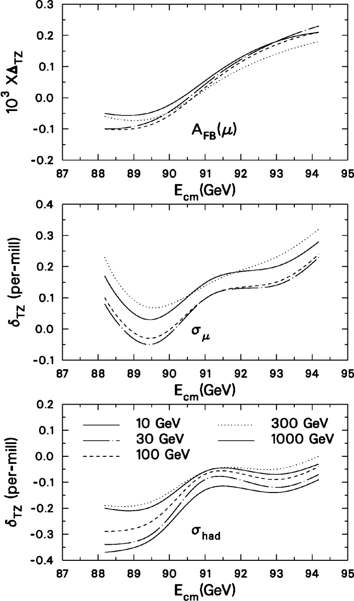
Figure 7: Relative deviations between TOPAZ0 and ZFITTER for hadronic cross-section in CA3 mode as a function of the Higgs boson mass. The curves correspond to a cut $s^{\prime}>0.01\,s$.

7 Initial-Final QED Interference

If initial-final QED (ISR-FSR) interference (IFI) is included in a calculation there is a conceptual problem with the meaning of the $s^{\prime}$-cut. In this case the definition of the variable $s^{\prime}$ is unnatural since one does no longer know the origin of the radiative photon (ISR or FSR). Only a cut on the invariant mass of the final-state $f\overline{f}$ system, $M(f\overline{f})$, makes sense.

There is another option: to select events with little initial-state radiation one can use a cut on the acollinearity angle $\theta_{\rm acol}$, between the outgoing fermion and anti-fermion. A cut on $\theta_{\rm acol}$ is roughly equivalent to a cut on the invariant mass of the $f\overline{f}$ system, indeed one may write

$$\frac{M^{2}}{s}\approx z_{\rm eff}={{1-\sin(\theta_{\rm acol}/2)}\over{1+\sin(\theta_{\rm acol}/2)}}\;,$$ (60)

therefore a cut of $\theta_{\rm acol}<10^{\circ}$ is roughly corresponding to the request that $M^{2}/s>0.84$.

The inclusion of initial-final QED interference in TOPAZ0 and in ZFITTER is done at ${\mathcal{O}}\left(\alpha\right)$, i.e., the ${\mathcal{O}}\left(\alpha\right)$ initial-final interference term is added linearly to the cross-sections without entering the convolution with ISR and without cross-talk to FSR. For loose cuts the induced uncertainty is rather small and the effect of the interference itself is minute, as shown below. On the contrary, when we select a tight acollinearity cut the resulting limit on the energy of the emitted photon becomes more stringent and the effect of interference grows. The corresponding theoretical uncertainty, due to missing higher-order corrections, is therefore expected to be larger.

A pragmatic point of view to improve upon the pure ${\mathcal{O}}\left(\alpha\right)$ inclusion of the interference, which however is not implemented in the codes, would be the following: let us consider corrections not belonging to the two classes of ISR and FSR. These non-factorizable corrections correspond to both interference terms and QED box diagrams. We have, therefore, three classes of contributions for the total cross-section: ISR, FSR and interference.

If we denote by $\sigma_{{}_{\rm K}}$ the sum of factorizable (Born) plus non-factorizable cross-sections the totally radiatively corrected process can be effectively described in terms of structure functions. In this case $s^{\prime}$ is still the square of the invariant mass available after initial-state QED radiation and $s^{\prime}\geq M^{2}(f\overline{f})\geq s_{0}$. Therefore we can write

$$\sigma(s)=\int_{z_{{}_{0}}}^{1}dzH_{\rm in}(z,s)\,H_{\rm fin}(z-z_{{}_{0}},{\hat{s}})\,{\hat{\sigma}}_{{}_{\rm K}}\bigl{(}{\hat{s}};M^{2}(f\overline{f})\geq s_{0}\bigr{)},$$ (61)

where $H_{\rm in,fin}$ is the initial- and final-state QED radiator and $z_{{}_{0}}=M^{2}(f\overline{f})/s$. Moreover ${\hat{\sigma}}_{{}_{\rm K}}$ is the kernel cross-section evaluated with the constraint $M^{2}(f\overline{f})\geq s_{0}$ and ${\hat{s}}=z\,s$. The accuracy obtainable with Eq.(61) depends on the various contributions included within the three factors, the initial-state radiator $H_{\rm in}$, the final-state radiator $H_{\rm fin}$ and the kernel cross-section including factorizable and non-factorizable parts.

7.1 Comparison for Extrapolated Setup

The effect of including or excluding initial-final state QED interference is shown in Tab.(32). As seen from the Table, the level of agreement between TOPAZ0 and ZFITTER does not deteriorate after the inclusion of initial-final state QED interference for loose $M^{2}$-cuts. For this setup the effect of ${\mathcal{O}}\left(\alpha\right)$ IFI is under control.

	Centre-of-mass energy in GeV
	$M_{{}_{Z}}-3$	$M_{{}_{Z}}-1.8$	$M_{{}_{Z}}$	$M_{{}_{Z}}+1.8$	$M_{{}_{Z}}+3$
No ISR/FSR interference, $s^{\prime}\geq 0.01\,s$
$\sigma_{\mu}\,$[nb]	0.22849	0.47657	1.48010	0.69512	0.40642
	0.22843	0.47653	1.47995	0.69509	0.40638
	+0.26	+0.08	+0.10	+0.04	+0.10
$\sigma_{\rm had}\,$[nb]	4.45012	9.59910	30.43639	14.18269	8.19892
	4.45146	9.60165	30.43824	14.18391	8.19923
	-0.30	-0.27	-0.06	-0.09	-0.04
$A^{\mu}_{{}_{\rm FB}}$	-0.28312	-0.16977	-0.00062	0.11186	0.15466
	-0.28330	-0.16985	-0.00066	0.11182	0.15461
	+0.18	+0.08	+0.04	+0.04	+0.05
No ISR/FSR interference, $s^{\prime}\geq M^{2}(\mu^{+}\mu^{-})\geq 0.01\,s$
$\sigma_{\mu}\,$[nb]	0.22840	0.47642	1.47967	0.69490	0.40628
	0.22836	0.47641	1.47962	0.69492	0.40627
	+0.18	+0.02	+0.03	-0.03	+0.02
$\sigma_{\rm had}\,$[nb]	4.44990	9.59865	30.43501	14.18203	8.19853
	4.45129	9.60132	30.43725	14.18342	8.19894
	-0.31	-0.29	-0.07	-0.10	-0.05
$A^{\mu}_{{}_{\rm FB}}$	-0.28321	-0.16981	-0.00062	0.11189	0.15470
	-0.28336	-0.16988	-0.00066	0.11184	0.15464
	+0.15	+0.07	+0.04	+0.05	+0.06
ISR/FSR interference, $s^{\prime}\geq M^{2}(\mu^{+}\mu^{-})\geq 0.01\,s$
$\sigma_{\mu}\,$[nb]	0.22783	0.47566	1.47970	0.69563	0.40684
	0.22779	0.47566	1.47967	0.69570	0.40686
	+0.18	0.0	+0.02	-0.10	-0.05
$\sigma_{\rm had}\,$[nb]	4.45083	9.59990	30.43495	14.18082	8.19761
	4.45221	9.60254	30.43717	14.18215	8.19797
	-0.31	-0.27	-0.07	-0.09	-0.04
$A^{\mu}_{{}_{\rm FB}}$	-0.28242	-0.16898	-0.00031	0.11177	0.15467
	-0.28287	-0.16934	-0.00031	0.11193	0.15473
	+0.45	+0.36	+0.00	-0.16	-0.06

Table 32: Effects of ISR/FSR QED interference for $\sigma_{\mu}$, $\sigma_{\rm had}$ and $A^{\mu}_{{}_{\rm FB}}$ (in CA3-mode). First row TOPAZ0, second row ZFITTER third row relative (absolute) deviations in per-mill. The scale $s$ is used for the running $\alpha$.

	Centre-of-mass energy in GeV
		$M_{{}_{Z}}-3$	$M_{{}_{Z}}-1.8$	$M_{{}_{Z}}$	$M_{{}_{Z}}+1.8$	$M_{{}_{Z}}+3$
$\sigma_{\mu}\,$[nb]	T	0.22311	0.47122	1.47473	0.68963	0.40076
		0.22153	0.46914	1.47464	0.69138	0.40204
		-7.13	-4.43	-0.06	+2.53	+3.18
	Z	0.22315	0.47127	1.47466	0.68967	0.40079
		0.22157	0.46922	1.47463	0.69148	0.40211
		-7.13	-4.37	-0.02	+2.62	+3.28
$A^{\mu}_{{}_{\rm FB}}$	T	-0.28347	-0.16849	0.00050	0.11539	0.16169
		-0.28074	-0.16613	0.00103	0.11425	0.16018
		+2.73	+2.36	+0.53	-1.14	-1.51
	Z	-0.28344	-0.16849	0.00047	0.11535	0.16166
		-0.28084	-0.16634	0.00104	0.11440	0.16025
		+2.60	+2.15	+0.57	-1.15	-1.41

Table 33: TOPAZ0/ZFITTER comparison of IFI effect for $M^{2}>0.8\,s$. First row is without IFI, second row is with IFI and third row is the net effect in per-mill. The scale $0$ is used for the running $\alpha$.

	Centre-of-mass energy in GeV
		$M_{{}_{Z}}-3$	$M_{{}_{Z}}-1.8$	$M_{{}_{Z}}$	$M_{{}_{Z}}+1.8$	$M_{{}_{Z}}+3$
$\sigma_{\mu}\,$[nb]	T	0.21932	0.46287	1.44794	0.67725	0.39366
		0.21775	0.46081	1.44785	0.67896	0.39492
		-7.21	-4.47	-0.06	+2.52	+3.19
$A^{\mu}_{{}_{\rm FB}}$	T	-0.28450	-0.16914	0.00033	0.11512	0.16106
		-0.28163	-0.16668	0.00087	0.11386	0.15937
		+2.87	+2.46	+0.54	-1.26	-1.69

Table 34: TOPAZ0 evaluation of IFI effect for $M^{2}(\mu^{+}\mu^{-})>13.83997\,$GeV and $\theta_{\rm acol}<10^{\circ}$. First row is without IFI, second row is with IFI and third row is the net effect in per-mill. The scale $0$ is used for the running $\alpha$.

We also perform other comparisons to understand the effect of IFI for various setups. First of all we use an extrapolated setup with a tight $M^{2}$-cut of $0.8\,s$ (it was $0.01\,s$ before). Note that such a cut is, not exactly, but approximately equivalent to $\theta_{\rm acol}=10^{\circ}$ (note that an $M^{2}$-cut takes into account only the isotropic part of the photon phase space). The result, reported in Tab.(34), shows that the two codes nicely agree for the net IFI effect also in case of tight $M^{2}$-cuts. Note that the effect of QED initial-final interference is quite sizeable, differently from what happens with loose cuts.

A further test, performed with TOPAZ0, selects another setup. Note that $E_{\rm th}=1\,$ GeV at $\sqrt{s}=M_{{}_{Z}}-3$ is equivalent to an $M^{2}$-cut of $M^{2}(\overline{f}f)\approx 2\,E_{\rm th}\sqrt{s}\approx 13.83997\,$GeV if we consider the radiative photon collinear with one of the final-state fermions. In this example we apply an $M^{2}$-cut as above and a cut of $10^{\circ}$ on the acollinearity so that the photon phase space is not isotropic anymore. The result is shown in Tab.(34).

The cut on acollinearity, superimposed on the $M^{2}$-cut, hardly changes the size of IFI effect, at least as seen by TOPAZ0. Roughly speaking, one computes IFI with a cut on $M^{2}$ simulated by the acollinearity and has to add a small portion of the photon phase space, subtracting, at the same time, the region not allowed by acol-cut. To understand which portion of photon phase-space is added we introduce variables

$$E_{+}=\frac{1}{2}\,\left(1-x_{1}+x_{2}\right)\,\sqrt{s}\;,\quad E_{-}=\frac{1}{2}\,x_{1}\,\sqrt{s}\;,\quad E_{\gamma}=\frac{1}{2}\,\left(1-x_{2}\right)\,\sqrt{s}\;.$$ (62)

and observe that this parametrisation has the advantage that in the limit where we neglect $m_{f}$ the boundaries of the phase space are of a triangular form

$$x_{1}=x_{2}\;,\\ x_{1}=1\cup x_{2}=0\;.$$ (63)

The boundary of the phase space corresponding to the selection criterion $\delta=\pi-\theta_{\rm ac}$ is, in the limit $m_{f}=0$, represented by

$$x^{2}_{1}-\left(1+x_{2}\right)\,x_{1}+{2\over{1+\cos\theta_{\rm ac}}}\,x_{2}=0.$$ (64)

Therefore, if we require some acollinearity cut and $M^{2}(\overline{f}f)\geq s_{0}$, the limits of integration are:

$$x^{\rm acol}_{2} \leq x_{2}\leq 1,\qquad x_{2}\leq x_{1}\leq 1,$$

$$\frac{s_{0}}{s}\leq x_{2}\leq x^{\rm acol}_{2},\qquad x_{2} \leq x_{1}\leq x^{-}_{1}\quad\cup\quad x^{+}_{1}\leq x_{1}\leq 1.$$ (65)

with

$$x^{\rm acol}_{2} = {{1-\sin(\theta_{\rm acol}/2)}\over{1+\sin(\theta_{\rm acol}/2)}},$$

$$x^{\pm}_{1} = \frac{1}{2}\,\Bigl{[}1+x_{2}\pm\sqrt{x^{2}_{2}+2\,\left(1-2\,\rho\right)\,x_{2}+1}\Bigr{]},$$

$$\rho = \frac{2}{1+\cos\theta_{\rm acol}}$$ (66)

$\sigma_{\rm had}\,$[nb]
	Centre-of-mass energy in GeV
	$M_{{}_{Z}}-3$	$M_{{}_{Z}}-1.8$	$M_{{}_{Z}}$	$M_{{}_{Z}}+1.8$	$M_{{}_{Z}}+3$
T	4.44990	9.59865	30.43501	14.18203	8.19853
$M^{2}\geq 0.01\,s$	4.45083	9.59990	30.43495	14.18082	8.19761
	+0.21	+0.13	-0.002	-0.09	-0.11
Z	4.45129	9.60132	30.43725	14.18342	8.19894
$M^{2}\geq 0.01\,s$	4.45221	9.60254	30.43717	14.18215	8.19797
	+0.21	+0.13	-0.003	-0.09	-0.12
T	4.36901	9.45847	30.05724	13.97471	8.05056
$M^{2}\geq 0.8\,s$	4.37172	9.46205	30.05739	13.97167	8.04831
$\alpha(s)$	+0.62	+0.38	+0.005	-0.22	-0.28
Z	4.36943	9.45848	30.04915	13.97099	8.04804
$M^{2}\geq 0.8\,s$	4.37214	9.46201	30.04923	13.96786	8.04573
$\alpha(s)$	+0.62	+0.37	+0.003	-0.22	-0.29
T	4.37186	9.46463	30.07686	13.98432	8.05646
$M^{2}\geq 0.8\,s$	4.37458	9.46821	30.07701	13.98127	8.05421
$\alpha(0)$	+0.62	+0.38	+0.005	-0.22	-0.28

Table 35: TOPAZ0/ZFITTER comparison of IFI inclusion for hadrons with $M^{2}$-cut. First entry is without IFI, second entry is with IFI, third entry is the IFI effect in per-mill. For the 0.8 cut there are two entries, corresponding to two different scales: $\alpha(s)$ and $\alpha(0)$.

The cut $M^{2}\geq 0.8\,s$ deserves a comment. For a fully extrapolated setup we know from a complete calculation [25] that the correct scale in the coupling is $s$, i.e., $\alpha(s)$. Therefore the two codes adopt the following scales: loose $M^{2}$ and $s^{\prime}$ cuts (up to $0.1s$) with $\alpha(s)$, tight cuts with $\alpha(0)$. Now, however, we are using a tight $M^{2}$-cut and there is an uncertainty, if one uses $\alpha(s)$ then partial higher corrections are seen, as expected. From Tab.(35) we see, however, that the net effect of IFI remains unchanged. The uncertainty associated with the choice of the scale, which becomes relevant only for high values of $s^{\prime}(M^{2})$-cuts, is common to all final states, including leptons.

Note that the T/Z agreement slightly deteriorates at such a tight cut (up to 0.3 per-mill at resonance). This is not at all surprising: for such tight cuts some common exponentiation of ISR and FSR is mandatory. On the contrary, one should conclude that the T/Z agreement remains remarkable even for very tight $M^{2}$ cuts.

In Tab.(36) we show the effect of changing the scale $\alpha(s)\to\alpha(0)$ in the muonic cross-section and asymmetry with $M^{2}$-cuts of $0.1\,s,0.5\,s$ and $0.8\,s$. The variations in cross-sections range from $\approx 0.03$ per-mill at $M^{2}=0.1\,s$ up to $\approx 4$ per-mill at $M^{2}=0.8\,s$. The effect of a scale change on the asymmetry is negligible.

For the hadronic cross-section at $M^{2}=0.8\,$ the variation induced by $\alpha(s)\to\alpha(0)$ is, at the peak, a $0.65$ per-mill to be compared with $3.75$ per-mill for muons; the sizeable difference is due to mass effects in QED FSR, $m_{\mu}\ll m_{q}$.

	Centre-of-mass energy in GeV
	$M_{{}_{Z}}-3$	$M_{{}_{Z}}-1.8$	$M_{{}_{Z}}$	$M_{{}_{Z}}+1.8$	$M_{{}_{Z}}+3$
$\sigma_{\mu}\,$[nb]
T $M^{2}\geq 0.1\,s\,\alpha(s)$	0.22615	0.47369	1.47484	0.69179	0.40382
T $M^{2}\geq 0.1\,s\,\alpha(0)$	0.22616	0.47370	1.47489	0.69182	0.40384
Diff.	0.04	0.02	0.03	0.04	0.05
T $M^{2}\geq 0.5\,s\,\alpha(s)$	0.22026	0.46327	1.44595	0.67712	0.39442
T $M^{2}\geq 0.5\,s\,\alpha(0)$	0.22051	0.46380	1.44762	0.67792	0.39490
Diff.	1.13	1.14	1.08	1.18	1.22
T $M^{2}\geq 0.8\,s\,\alpha(s)$	0.20926	0.44215	1.38382	0.64513	0.37335
T $M^{2}\geq 0.8\,s\,\alpha(0)$	0.21005	0.44381	1.38903	0.64769	0.37493
Diff.	3.76	3.74	3.75	3.95	4.21
$A^{\mu}_{{}_{\rm FB}}$
T $M^{2}\geq 0.1\,s\,\alpha(s)$	-0.28503	-0.16986	-0.00029	0.11224	0.15557
T $M^{2}\geq 0.1\,s\,\alpha(0)$	-0.28505	-0.16987	-0.00029	0.11225	0.15558
Diff.	0.02	0.01	0	-0.01	-0.01
T $M^{2}\geq 0.5\,s\,\alpha(s)$	-0.28603	-0.16981	0.00001	0.11312	0.15727
T $M^{2}\geq 0.5\,s\,\alpha(0)$	-0.28605	-0.16982	0.00001	0.11311	0.15726
Diff.	0.02	0.01	0	0.01	0.01
T $M^{2}\geq 0.8\,s\,\alpha(s)$	-0.28086	-0.16613	0.00130	0.11534	0.16236
T $M^{2}\geq 0.8\,s\,\alpha(0)$	-0.28091	-0.16616	0.00128	0.11530	0.16225
Diff.	0.05	0.03	0.02	0.04	0.09

Table 36: $\sigma_{\mu}$and $A^{\mu}_{{}_{\rm FB}}$, including IFI, for various $M^{2}$-cuts. First entry is with scale = $s$, second entry is with scale = $0$, third entry is the relative (absolute) difference in per-mill.

7.2 Comparison with Realistic Kinematical Cuts

Now we move to the classic setup, superimposing an acollinearity cut, a cut of 1 GeV on the energy of both outgoing fermions and a cut on the polar angular range of the outgoing fermion. The photon phase space is a little more complicated but not much. An acollinearity cut of $10^{\circ}$ or $25^{\circ}$ corresponds to $M^{2}=0.84\,s$ and $M^{2}=0.64\,s$, and is thus regarded as a tight cut. Therefore, the scale for $\alpha$ is $\alpha(0)$. The comparison is shown in Tabs.(37–40).

$\sigma_{\mu}\,$[nb] with $\theta_{\rm acol}<10^{\circ}$
	Centre-of-mass energy in GeV
$\theta_{\rm acc}$	$M_{{}_{Z}}-3$	$M_{{}_{Z}}-1.8$	$M_{{}_{Z}}$	$M_{{}_{Z}}+1.8$	$M_{{}_{Z}}+3$
T $0^{\circ}$	0.21932	0.46287	1.44795	0.67725	0.39366
	0.21776	0.46083	1.44785	0.67894	0.39491
	-7.16	-4.43	-0.07	+2.49	+3.17
Z $0^{\circ}$	0.21928	0.46285	1.44781	0.67722	0.39361
	0.21852	0.46186	1.44782	0.67814	0.39429
	-3.48	-2.14	+0.01	+1.36	+1.72
T $20^{\circ}$	0.19990	0.42207	1.32066	0.61759	0.35886
	0.19873	0.42049	1.32027	0.61873	0.35973
	-5.89	-3.76	-0.30	+1.84	+2.42
Z $20^{\circ}$	0.19987	0.42205	1.32053	0.61756	0.35881
	0.19892	0.42075	1.32021	0.61857	0.35959
	-4.78	-3.09	-0.24	+1.63	+2.17
T $40^{\circ}$	0.15034	0.31762	0.99428	0.46479	0.26989
	0.14979	0.31680	0.99360	0.46514	0.27021
	-3.67	-2.59	-0.68	+0.75	+1.18
Z $40^{\circ}$	0.15032	0.31760	0.99415	0.46474	0.26983
	0.14978	0.31680	0.99350	0.46511	0.27016
	-3.61	-2.53	-0.65	+0.80	+1.22

Table 37: TOPAZ0/ZFITTER comparison for the muonic cross-section of complete RO (CA3-mode) with the angular acceptance ($\theta_{\rm acc}=0,20,40^{\circ}$) and acollinearity ($\theta_{\rm acol}<10^{\circ}$) cuts. First row is without IFI, second row with IFI, third row is the relative (per-mill) effect of IFI.

$A^{\mu}_{{}_{\rm FB}}$ with $\theta_{\rm acol}<10^{\circ}$
	Centre-of-mass energy in GeV
$\theta_{\rm acc}$	$M_{{}_{Z}}-3$	$M_{{}_{Z}}-1.8$	$M_{{}_{Z}}$	$M_{{}_{Z}}+1.8$	$M_{{}_{Z}}+3$
T $0^{\circ}$	-0.28450	-0.16914	0.00033	0.11512	0.16107
	-0.28158	-0.16665	0.00088	0.11385	0.15936
	+2.92	+2.49	+0.55	-1.27	-1.71
Z $0^{\circ}$	-0.28453	-0.16911	0.00025	0.11486	0.16071
	-0.28282	-0.16783	0.00070	0.11475	0.16059
	+1.71	+1.28	+0.45	-0.11	-0.12
T $20^{\circ}$	-0.27509	-0.16352	0.00042	0.11171	0.15645
	-0.27259	-0.16146	0.00084	0.11064	0.15499
	+2.50	+2.06	+0.42	-1.07	-1.46
Z $20^{\circ}$	-0.27506	-0.16347	0.00035	0.11148	0.15616
	-0.27408	-0.16261	0.00070	0.11133	0.15594
	+0.98	+0.86	+0.35	-0.15	-0.22
T $40^{\circ}$	-0.24219	-0.14396	0.00054	0.09906	0.13903
	-0.24041	-0.14262	0.00078	0.09837	0.13809
	+1.78	+1.34	+0.24	-0.69	-0.94
Z $40^{\circ}$	-0.24207	-0.14386	0.00050	0.09893	0.13891
	-0.24151	-0.14343	0.00069	0.09890	0.13888
	+0.56	+0.43	+0.19	-0.03	-0.03

Table 38: TOPAZ0/ZFITTER comparison for the muonic forward-backward asymmetry of complete RO (CA3-mode) with the angular acceptance ($\theta_{\rm acc}=0,20,40^{\circ}$) and acollinearity ($\theta_{\rm acol}<10^{\circ}$) cuts. First row is without IFI, second row with IFI, third row is the absolute effect of IFI (per-mill).

$\sigma_{\mu}\,$[nb] with $\theta_{\rm acol}<25^{\circ}$
	Centre-of-mass energy in GeV
$\theta_{\rm acc}$	$M_{{}_{Z}}-3$	$M_{{}_{Z}}-1.8$	$M_{{}_{Z}}$	$M_{{}_{Z}}+1.8$	$M_{{}_{Z}}+3$
T $0^{\circ}$	0.22333	0.46971	1.46611	0.68690	0.40034
	0.22233	0.46838	1.46611	0.68812	0.40127
	-4.50	-2.84	0.00	+1.77	+2.32
Z $0^{\circ}$	0.22328	0.46968	1.46598	0.68688	0.40031
	0.22281	0.46905	1.46603	0.68754	0.40081
	-2.11	-1.34	+0.03	+0.96	+1.25
T $20^{\circ}$	0.20359	0.42835	1.33731	0.62648	0.36507
	0.20286	0.42733	1.33700	0.62725	0.36569
	-3.60	-2.39	-0.23	+1.23	+1.70
Z $20^{\circ}$	0.20357	0.42833	1.33718	0.62647	0.36505
	0.20321	0.42781	1.33689	0.62684	0.36536
	-1.77	-1.22	-0.22	+0.59	+0.85
T $40^{\circ}$	0.15320	0.32245	1.00698	0.47167	0.27479
	0.15286	0.32190	1.00635	0.47185	0.27500
	-2.22	-1.71	-0.63	+0.38	+0.76
Z $40^{\circ}$	0.15318	0.32243	1.00682	0.47164	0.27477
	0.15287	0.32192	1.00619	0.47180	0.27496
	-2.03	-1.58	-0.63	+0.34	+0.69

Table 39: TOPAZ0/ZFITTER comparison for the muonic cross-section of complete RO (CA3-mode) with the angular acceptance ($\theta_{\rm acc}=0,20,40^{\circ}$) and acollinearity ($\theta_{\rm acol}<25^{\circ}$) cuts. First row is without IFI, second row with IFI, third row is the relative (per-mill) effect of IFI.

$A^{\mu}_{{}_{\rm FB}}$ with $\theta_{\rm acol}<25^{\circ}$
	Centre-of-mass energy in GeV
$\theta_{\rm acc}$	$M_{{}_{Z}}-3$	$M_{{}_{Z}}-1.8$	$M_{{}_{Z}}$	$M_{{}_{Z}}+1.8$	$M_{{}_{Z}}+3$
T $0^{\circ}$	-0.28617	-0.17037	-0.00032	0.11324	0.15730
	-0.28501	-0.16923	0.00006	0.11293	0.15703
	+1.16	+1.14	+0.38	-0.31	-0.27
Z $0^{\circ}$	-0.28647	-0.17049	-0.00043	0.11293	0.15682
	-0.28555	-0.16975	-0.00005	0.11307	0.15701
	+0.92	+0.74	+0.48	+0.14	+0.19
T $20^{\circ}$	-0.27695	-0.16485	-0.00026	0.10974	0.15250
	-0.27611	-0.16404	0.00001	0.10955	0.15236
	+0.84	+0.81	+0.27	-0.19	-0.14
Z $20^{\circ}$	-0.27722	-0.16497	-0.00037	0.10944	0.15204
	-0.27657	-0.16447	-0.00009	0.10963	0.15229
	+0.65	+0.50	+0.28	+0.19	+0.25
T $40^{\circ}$	-0.24423	-0.14536	-0.00016	0.09703	0.13492
	-0.24381	-0.14501	-0.00004	0.09702	0.13500
	+0.42	+0.35	+0.12	-0.01	+0.08
Z $40^{\circ}$	-0.24445	-0.14545	-0.00026	0.09678	0.13454
	-0.24444	-0.14542	-0.00011	0.09700	0.13483
	+0.01	+0.03	+0.15	+0.22	+0.29

Table 40: TOPAZ0/ZFITTER comparison for the muonic forward-backward asymmetry of complete RO (CA3-mode) with the angular acceptance ($\theta_{\rm acc}=0,20,40^{\circ}$) and acollinearity ($\theta_{\rm acol}<25^{\circ}$) cuts. First row is without IFI, second row with IFI, third row is the absolute effect of IFI (per-mill).

There are several points to be discussed here. Although for the peak energy, we register generally a good agreement between TOPAZ0 4.4 and ZFITTER 5.20, the situation for the off-peak points is signalling a disagreement. Here TOPAZ0 4.4 confirms the same size of IFI effect of previous situations, while ZFITTER 5.20 sees half of the effect. This is a somewhat unique situation, the only one where TOPAZ0 4.4 and ZFITTER 5.20 register a substantial disagreement. This disagreement should not be taken as a measure of the real theoretical uncertainty.

Recent work of the Zeuthen group [40] has contributed substantially in understanding the origin of IFI-discrepancy, the IFI effect being so different in the two codes when realistic cuts are imposed. For the case of full angular acceptance, the work of [40] contains a full list of updated results. It recalculates photonic corrections with acollinearity cuts, having in mind applications to ZFITTER. The conclusions of this work are that after inclusion of the new calculation the agreement with TOPAZ0 4.4 is 0.1 per-mill (at the wings) or better (on resonance) for cross-sections. Work is in progress to update the inclusion of angular cuts. Thanks to the important contribution of the Zeuthen group, the IFI discrepancy with realistic cuts is on its way to be fully solved.

As stated above, the introduction of angular cuts will represent the next step in Zeuthen’s program. For the moment, therefore, we have at our disposal only the comparison between TOPAZ0 4.4 and ZFITTER 5.20. This section contains many IFI numbers based on these two programs, so that it should become clear under which conditions the discrepancies are large or small. Based on this the experiments will then have to derive an adequate solution for ROs with realistic cuts, concerning the magnitude of the effect and its theoretical uncertainty. Some possibilities are:

1. Use current IFI as implemented in TOPAZ0 4.4/ZFITTER 5.20 and assign overall uncertainty from the comparison,

2. Use ${\mathcal{O}}\left(\alpha\right)$ IFI of, e.g., KORALZ to remove IFI effects from the ROs and fit the ROs with TOPAZ0/ZFITTER having switched off IFI. Of course, in this case the KORALZ implementation of IFI must be evaluated to obtain the theory uncertainty.

3. Wait for an updated ZFITTER code and repeat the TOPAZ0/ZFITTER comparison to estimate the theoretical uncertainty.

7.3 Experimental Aspects of Initial-Final QED Interference

As a last remark we observe that also the treatment of initial-final QED interference effects by the experiments in arriving at quoted ROs has to be taken into account. For example, if the Monte Carlo generators used to correct for efficiency and to extrapolate for geometrical acceptance do not contain interference (as is the case, for example, in the current versions of JETSET/PYTHIA, or KORALZ used in multi-photon mode), then the extrapolated and quoted ROs somehow miss interference.

One main question is therefore: do QED interference effects enter only in the extrapolation step, e.g., $\cos(\theta)\to 1$? If so, then at least the fits are under control since the effect of missing IFI cancels out when TOPAZ0/ZFITTER are also run without interference. However, if interference effects already show up within the accepted region, then not only the quoted ROs are ill-defined but there are also problems in fitting them.

It is of course a matter of the size of the effect. From our study we can draw some conclusion, despite the present disagreement in case realistic cuts are imposed. If we stay at the $Z$-peak where our predictions show agreement we observe a $-0.07,-0.30,-0.68$ $(+0.01,$$-0.24,-0.65)$ per-mill effect in TOPAZ0 (ZFITTER) on the cross-section for $\theta_{\rm acol}<10^{\circ}$ and $\theta_{\rm acc}=0^{\circ},20^{\circ}$ and $40^{\circ}$. The effect of interference grows when reducing the angular acceptance from $0^{\circ}$ to $40^{\circ}$. At the wings the effect is becoming smaller for reduced angular acceptance, but the rate of decreasing is not fast; for TOPAZ0/ZFITTER the effect of IFI is still $-3.67/-3.61~{}(1.18/1.22)$ per-mill at $\theta_{\rm acc}=40^{\circ}$ and $\sqrt{s}=M_{{}_{Z}}-3~{}(+3)$. Note that around $\theta_{\rm acc}=40^{\circ}$ TOPAZ0 and ZFITTER start to agree well, so the previous statement is not affected by differences in the codes. For $\theta_{\rm acol}<25^{\circ}$ the effect at the peak goes from zero at $\theta_{\rm acc}=0^{\circ}$ to $-0.63$ per-mill at $\theta_{\rm acc}=40^{\circ}$. At the wings the effect is $-2$ per-mill and $+0.7$ per-mill respectively for $\theta_{\rm acc}=40^{\circ}$ (with good agreement between the codes). For asymmetries, the interference effect decreases in magnitude with reduced angular acceptance at and below the peak energy. This is also the case for TOPAZ0 above the peak, while a different behaviour is observed for ZFITTER.

Our conclusion is that the size of the IFI effect is at the level of few per-mill even within a fiducial volume cut. In order to minimise the effect we recommend to quote results, e.g., asymmetries, within a fiducial volume, at least at the wings of the $Z$ resonance.

8 Realistic Observables in the Model Independent Approach

As we have shown in Eq.(40) the main emphasis in the MI-approach is to organise the calculation of ROs in terms of POs for MI fits. One has to show the internal consistency of the procedure. First, one has to show that for POs with values as calculated in the SM, the ROs are by construction identical to the full SM RO calculation. Next one has to make sure that the ROs computed by different codes also agree for MI calculations when the POs do not have SM values, but are varied over a range of PO values corresponding to at least the current experimental errors on POs for a single experiment.

It is one of the main goals of our study to perform such comparison with TOPAZ0 and ZFITTER. Of course it will not be possible to present here the full comparison for arbitrary ROs but we will compare few significant examples, e.g., few ROs like $\sigma_{\mu},\sigma_{{h}}$ and $A^{\mu}_{{}_{\rm FB}}$, at fixed $M_{{}_{Z}},m_{t},M_{{}_{H}},$ $\alpha(M^{2}_{{}_{Z}}),\alpha_{{}_{S}}(M^{2}_{{}_{Z}})$, as a function of $\Gamma_{{}_{Z}},\sigma^{0}_{{h}},R_{l}$ and $A^{0,\rm l}_{{}_{\rm FB}}$. Note that we do not vary $M_{{}_{Z}}$, both because its experimental error is so small and because it is also a SM parameter. We vary the remaining POs, one by one. Assuming the experimental errors to be twice the current LEP errors [13], we obtain:

$$\Gamma_{{}_{Z}} = 2.4958\pm 0.0048\,\;\mathrm{GeV},$$

$$\sigma^{0}_{{h}} = 41.473\pm 0.116\,\;\mathrm{nb},$$

$$R_{l} = 20.748\pm 0.052,$$

$$A^{0,\rm l}_{{}_{\rm FB}} = 0.01613\pm 0.00192\,.$$ (67)

We vary the POs by twice their experimental errors. The corresponding deviations between the two codes will give an estimate of the technical precision of the procedure. For the SM initialisation, our preferred setup of SM input parameters is used. The effects of IFI and ISPP are not included.

We show the MI comparisons in Figs. 8–15. The solid curve gives deviations corresponding to the current experimental value of the relative PO, the dotted (dashed) curve corresponds to PO$\,\pm\,2\,\times$ the experimental errors listed in Eq.(67). For some of the figures the three curves become indistinguishable, typically the hadronic cross section has a constant deviation between the two MI-calculations if we vary $R_{l}$ or $A^{0,l}_{{}_{\rm FB}}$.

From Fig. 8 to Fig. 11 we use an extrapolated setup with an $s^{\prime}$-cut of $0.01\,s$ and report the relative (in per-mill) TOPAZ0-ZFITTER deviations for $\sigma_{\mu},\sigma_{{h}}$ and the absolute deviations for $A^{\mu}_{{}_{\rm FB}}$. In Figs. 12–15 we show similar comparisons for the muonic ROs with realistic cuts. We choose $20^{\circ}<\theta_{-}<160^{\circ}$, $\theta_{\rm acoll}<10^{\circ}$, and $E_{th}(\mu^{\pm})=1\,$GeV. There is no appreciable difference in behaviour with respect to the $s^{\prime}$ case shown before.

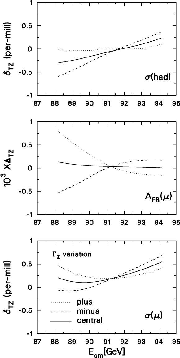
Figure 8: Relative deviations between TOPAZ0 and ZFITTER for muonic and hadronic cross-section and absolute deviations for muonic forward-backward asymmetry in CA3 mode and for $s^{\prime}>0.01\,s$. The solid curve gives deviations corresponding to the current experimental value of $\Gamma_{{}_{Z}}$, the dotted (dashed) curve corresponds to PO$\,\pm\,2\,\times$ the experimental error.

Figure 9: Relative deviations between TOPAZ0 and ZFITTER for muonic and hadronic cross-section and absolute deviations for muonic forward-backward asymmetry in CA3 mode and for $s^{\prime}>0.01\,s$. The solid curve gives deviations corresponding to the current experimental value of $\sigma^{0}_{\rm had}$, the dotted (dashed) curve corresponds to PO$\,\pm\,2\,\times$ the experimental error.

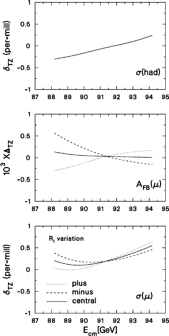
Figure 10: Relative deviations between TOPAZ0 and ZFITTER for muonic and hadronic cross-section and absolute deviations for muonic forward-backward asymmetry in CA3 mode and for $s^{\prime}>0.01\,s$. The solid curve gives deviations corresponding to the current experimental value of $R_{l}$, the dotted (dashed) curve corresponds to PO$\,\pm\,2\,\times$ the experimental error.

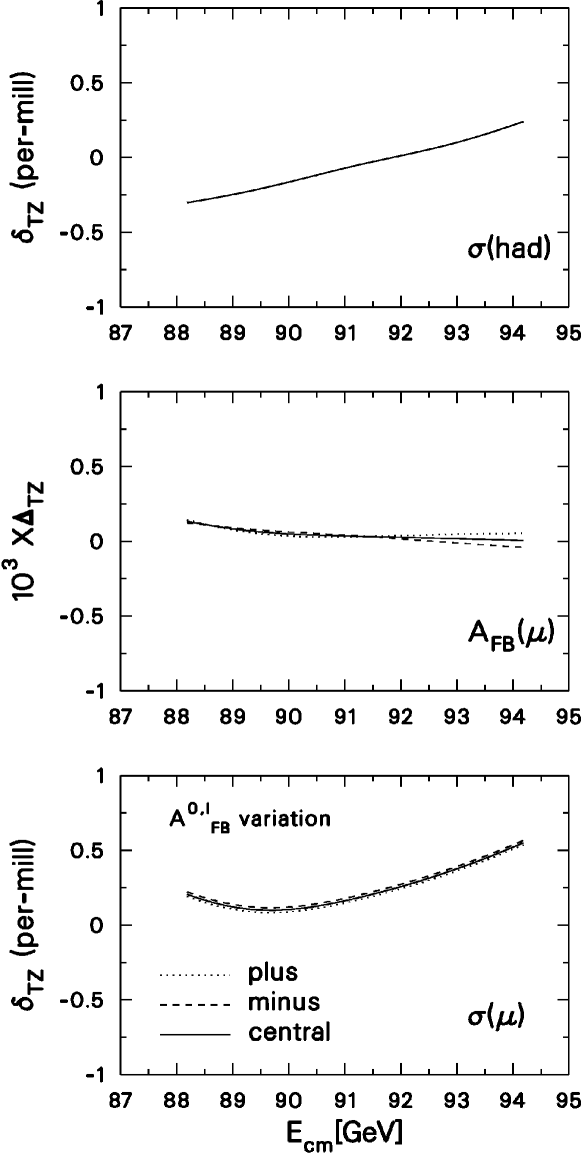
Figure 11: Relative deviations between TOPAZ0 and ZFITTER for muonic and hadronic cross-section and absolute deviations for muonic forward-backward asymmetry in CA3 mode and for $s^{\prime}>0.01\,s$. The solid curve gives deviations corresponding to the current experimental value of $A^{0,l}_{{}_{\rm FB}}$, the dotted (dashed) curve corresponds to PO$\,\pm\,2\,\times$ the experimental error.

Figure 12: Relative deviations between TOPAZ0 and ZFITTER for muonic cross-section and absolute deviations for muonic forward-backward asymmetry in CA3 mode and for realistic cuts. The solid curve gives deviations corresponding to the current experimental value of $\Gamma_{{}_{Z}}$, the dotted (dashed) curve corresponds to PO$\,\pm\,2\,\times$ the experimental error.

Figure 13: Relative deviations between TOPAZ0 and ZFITTER for muonic cross-section and absolute deviations for muonic forward-backward asymmetry in CA3 mode and for realistic cuts. The solid curve gives deviations corresponding to the current experimental value of $\sigma^{0}_{\rm had}$, the dotted (dashed) curve corresponds to PO$\,\pm\,2\,\times$ the experimental error.

Figure 14: Relative deviations between TOPAZ0 and ZFITTER for muonic cross-section and absolute deviations for muonic forward-backward asymmetry in CA3 mode and for realistic cuts. The solid curve gives deviations corresponding to the current experimental value of $R_{l}$, the dotted (dashed) curve corresponds to PO$\,\pm\,2\,\times$ the experimental error.

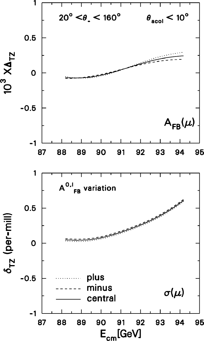
Figure 15: Relative deviations between TOPAZ0 and ZFITTER for muonic cross-section and absolute deviations for muonic forward-backward asymmetry in CA3 mode and for realistic cuts. The solid curve gives deviations corresponding to the current experimental value of $A^{0,l}_{{}_{\rm FB}}$, the dotted (dashed) curve corresponds to PO$\,\pm\,2\,\times$ the experimental error.

Most of the plots in Figs. 8–15 show a crossing of the three curves (central, plus and minus) at $s=M^{2}_{{}_{Z}}$. This means that at the $Z$-pole the MI implementations of the two code are fully equivalent while the MI treatment of the off-resonance terms is somewhat different. This fact is largely expected since MI-implementations or the MI-SM splitting is far from unique. However, the rather satisfactory level of agreement is telling us that the associated theoretical uncertainty in extracting POs from ROs is not substantially different or badly deteriorated with respect to the one that we have shown in SM comparisons.

Another typical effect is that TOPAZ0 ROs tend to be lower than ZFITTER ROs at PO$\,-\,2\,\times\,$ experimental error and on the low-energy side of the resonance. With increasing energy the curves tend to cross at the $Z$-peak and to reverse their sign on the high energy side. On the contrary, for PO$\,+\,2\,\times\,$ experimental error, TOPAZ0 is higher below the resonance and lower above it.

In Fig. 16 we compare TOPAZ0 and ZFITTER predictions by computing $\sigma_{\mu},\sigma_{{h}}$ and $A^{\mu}_{{}_{\rm FB}}$ with and $s^{\prime}$-cut of $0.01\,s$. The solid line gives deviations in the SM predictions initialised with our preferred setup. The dotted line gives deviations from the two MI predictions in case the ROs are computed in term of POs evaluated at their (code dependent) SM values. From comparing the two sets of curves we see that no serious degradation arises in the transition RO(SM,T,Z) $\,\to\,$ RO(PO${}_{\rm SM},{\tt T,Z}$). In particular we continue to register a very good agreement around the peak.

From these figures it emerges that, compared to the SM comparison, the agreement is still reasonable. Much more interesting than the deviations shown here would be to compare differences between MI fits performed with TOPAZ0 and ZFITTER using the same RO data set, clearly a task to be done by the experimental collaborations. The differences shown in the figures will cause differences in MI-fit results between TOPAZ0 and ZFITTER for the same input set of ROs. However, the effects have to be seen compared to the fit (experimental) errors. Approximately, the differences in ROs seen at the pole centre-of-mass energy will be those observed in the corresponding POs.

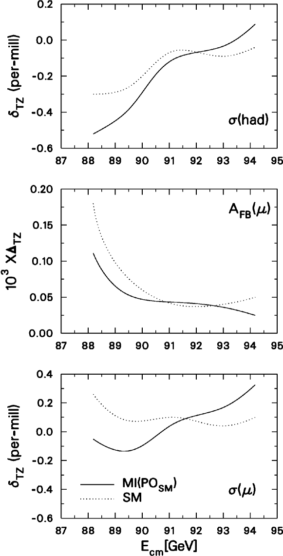
Figure 16: Relative deviations between TOPAZ0 and ZFITTER for muonic and hadronic cross-section and absolute deviations for muonic forward-backward asymmetry in CA3 mode and for $s^{\prime}>0.01\,s$. The solid curve gives deviations corresponding to SM predictions, the dotted curve corresponds to a MI prediction where PO are initialised to their SM values.

9 Theoretical Uncertainties for Realistic Observables

When varying options in the calculation of ROs based on POs or SM parameters, the theoretical uncertainties on ROs are obtained. This is discussed in the following. However, when the experimental collaborations analyse their measurements of ROs, this procedure is inverted by fitting POs or SM parameters to the measured ROs: Varying options, the changes in fitted parameters reflect the theoretical uncertainties associated with the calculation of ROs. This way the theoretical uncertainties on ROs are propagated back to the fitted parameters. Care must be taken not to double-count theoretical uncertainties in the SM calculation of POs which propagate to ROs, when SM parameters are determined in a fit to POs themselves determined in a MI fit to ROs.

9.1 Uncertainties in Standard Model Calculations

We now propagate the various electroweak options in SM calculations from $\mathrm{PO=PO(SM)}$ to $\mathrm{RO=RO(SM)}$. These options are described in Section 3.4 and are those used in describing the theoretical uncertainties at the level of PO. In addition there are other uncertainties, which we have already discussed, like those associated to different treatments of initial-state QED radiation. The corresponding flag values in TOPAZ0/ZFITTER are discussed in the following.

In TOPAZ0 the flag OHC=’Y’ selects next-to-leading and higher-order hard-photon contributions. Therefore this flag should not be varied. Once OHC=’Y’ is initialised TOPAZ0’s flag ORAD will select the type of next-to-leading and higher-order hard-photon contributions to be included, (A,D,E,F,Y). F [34] is the recommended choice; Y [35] has been implemented after version 4.3 and uses the order $\alpha^{3}$ YFS radiator. The other choices, A,D,E, remain for compatibility tests with previous versions and are not to be included in the estimate of the theoretical uncertainty. OFS=’D’,’Z’ selects the treatment of higher-order final-state QED corrections, see below. For the remaining TOPAZ0’s flags we observe the following. With OWBOX weak boxes are included ’Y’ or not ’N’. The correct choice is always ’Y’. At the $Z$-resonance, but only there, weak boxes can be neglected having a relative contribution $\leq 10^{-4}$. To give an example, for the muonic cross-section the effect of weak boxes is $-0.01$ per-mill at $\sqrt{s}=M_{{}_{Z}}$ and $+0.17~{}(-0.15)$ per-mill at the left (right) wing. Flags OAAS, OWEAK must be kept equal to ’N’, ’R’, respectively.

In ZFITTER, the flag FOT2 controls which radiator is used for inital-state QED radiation, FOT2=-1,0,1,2,3,4,5. Values FOT2=3,5 switch between the additive (default) and the factorized order $\alpha^{3}$ radiator, respectively. The remaining FOT2 flag values are kept for compatibility tests with previous versions and are not to be included in the estimate of the theoretical uncertainty. Weak boxes are switched off/on with the flag BOXD=0,1, respectively, and must always be on. The flag CONV controls the convolution of electroweak couplings and is discussed in Section 6. This flag must be kept fixed at a value larger than zero.

For the muonic and hadronic cross-sections and for the muonic forward-backward asymmetry we find the results reported in Tab.(41). These results are obtained by running TOPAZ0 under different options. As for POs, we show the central value for ROs evaluated at the preferred setup; the minus error for $\mbox{RO}_{\it central}-\min_{\rm opt}\,\mbox{RO}$ and the plus error for $\max_{\rm opt}\,\mbox{RO}-\mbox{RO}_{\it central}$. For cross-section the errors are reported in pb and, when available, we also show the absolute differences T-Z. From Tab.(41) we observe that the difference between TOPAZ0 and ZFITTER RO is fully compatible with the TOPAZ0-estimated theoretical uncertainty.

$\sqrt{s}\,$[GeV]	central	minus error	plus error	T-Z
$\sigma_{\mu}$
$M_{{}_{Z}}-3$	$0.22849\,\;\mathrm{nb}$	$0.04\,\;\mathrm{pb}$	$\leq 0.01\,\;\mathrm{pb}$	$0.07\,\;\mathrm{pb}$
$M_{{}_{Z}}-1.8$	$0.47657\,\;\mathrm{nb}$	$0.08\,\;\mathrm{pb}$	$0.01\,\;\mathrm{pb}$	$0.04\,\;\mathrm{pb}$
$M_{{}_{Z}}$	$1.48010\,\;\mathrm{nb}$	$0.09\,\;\mathrm{pb}$	$0.20\,\;\mathrm{pb}$	$0.16\,\;\mathrm{pb}$
$M_{{}_{Z}}+1.8$	$0.69512\,\;\mathrm{nb}$	$0.08\,\;\mathrm{pb}$	$0.06\,\;\mathrm{pb}$	$0.03\,\;\mathrm{pb}$
$M_{{}_{Z}}+3$	$0.40642\,\;\mathrm{nb}$	$0.06\,\;\mathrm{pb}$	$0.03\,\;\mathrm{pb}$	$0.04\,\;\mathrm{pb}$
$A^{\mu}_{{}_{\rm FB}}$
$M_{{}_{Z}}-3$	$-0.28312$	$0.00009$	$0.00001$	0.00018
$M_{{}_{Z}}-1.8$	$-0.16977$	$0.00008$	$0.00004$	0.00008
$M_{{}_{Z}}$	$-0.00062$	$0.00006$	$0.00009$	0.00004
$M_{{}_{Z}}+1.8$	$0.11186$	$0.00004$	$0.00012$	0.00004
$M_{{}_{Z}}+3$	$0.15466$	$0.00004$	$0.00012$	0.00005
$\sigma^{\mu}_{{}_{\rm F}}$
$M_{{}_{Z}}-3$	$0.08190\,\;\mathrm{nb}$	$0.03\,\;\mathrm{pb}$	$\leq 0.01\,\;\mathrm{pb}$
$M_{{}_{Z}}-1.8$	$0.19783\,\;\mathrm{nb}$	$0.05\,\;\mathrm{pb}$	$0.01\,\;\mathrm{pb}$
$M_{{}_{Z}}$	$0.73959\,\;\mathrm{nb}$	$0.04\,\;\mathrm{pb}$	$0.17\,\;\mathrm{pb}$
$M_{{}_{Z}}+1.8$	$0.38644\,\;\mathrm{nb}$	$0.06\,\;\mathrm{pb}$	$0.08\,\;\mathrm{pb}$
$M_{{}_{Z}}+3$	$0.23464\,\;\mathrm{nb}$	$0.04\,\;\mathrm{pb}$	$0.04\,\;\mathrm{pb}$
$\sigma^{\mu}_{{}_{\rm B}}$
$M_{{}_{Z}}-3$	$0.14659\,\;\mathrm{nb}$	$0.02\,\;\mathrm{pb}$	$\leq 0.01\,\;\mathrm{pb}$
$M_{{}_{Z}}-1.8$	$0.27874\,\;\mathrm{nb}$	$0.03\,\;\mathrm{pb}$	$\leq 0.01\,\;\mathrm{pb}$
$M_{{}_{Z}}$	$0.74051\,\;\mathrm{nb}$	$0.04\,\;\mathrm{pb}$	$0.04\,\;\mathrm{pb}$
$M_{{}_{Z}}+1.8$	$0.30868\,\;\mathrm{nb}$	$0.02\,\;\mathrm{pb}$	$\leq 0.01\,\;\mathrm{pb}$
$M_{{}_{Z}}+3$	$0.17178\,\;\mathrm{nb}$	$0.02\,\;\mathrm{pb}$	$\leq 0.01\,\;\mathrm{pb}$
$\sigma_{\rm had}$
$M_{{}_{Z}}-3$	$4.45012\,\;\mathrm{nb}$	$0.99\,\;\mathrm{pb}$	$1.40\,\;\mathrm{pb}$	$-1.29\,\;\mathrm{pb}$
$M_{{}_{Z}}-1.8$	$9.59909\,\;\mathrm{nb}$	$1.81\,\;\mathrm{pb}$	$3.41\,\;\mathrm{pb}$	$-2.49\,\;\mathrm{pb}$
$M_{{}_{Z}}$	$30.43639\,\;\mathrm{nb}$	$1.85\,\;\mathrm{pb}$	$14.27\,\;\mathrm{pb}$	$-11.83\,\;\mathrm{pb}$
$M_{{}_{Z}}+1.8$	$14.18269\,\;\mathrm{nb}$	$2.14\,\;\mathrm{pb}$	$6.01\,\;\mathrm{pb}$	$-1.27\,\;\mathrm{pb}$
$M_{{}_{Z}}+3$	$8.19892\,\;\mathrm{nb}$	$1.46\,\;\mathrm{pb}$	$3.38\,\;\mathrm{pb}$	$-0.36\,\;\mathrm{pb}$

Table 41: Theoretical uncertainties for $\sigma_{\mu},A^{\mu}_{{}_{\rm FB}},\sigma^{\mu}_{{}_{\rm F,B}}$ and for $\sigma_{\rm had}$ from TOPAZ0.

Finally we illustrate the effect of different treatments of final-state QED radiation in the presence of severe kinematical cuts. A possible source of theoretical uncertainty can be introduced when cuts are present, due to a different treatment of higher-order final-state QED effects: it can lead to differences which in general depend on the experimental cuts required and that may grow for particularly severe cuts. It was already shown [1] that two possible prescriptions,

• completely factorized final-state QED correction versus

• factorized leading-terms and non-leading contributions summed up,

can lead to substantial differences. In TOPAZ0 the flag OFS selects the treatment of higher-order final-state QED corrections; (D) or (Z), respectively. In ZFITTER, the first option, completely factorized final-state QED correction, is implemented. TOPAZ0 predicts for $\sigma^{\mu}$ and $20^{\circ}<\theta_{-}<120^{\circ},E_{\rm th}>15\,$GeV, $\theta_{\rm acol}<10^{\circ}$ an uncertainty of 1.2 per-mill at the five energy points. On the contrary for a loose cut of $E_{\rm th}>1\,$GeV we obtain a reduction to a mere 0.1 per-mill.

9.2 Uncertainties in Model Independent Calculations

Having discussed the theoretical uncertainties associated with the SM calculations of ROs, we also need to address the question of uncertainties for the MI-calculations, $\mathrm{RO=RO(PO)}$. The result is that one has all errors already quoted for RO(SM), Tab.(41), $\,\oplus\,$ those derived from varying PO away from their SM values and obtained by comparing TOPAZ0 with ZFITTER, Figs. 8–15.

Note that in the SM there are relations like ${\rm PO}_{1}=f({\rm PO}_{2})=F(M_{{}_{Z}},m_{t},\dots)$. With PO = PO(SM) one has to make sure that, no matter how the MI-structure is built, MI(T) must be equal to MI(Z). But when we break the SM-relations then several possibilities arise: one may write everywhere PO₁ or $f({\rm PO}_{2})$ and the difference is a measure of the associated uncertainty.

Alternatively one can estimate this uncertainties internally to each code by running in MI mode with all the relevant electroweak and QED flag variations as discussed before. The structure of the MI calculations is such that, given the decomposition PO $\,\oplus\,$ SM remnant, electroweak flag changing will effect the latter (the SM complement) and leave unaltered the PO (MI) component. To give an example, the whole $Z-\gamma$ interference in the quark sector is taken from the SM remnant and, therefore, influenced by flag setting.

10 Production of Secondary Pairs

Finally we come to the inclusion of pair-production in the calculation of realistic observables. Radiative photons from the initial- or final-state fermions may convert, leading to additional (soft) $f\overline{f}$ pairs besides the primary pair. This leads to the problem of the signal definition, i.e., what is considered as (radiative correction to) fermion-pair production, and what is considered as genuine four-fermion production.

Note that most Monte Carlo event generators used for fermion pair production do not include the radiative production of secondary pairs. In case of final-state pair production, visible in the detector, this may bias efficiency and acceptance calculations, in particular if the primary pair is a lepton pair.

10.1 Initial-State Pair Production

A fermionic pair of four-momentum $q^{2}$ radiated from the $e^{+}$ or $e^{-}$ line gives a correction which is computed in [41]. Also for this term there are different treatments, i.e., we can exponentiate the pair-production according to the YFS formalism [42] or the same pairs can be included at ${\mathcal{O}}\left(\alpha^{2}\right)$. The physical uncertainty on the pair correction is given by that on the contribution of light-quark pairs, and is estimated to be $1.8\cdot 10^{-4}$ for cross-sections [42].

Both TOPAZ0 and ZFITTER adopt a hybrid solution which gives a remarkable agreement around the peak with the results of [42]. ZFITTER includes the radiation of $e,\mu,\tau$-pairs and hadronic pairs. TOPAZ0 does not include radiation of $\tau$-pairs, their contribution is below the accuracy requirement of ${\mathcal{O}}\left(10^{-4}\right)$. For technical details we refer to [4] since no further upgrading has been performed in the area of pair production.

A cut was selected so that $z_{\rm min}s=s^{\prime}=M^{2}(f\overline{f})>0.25\,s$, where $f\overline{f}$ denotes the primary pair, i.e., $z_{\rm min}$ is the minimum fraction of squared invariant mass of the final state (primary pair) after radiation of the additional initial-state pair (secondary pair). Since we neglect terms coming from ISPP $\,\otimes\,$ FSR there will be no difference between $s^{\prime}$-cuts and $M^{2}$-cuts as far as ISPP corrections are concerned. The soft-hard separator $\Delta$ has been fixed in the region where we see a plateau of stability.

The effect of including leptonic as well as hadronic pairs radiated from the initial state is summarised in Tab.(42). From Tab.(42) we observe that the inclusion of initial-state pair-production lowers the cross-sections up to an energy of $M_{{}_{Z}}+3$ where the effect becomes positive. At the peak pair production modifies $\sigma_{\mu}$ by $-2.55~{}(-2.53)$ per-mill according to TOPAZ0 (ZFITTER) and $\sigma_{\rm had}$ by -2.55 per-mill for both codes.

	Centre-of-mass energy in GeV
	$M_{{}_{Z}}-3$	$M_{{}_{Z}}-1.8$	$M_{{}_{Z}}$	$M_{{}_{Z}}+1.8$	$M_{{}_{Z}}+3$
$\sigma_{\mu}$
T	0.22849	0.47657	1.48010	0.69512	0.40642
	0.22796	0.47534	1.47633	0.69480	0.40713
	-2.32	-2.58	-2.55	-0.46	1.75
Z	0.22843	0.47653	1.47995	0.69509	0.40638
	0.22790	0.47532	1.47621	0.69478	0.40708
	-2.33	-2.55	-2.53	-0.45	1.73
$A^{\mu}_{{}_{\rm FB}}$
T	-0.28312	-0.16977	-0.00062	0.11186	0.15466
	-0.28377	-0.17020	-0.00062	0.11192	0.15439
	-0.65	-0.43	0.00	+0.06	-0.27
Z	-0.28330	-0.16985	-0.00066	0.11182	0.15461
	-0.28395	-0.17028	-0.00066	0.11187	0.15434
	-0.65	-0.43	0.00	+0.05	-0.27
$\sigma_{\rm had}$
T	4.45012	9.59910	30.43639	14.18269	8.19892
	4.43937	9.57410	30.35866	14.17587	8.21336
	-2.42	-2.60	-2.55	-0.48	1.76
Z	4.45146	9.60165	30.43824	14.18391	8.19923
	4.44070	9.57659	30.36069	14.17709	8.21345
	-2.42	-2.62	-2.55	-0.48	1.73

Table 42: The effect of including initial state pair production in TOPAZ0 and ZFITTER in CA3-mode, $s^{\prime}>0.01\,s$. First (fourth) entry is without, second (fifth) entry is with pair production. Third (sixth) entry is the net effect in per-mill of the inclusion.

10.2 Final-State Pair Production

The current versions of TOPAZ0 (4.4) and ZFITTER (5.20) do not include effects of final-state pair production. However, virtual and real corrections due to final-state pair production cancel to a large extent and the remaining effect is mostly absorbed in the running electromagnetic coupling $\alpha(s)$ entering the correction factor for FSR [43]. Therefore, the experimental event selections should not discriminate against additional (soft) pairs. Otherwise, a correction has to be applied before TOPAZ0/ZFITTER calculations can be compared with the measurements.

11 Conclusions

In Tab.(41) we show an estimate of the theoretical error for realistic observables as computed internally by TOPAZ0. Another piece of information is given by the differences TOPAZ0 - ZFITTER among the (theoretical) central values for each quantity: these differences are basically (even though not totally) a measure of the effect induced by a variation in the renormalization scheme.

Consider, however, the complete hadronic cross-section (in CA3 $s^{\prime}$-mode): the differences (in per-mill) are $-0.30,-0.27,-0.06,-0.09,-0.04$ for the five centre-of-mass energies. There are two different origins for them, differences already present in the de-convoluted cross-sections (SD-mode) and differences due to convolution with initial-state QED radiation. For the former we find (in per-mill)

$$-0.38,\;-0.30,\;-0.07,\;-0.15,\;-0.14.$$ (68)

The effect of convolution is found to be (in per-mill)

$$+0.06,\;+0.02,\;+0.01,\;+0.07,\;+0.14.$$ (69)

Especially on the high-energy side of the resonance we observe a partial compensation, leading to a small overall uncertainty. A more conservative attitude consists in adopting some rough approximation thus defining

$$\sigma(s)=\sigma^{\rm SD}\,\left(1+\delta^{\rm dec}\right),$$ (70)

and adding the errors in quadrature:

$$\Delta\sigma = \sigma^{\rm{T}}-\sigma^{\rm{Z}},\quad\Delta\sigma^{\rm SD}=\sigma^{\rm{SD,T}}-\sigma^{\rm{SD,Z}},$$

$$\left(\Delta\delta^{\rm dec}\right)^{2} = \biggl{[}\frac{\Delta\sigma}{\sigma^{\rm SD}}\biggr{]}^{2}+\biggl{[}\frac{\sigma\Delta\sigma^{\rm SD}}{\left(\sigma^{\rm SD}\right)^{2}}\biggr{]}^{2}.$$ (71)

In this way we end up with an estimate of the theoretical error of

$$2.73\,\;\mathrm{pb},\;4.76\,\;\mathrm{pb},\;3.51\,\;\mathrm{pb},\;3.23\,\;\mathrm{pb},\;1.71\,\;\mathrm{pb},\quad\mbox{or}$$

$$0.061\%,\;\;0.050\%,\;\;0.012\%,\;\;0.023\%,\;\;0.021\%,$$ (72)

for the complete hadronic cross-section. Although quite conservative, we consider the above as a safe estimate of the theoretical error. A comparison with the results of Tab.(41) shows a substantial agreement with the estimate made internally by TOPAZ0. For the complete muonic cross-section we find

$$0.07\,\;\mathrm{pb},\;0.06\,\;\mathrm{pb},\;0.19\,\;\mathrm{pb},\;0.11\,\;\mathrm{pb},\;0.08\,\;\mathrm{pb}\quad\mbox{or}$$

$$0.030\%,\;\;0.014\%,\;\;0.013\%,\;\;0.016\%,\;\;0.021\%.$$ (73)

In both cases, the uncertainty arising due to the uncertainty on the ISPP contribution has to be added.

For the muonic forward-backward asymmetry we find results which are practically indistinguishable from those already reported in Tab.(41).

12 Acknowledgements

The present documentation is the result of an intensive collaboration with the experimentalists of the LEP electroweak working group. We are obliged to all of them for many fruitful discussions. We are particularly thankful to T. Kawamoto, A. Olshevski and G. Quast. We would like to express deep thanks to physicists who joined the TOPAZ0 and ZFITTER teams in course of many years: G. Montagna, O. Nicrosini, F. Piccinini, and R. Pittau and M. Bilenky, A. Chizhov, P. Christova, M. Jack, L. Kalinovskaya, A. Olshevski, S. Riemann, T. Riemann, M. Sachwitz, A. Sazonov, Yu. Sedykh, and I. Sheer. Without their contributions the two programs would not be what they are.

References

-
[1]
G. Montagna, O. Nicrosini, G. Passarino,
F. Piccinini and R. Pittau, Comput. Phys. Commun. 76 (1993) 328;
G. Montagna, O. Nicrosini, G. Passarino and F. Piccinini, Comput. Phys. Commun. 93 (1996) 120;
G. Montagna, O. Nicrosini, G. Passarino and F. Piccinini, hep-ph/9804211. - [2] D. Bardin et al., Nucl. Phys. B351 (1991) 1; Z. Phys. C44 (1989) 493; Phys. Lett. B255 (1991) 290; CERN-TH.6443/1992, May 1992; hep-ph/9412201.
- [3] Physics at LEP1, G. Altarelli, R. Kleiss and C. Verzegnassi eds., CERN-89-08, Vol.1 (1989)
- [4] D. Bardin et al. Electroweak Working Group Report, in Reports of the Working Group on Precision Calculations for the Resonance, D. Bardin, W. Hollik and G. Passarino eds., CERN-95-03, p. 7.
- [5] D. Bardin and G. Passarino, Upgrading of Precision Calculations for Electroweak Observables, hep-ph/9803425.
-
[6]
The FORTRAN source code of TOPAZ0
version 4.4 is available at:
http://www.to.infn.it/~giampier/topaz0.html on the world-wide web. -
[7]
The FORTRAN source code of ZFITTER
version 5.20 is available at:
http://www.ifh.de/~riemann/Zfitter/zf.html on the world-wide web and at: /afs/cern.ch/user/b/bardindy/public/ZF5_20/. - [8] C. Caso et al., The 1998 Review of Particle Physics, Euro. Phys. Jour. C3 (1998) 1.
- [9] T. van Ritbergen and R. G. Stuart, Phys. Rev. Lett. 82 (1999) 488.
- [10] M. Steinhauser, Phys. Lett. B429 (1998) 158.
- [11] S. Eidelman and F. Jegerlehner, Z. Phys. C67 (1995) 585.
- [12] B. Kniehl, Nucl. Phys. B347 (1990) 86.
- [13] The LEP Collaborations ALEPH, DELPHI, L3, OPAL, the LEP Electroweak Working Group and SLD Heavy Flavour and Electroweak Groups, A Combination of Preliminary Electroweak Measurements and Constraints on the Standard Model Prepared from Contributions of the LEP and SLD experiments to the 1998 Summer Conferences. Preprint CERN-EP/99-15.
- [14] Private communications by the LEP experiments, based on preliminary results. ALEPH: G. Quast, DELPHI: A. Olshevski, L3: M. Grünewald, OPAL: G. Martinez.
- [15] K. G. Chetyrkin, J. H. Kühn and A. Kwiatkowski, Phys. Rept. 277 (1996) 189.
- [16] D. Bardin and G. Passarino, ‘The Standard Model in the Making, Precision Study of the Electroweak Interactions’, a monograph to appear in Oxford University Press, 1999.
-
[17]
A. Czarnecki and J.H. Kühn, Phys. Rev. Lett. 77
(1996) 3955;
R. Harlander, T. Seidensticker and M. Steinhauser, Phys. Lett. B426 (1998) 125. -
[18]
G. Degrassi, S. Fanchiotti and A. Sirlin,
Nucl. Phys. B351 (1991) 49;
G. Degrassi and A. Sirlin, Nucl. Phys. B352 (1991) 342;
G. Degrassi, P. Gambino and A. Vicini, Phys. Lett. B383 (1996) 219;
G. Degrassi, P. Gambino and A. Sirlin, Phys. Lett. B394 (1997) 188. - [19] G. Degrassi and P. Gambino, in preparation.
- [20] A. Czarnecki and K. Melnikov, Phys. Rev. D56 (1997) 1638.
- [21] G. Degrassi, Fortran code m2tcor, private communication.
- [22] D. Bardin, G. Degrassi and P. Gambino, private communication.
- [23] G. Montagna, O. Nicrosini and G. Passarino, Phys. Lett. B309 (1993) 436.
- [24] K. G. Chetyrkin et al. in ‘Reports of the Working Group on Precision Calculations for the Resonance’, D. Bardin, W. Hollik and G. Passarino eds., CERN-95-03, p. 175.
- [25] A. L. Kataev, Phys. Lett. B287 (1992) 209.
- [26] A. Arbuzov, D. Bardin and A. Leike, Modern Phys. Lett. A7 (1992) 2029; Erratum ibid, A9 (1994) 1515.
- [27] J. Fleischer, O.V. Tarasov, F. Jegerlehner and P. Raczka, Phys. Lett. B293 (1992) 437.
-
[28]
A. Borrelli, M. Consoli, L. Maiani and
R. Sisto, Nucl. Phys. B 333 (1990) 357;
R.G. Stuart, Phys. Lett. B 272 (1991) 353. -
[29]
A. Leike, T. Riemann and J. Rose, Phys. Lett. B 273 (1991) 513;
T. Riemann, Phys. Lett. B 293 (1992) 451;
S. Kirsch and T. Riemann, Comp. Phys. Comm. 88 (1995) 89. - [30] S. Jadach, M. Skrzypek and B.F.L. Ward, Phys. Lett. B257 (1991) 173;
- [31] M. Skrzypek and S. Jadach, Z. Phys. C49 (1991) 577.
- [32] M. Jezabek, Z. Phys. C56 (1992) 285.
- [33] M. Przybycien, Acta Phys. Polon. B24 (1993) 1105.
- [34] G. Montagna, O. Nicrosini and F. Piccinini, Phys. Lett. B406 (1997) 243.
- [35] M. Skrzypek, Acta. Phys. Pol. B23 (1992) 135.
- [36] M. Bilenky and A. Sazonov, JINR Communication E2-89-792 (1989).
- [37] P. Christova, M. Jack, S. Riemann and T. Riemann, Predictions for Fermion-Pair Production at LEP, Preprint DESY 98-184, hep-ph/9812412, to appear in Proceedings of RADCOR’98 Conference in Barcelona, Spain, September 98.
- [38] G. Montagna, O. Nicrosini, G. Passarino and F. Piccinini, Comput. Phys. Commun. 93 (1996) 120.
- [39] G. Montagna, O. Nicrosini, G. Passarino and F. Piccinini, hep-ph/9804211.
- [40] P. Christova, M. Jack and T. Riemann, Hard-Photon Emission in with Realistic Cuts, Preprint DESY 99-15, hep-ph/9902408.
- [41] B. A. Kniehl, M. Krawczyk, J. H. Kühn and R. G. Stuart, Phys. Lett. B209 (1988) 337.
- [42] S. Jadach, M. Skrzypek and M. Martinez, Phys. Lett. B280 (1992) 129.
- [43] A. H. Hoang, J. H. Kühn and T. Teubner, Nucl. Phys. B452 (1995) 173, Nucl. Phys. B455 (1995) 3.