Abstract

We study the non-forward matrix elements of twist–2 QCD light–ray operators and their representations in terms of skewed and double distributions, considering the pion as well as the nucleon. We point out the importance of explicitly including all twist–2 structures in the double distribution representation, which naturally leads to a “two–component” structure of the skewed distribution, with different contributions in the regions $|X|>\xi/2$ and $|X|<\xi/2$. We compute the skewed and double quark distributions in the pion at a low normalization point in the effective chiral theory based on the instanton vacuum. Also, we derive the crossing relations expressing the skewed quark distribution in the pion through the distribution amplitude for two–pion production. Measurement of the latter in two–pion production in $\gamma^{\ast}\gamma$ and $\gamma^{\ast}N$ reactions could provide direct information about the skewed as well as the usual quark/antiquark–distribution in the pion.

PACS: 12.38.Lg, 13.60.Fz, 13.60.Le
Keywords: skewed parton distributions, meson distribution amplitudes, chiral symmetry, non-perturbative methods in QCD  
^a E-mail: maximp@tp2.ruhr-uni-bochum.de
^b E-mail: weiss@tp2.ruhr-uni-bochum.de

1 Introduction

In so–called light–cone dominated hard scattering processes the non-perturbative information entering the scattering amplitude is contained in matrix elements of certain QCD light–ray operators between hadronic states. A well–known example is inclusive deep–inelastic scattering, where in the asymptotic regime the cross section is determined by forward (diagonal) matrix elements of twist–2 light–ray operators in the target state, which have an interpretation as parton distributions. More recently, factorization has been proven for a large class of exclusive processes, namely deeply–virtual Compton scattering (DVCS) and hard meson production [1, 2, 3, 4, 5, 6, 7, 8]. The amplitudes for these processes involve non-forward (more generally, non-diagonal) matrix elements of light–ray operators between incoming and outgoing hadron states, which can be represented by generalized parton distributions. Such matrix elements had earlier been introduced in the description of $Z^{0}$ photoproduction at small $x$ [9] and in the context of the non-local light–cone expansion [10].

Due to the presence of a non-zero momentum transfer, non-forward matrix elements of light–ray operators possess a much richer structure than the forward ones defining the familiar parton distributions. In the matrix element of a generic light–ray operator, $\langle p-r/2|\varphi(-z/2)\ldots\varphi(z/2)|p+r/2\rangle$, with $z^{2}=0$, both the momentum transfer, $r$, and the average of initial and final momenta, $p$, in general have non-zero longitudinal (“plus”) component with respect to the light–cone direction defined by $z$. In a partonic language, one may express the momentum of the “active” parton in terms of any linear combination of $p\!\cdot\!z$ and $r\!\cdot\!z$. Two approaches have been proposed. One can analyze the matrix element assuming proportionality $r\!\cdot\!z=\xi\,p\!\cdot\!z$, where the value of $\xi$ is determined by the kinematics of the scattering process (e.g. in DVCS it is related to the Bjorken variable). This leads to the so-called skewed distributions, families of generalized parton distributions depending explicitly on the “skewedness” parameter, $\xi$ [2, 3, 4, 5]. In another approach, proposed by Radyushkin [4, 5], one writes a spectral representation for the matrix element of the light–ray operator as an independent function of $p\!\cdot\!z$ and $r\!\cdot\!z$ in terms of a so-called double distribution. The skewed distribution for a given value of $\xi$ is then obtained as a particular one–dimensional reduction of this two–variable distribution. The advantage of this approach is that it allows one to make statements about the dependence of the skewed distribution on the skewedness parameter, $\xi$.

The general structure of skewed and double distributions — their symmetries, limiting cases, possible singularities, etc. — is a problem of great theoretical and practical importance. This problem has two aspects. The distributions depend, of course, on the behavior of the matrix elements of the light–ray operators as functions of $p\!\cdot\!z,r\!\cdot\!z$. This is a dynamical question, which one can address from the point of view of general invariance principles, or by calculations using some dynamical model. However, the properties of the distributions are also determined by the particular way in which one writes the spectral representation for the matrix element. This concerns such things as e.g. the number of independent “twist–2 structures” one includes in the double distribution representation of the matrix element. A clear understanding of both aspects of this problem is necessary for building realistic models for skewed distributions.

In this paper we investigate the structure of hadronic matrix elements of twist–2 operators at a low normalization point, using general principles (symmetries, crossing etc.) as well as specific dynamical models, and consider the implications for spectral representations in terms of skewed and double distributions. We show that the standard definition of the double distribution representation of Refs.[4, 5] is not always compatible with the basic structure of the matrix elements (to the very least, it implies severe singularities of the double distribution), and propose a complete representation which explicitly takes into account all twist–2 structures. The additional terms give rise to contributions to the skewed distribution which are non-zero only in the region $-\xi/2<X<\xi/2$, and thus naturally lead to a “two–component” form of the skewed distribution, i.e., to essentially different functions in the two regions $|X|<\xi/2$ and $|X|>\xi/2$. Such behavior was first observed in a model calculation of the flavor–singlet skewed distribution in the large–$N_{c}$ limit in Ref.[12].

We find it useful to consider in addition to the nucleon matrix elements of twist–2 light–ray operators also the matrix elements between pion states. While hardly the target of choice for actual DVCS experiments, the pion is interesting from a theoretical point of view, for various reasons. First, it allows to avoid complications due to spin, and also its mass can be neglected. Second, the interactions of the pion with external fields are described completely by the chiral Lagrangian, which makes it possible to derive certain sum rules for the skewed distributions at a low normalization point from first principles. Finally, both the skewed and the double distribution in the pion at a low normalization point can be estimated in the large–$N_{c}$ limit in the effective low–energy theory derived from the instanton vacuum of QCD [13]. This is a fully field–theoretic description of the pion, which respects general properties such as crossing symmetry etc., and incorporates the consequences of the dynamical breaking of chiral symmetry. The same approach has been shown to give a realistic description of the quark/antiquark distributions in the nucleon (both usual [14] and skewed [12]) as well as the pion distribution amplitude [15, 16]. In fact, the results of our calculation of the skewed and double distributions in the pion fully support our general conclusions concerning the need to modify the double distribution representation of Refs.[4, 5] and the “two–component” structure of the skewed distribution.

Another reason for our interest in the pion is the fact that the process related to DVCS off the pion by crossing, namely production of two pions in $\gamma^{\ast}\gamma$ collisions, can be measured at low invariant masses [17]. This process is described by a two–pion distribution amplitude, which, by crossing, is related to the skewed parton distribution in the pion [18, 19]. In this paper we derive the explicit relation between the two functions, using dispersion relations to connect the regions of spacelike and timelike momentum transfers. In particular, this relation allows us to connect moments of the usual quark/antiquark distribution in the pion to characteristics of distribution amplitudes of two–pion resonances [19]. Given the contributions that measurements of $\gamma^{\ast}\gamma\rightarrow\pi^{0}$ [20] have made to our knowledge of the single–pion distribution amplitude, study of the process $\gamma^{\ast}\gamma\rightarrow 2\pi$ could well be one of the cleanest ways to get information about the quark distributions in the pion — skewed as well as usual.

The scale dependence of skewed and double distributions is described by generalized evolution equations, which combine features of both the DGLAP evolution for usual parton distributions and the Efremov–Radyushkin–Brodsky–Lepage evolution [21] for meson distribution amplitudes. This problem has extensively been treated in the literature, see e.g. Refs.[3, 4, 5, 9, 10, 22, 23, 24]. We shall not be concerned with this aspect here, but rather focus on the structure of the distributions at a low normalization point, how they are constrained by general principles (symmetries, crossing, etc.) and how they can be estimated in dynamical models taking into account non-perturbative effects such as the dynamical breaking of chiral symmetry, etc.

We shall proceed as follows. In Section 2 we discuss the properties of non-forward hadronic matrix elements of twist–2 operators and their spectral representation from a general point of view. In Subsection 2.2, using the pion as the simplest example, we show the importance of explicitly including all twist–2 structures in the double distribution representation, and discuss the implications for skewed distributions. The investigation is extended to nucleon matrix elements in Subsection 2.3, with analogous conclusions. In Section 3 we perform a model calculation of the non-forward pion matrix elements and the corresponding skewed and double distributions at a low normalization point ($\mu\sim 600\,{\rm MeV}$), using the effective low–energy theory based on the instanton vacuum. The results serve as an illustration for the general discussion in Section 2. In Section 4 we discuss the relation of the skewed distribution in the pion to the two–pion distribution amplitude. The crossing relation is derived in explicit form using moments. We use the crossing formula, together with the dispersion relation for the invariant–mass dependence of the two–pion distribution amplitude, to relate moments of the pion parton distribution to parameters of the distribution amplitudes of two–pion resonance wave functions. Our conclusions are summarized in Section 5.

Appendix A gives a derivation of the generalized momentum sum rule for the skewed distributions in the pion. In Appendix B we consider “resonance exchange” contributions to the non-forward matrix elements in the pion. A general expression describing the contribution of the exchange of $t$–channel resonances of arbitrary spin is given. The results provide a simple dynamical explanation for the general properties of skewed and double distributions discussed in Section 2.

2 Nonforward matrix elements and generalized parton distributions

2.1 Skewed vs. double distributions: the pion

To begin, we would like to discuss some general properties of non-forward hadronic matrix elements of QCD light–ray operators and their representation in terms of skewed and double distributions. We start with the simplest case, the pion, which already exhibits all features of interest to us here, and generalize to the nucleon in Subsection 2.3.

Let us consider the non-forward matrix elements of twist–2 light–ray operators (normalized at some scale, $\mu$) between one–pion states. Due to isospin invariance, the matrix elements of the flavor–singlet and non-singlet quark operators are of the form

$$\langle\pi^{a}(p-r/2)|\;\bar{\psi}(-z/2)\left\{\begin{array}[]{c}1\\[8.61108pt] \tau^{c}\end{array}\right\}\hat{z}\,[-z/2,z/2]\,\psi(z/2)\;|\pi^{b}(p+r/2)\rangle$$ (3)

$$= \left\{\begin{array}[]{r}2\delta^{ab}\;{\cal M}^{I=0}(p\!\cdot\!z,\,\,r\!\cdot\!z;\,\,t)\\[8.61108pt] 2i\varepsilon^{abc}{\cal M}^{I=1}(p\!\cdot\!z,\,\,r\!\cdot\!z;\,\,t).\end{array}\;\;\;\right.$$ (6)

Throughout the following the isoscalar and isovector parts of matrix elements in the pion will be understood to be defined as in Eq.(6); the isospin decomposition will often not be explicitly written. Here $1$ and $\tau^{3}$ are flavor matrices; we consider the $SU(2)$ flavor group. Furthermore, $\psi$ is the quark field, $z_{\mu}$ a light–like distance ($z^{2}=0$), and $\hat{z}\equiv\gamma^{\mu}z_{\mu}$. Finally, $[-z/2,z/2]$ denotes the path–ordered exponential of the gauge field (phase factor) in the fundamental representation,

$$[z/2,-z/2] \equiv \mbox{P}\,\exp\left[\int_{1/2}^{-1/2}dt\;z^{\mu}A_{\mu}(tz),\right]$$ (7)

which is required by gauge invariance; the path here is along the light–like direction, $z$. The matrix element of the corresponding twist–2 gluon operator is defined as

$$z^{\mu}z^{\nu}\langle\pi^{a}(p-r/2)|\;F_{\mu\alpha}(-z/2)\,[-z/2,z/2]\,F^{\alpha}_{\;\;\nu}(z/2)\;|\pi^{b}(p+r/2)\rangle$$ (8)

$$= 2\delta^{ab}\;{\cal M}^{G}(p\!\cdot\!z,\,\,r\!\cdot\!z;\,\,t),$$

where $F_{\mu\nu}$ denotes the gluon field, and the phase factor is in the adjoint representation.

In Eqs.(6) and (8) the dynamical information is contained in scalar functions, ${\cal M}^{I=0,1}$ and ${\cal M}^{G}$, which depend on the dimensionless invariants $p\!\cdot\!z$ and $r\!\cdot\!z$, as well as of $t\equiv r^{2}$. From the mass shell conditions $(p\pm r/2)^{2}=M_{\pi}^{2}$ it follows that

$$p\!\cdot\!r = 0,\hskip 56.9055ptp^{2}\;\;=\;\;M_{\pi}^{2}-\frac{t}{4},$$ (9)

so $t$ is the only independent dimensionful invariant. In the physical region $t<0$. In the following we consider the massless limit, $M_{\pi}\rightarrow 0$. We note that $G$–parity (or, equivalently, time reversal invariance) requires that

$${\cal M}^{I=0}(p\!\cdot\!z,r\!\cdot\!z) = \;\;{\cal M}^{I=0}(-p\!\cdot\!z,-r\!\cdot\!z),$$

$${\cal M}^{I=1}(p\!\cdot\!z,r\!\cdot\!z) = -{\cal M}^{I=1}(-p\!\cdot\!z,-r\!\cdot\!z),$$ (10)

for same $t$; the symmetry of ${\cal M}^{G}$ is the same as that of ${\cal M}^{I=0}$. In fact, using in addition hermitean conjugation one obtains a stronger symmetry relating the functions with $r\!\cdot\!z\rightarrow-r\!\cdot\!z$ and same $p\!\cdot\!z$ [25]:

$${\cal M}^{I=0,1}(p\!\cdot\!z,r\!\cdot\!z) = {\cal M}^{I=0,1}(p\!\cdot\!z,-r\!\cdot\!z);$$ (11)

this will be discussed in detail in Subsection 2.2

Skewed distributions. In principle, the matrix elements Eqs.(6), (8) can be considered as functions of the invariants $p\!\cdot\!z$ and $r\!\cdot\!z$ as independent variables, defined in the physical region. However, in the amplitude for hard processes such as DVCS off the pion the matrix elements enter with some fixed ratio of $r\!\cdot\!z$ and $p\!\cdot\!z$,

$$r\!\cdot\!z = \xi\,p\!\cdot\!z,$$ (12)

which is dictated by the kinematics of the process; for instance, in DVCS $\xi$ is related to the Bjorken variable ($-1<\xi/2<1$) [2, 3, 4, 5]. This suggests to define a “one–dimensional” spectral representation of the matrix elements in the form

$${\cal M}^{I=0,1}(p\!\cdot\!z,\,\,r\!\cdot\!z=\xi p\!\cdot\!z;\,\,t) = 2p\!\cdot\!z\,\int_{-1}^{1}dX\;e^{-iXp\!\cdot\!z}\;H^{I=0,1}(X,\xi;t),$$ (13)

where $H^{I=0,1}(X,\xi;t)$ are called the skewed quark distributions in the pion (the definition of the gluon distribution is analogous). The limits $\pm 1$ for the integral over the parameter $X$ follow from rather general considerations [3, 4, 5]. One can also give an explicit expression for $H$: Introducing a dimensionless light–like vector, $n$, and setting $z=\tau n$, one can invert Eq.(13) and obtains [2, 12]

$$H(X,\xi;t)\;\;=\;\;\frac{1}{2}\int\frac{d\tau}{2\pi}e^{i\tau X\,p\cdot n}$$ (14)

$$\times\langle\pi(p-r/2)|\;\bar{\psi}(-\tau n/2)\,\,\hat{n}\,\,[-\tau n/2,\tau n/2]\,\psi(\tau n/2)\;|\pi(p+r/2)\rangle$$

[with isospin decomposition as in Eq.(6)], and similarly for the gluon distribution. The symmetry property Eq.(10) requires $H^{I=0}$ to be an odd function of $X$, $H^{I=1}$ to be even. From the stronger symmetry Eq.(11) it follows that the skewed distribution is an even function of $\xi$ for any $X$; this was first noted in the case of the nucleon in Ref.[25].

The skewed distributions possess a simple partonic interpretation, the character of which depends on the relation of $X$ to the skewedness, $\xi$; see Refs.[4, 5, 26] for details. For $X>\xi/2$ and $X<-\xi/2$ the skewed quark distributions describe the amplitude for emission and reabsorption of a quark/antiquark in the infinite–momentum frame, and thus has properties analogous to the usual quark/antiquark distribution functions. For $-\xi/2<X<\xi/2$, on the other hand, they have the character of distribution amplitudes for the creation of a quark/antiquark pair. One may thus expect the behavior of these functions to be quite different in the two regions.

In particular, in the forward limit of the matrix element, $r\rightarrow 0$ and $\xi\rightarrow 0$, the skewed quark distributions reduce to the usual quark/antiquark distributions in the pion:

$$H^{I=0}(X,\,\xi=0;\,t=0) = \frac{1}{2}\left[\theta(X)\,q_{\rm s}(X)\;-\;\theta(-X)\,q_{\rm s}(-X)\right],$$

$$H^{I=1}(X,\,\xi=0;\,t=0) = \;\;\;\theta(X)q_{\rm v}(X)\;+\;\theta(-X)q_{\rm v}(-X),$$ (15)

where $q_{\rm s}(X),q_{\rm v}(X)$ correspond, respectively, to the singlet (quark plus antiquark) and valence (quark minus antiquark) distributions in a physical pion:

$$q_{\rm s}(X) = [u+\bar{u}]_{\pi^{\pm}}(X)\;\;=\;\;[d+\bar{d}]_{\pi^{\pm}}(X)\;=\;[u+\bar{u}]_{\pi^{0}}(X)\;\;=\;\;[d+\bar{d}]_{\pi^{0}}(X),$$

$$q_{\rm v}(X) = \pm[u-\bar{u}]_{\pi^{\pm}}(X)\;\;=\;\;\mp[d-\bar{d}]_{\pi^{\pm}}(X).$$ (16)

The moments of the skewed distribution, Eq.(14), are given by non-forward matrix elements of local twist–2 spin–$N$ operators in the pion, which are parametrized by generalized form factors. On general grounds, the non-forward matrix elements of the spin–$N$ operators are irreducible rank–$N$ tensors constructed from the momenta $p$ and $r$, so the moments of Eq.(14) are polynomials of degree at most $N$ in $\xi$ [5, 26, 27]. In particular, the second moment of the isoscalar skewed distribution is related to the form factor of the QCD energy–momentum tensor [3]. For the pion this form factor at $t=0$ can be computed from first principles using the chiral Lagrangian (see Appendix A), and one obtains a generalized momentum sum rule for the pion,

$$\int_{-1}^{1}dX\,X\,\left[H^{I=0}+H^{G}\right](X,\xi;t=0) = \frac{1}{2}\left(1\;-\;\frac{\xi^{2}}{4}\right).$$ (17)

The isovector skewed distribution in the pion is normalized to the pion electromagnetic form factor. For any $t<0$:

$$\int_{-1}^{1}dX\,H^{I=1}(X,\xi;t) = F_{\pi}^{{\rm e.m.}}(t).$$ (18)

Double distributions. Alternatively to the skewed distribution, Eq.(13), one can try to formulate a “two–dimensional” spectral representation of the matrix element Eq.(6), as a function of $r\!\cdot\!z$ and $p\!\cdot\!z$ as independent variables. In the spirit of Refs.[4, 5] we could write for the pion matrix elements a spectral representation in terms of a single function of two variables in the form

$${\cal M}^{I=0,1}(p\!\cdot\!z,\,\,r\!\cdot\!z;\,\,t) = 2p\!\cdot\!z\,\int_{-1}^{1}dx\;e^{-ixp\!\cdot\!z}\;\int_{-(1-|x|)}^{1-|x|}dy\;e^{-iyr\!\cdot\!z/2}\;F^{I=0,1}(x,y;t),$$ (19)

where the functions $F^{I=0,1}$ are called double distributions. Here the range of the variables $x,y$ is limited to [4, 5]

$$-1\;\leq x\;\leq 1,\hskip 56.9055pt-(1-|x|)\;\leq y\;\leq 1-|x|,$$

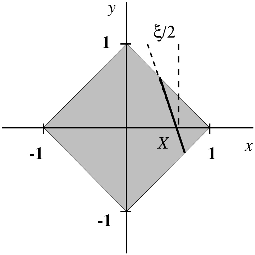
Figure 1: The range of the variables $x$ and $y$ in the double distribution, Eq.(19). The reduction to the skewed distribution, $H(X,\xi)$, is achieved by integrating the double distribution over the line $x+y\xi/2=X$, cf. Eq.(21), shown here for the case that $X>\xi/2$ (thick line).

see Fig.1. The property Eq.(11) implies that [25]

$$F^{I=0,1}(x,y;t) = F^{I=0,1}(x,-y;t).$$ (20)

The skewed distribution, Eq.(13), is obtained as a one–dimensional “section” of this two–variable function, imposing a particular “skewedness”, $\xi$:

$$\int_{-1}^{1}dx\int_{-(1-|x|)}^{1-|x|}dy\;\delta(X-x-y\xi/2)\,F^{I=0,1}(x,y;t) = H^{I=0,1}(X,\xi;t).$$ (21)

This reduction process is illustrated in Fig.1. In particular, in the forward limit the usual quark/antiquark distribution is recovered as

$$\int_{-(1-|X|)}^{1-|X|}dy\;F^{I=0}(X,y;t=0) = \frac{1}{2}\left[\theta(X)\,q_{\rm s}(X)\;-\;\theta(-X)\,q_{\rm s}(-X)\right]$$ (22)

and similarly for the isovector component, cf. Eq.(15).

The main reason for interest in a double distribution representation is the possibility to relate skewed distributions with different values of $\xi$. With certain assumptions about the behavior of the double distribution a number of statements about the skewed distributions follow immediately from the reduction formula, Eq.(21); see Refs.[4, 5] for an extensive discussion. For instance, if the double distribution were continuous everywhere on its region of support (see Fig.1), the skewed distribution would be a continuous function of $x$ and $\xi$. The double distribution is also convenient for model building, since any model of the double distribution, when inserted in the reduction formula, produces skewed distributions satisfying the polynomiality condition for the moments [4, 5, 25, 26]. However, in order to be practically relevant, such applications require understanding of the general behavior of the double distributions, in particular, of their possible singularities.

2.2 Trouble with double distributions

When discussing properties of double distributions (such as their singularities) one should keep in mind that the behavior of these functions is determined by the behavior of the matrix element, Eq.(6), as a function of $p\!\cdot\!z$ and $r\!\cdot\!z$, as well as by the particular way in which one writes the spectral representation for it. This concerns, in particular, the number of independent “twist–2 structures” one takes into account in the decomposition of the matrix element. We shall argue now that it is not always adequate to represent the pion non-forward matrix element in the form of Eq.(19), as a double spectral integral with a single prefactor, $p\!\cdot\!z$. This form is incompatible with general features of the dependence of the isoscalar matrix element, Eq.(6), on $p\!\cdot\!z$ and $r\!\cdot\!z$, and insisting on it one would incur severe singularities in the double distribution.

In order to obtain information about the behavior of the function ${\cal M}(p\!\cdot\!z,r\!\cdot\!z,t)$, Eq.(6), it is useful to consider instead of Eq.(6) the more general matrix element of the non-local vector operator [isospin components are defined in analogy to Eq.(6)]

$$\langle\pi(p-r/2)|\;\bar{\psi}(-z/2)\gamma_{\mu}\,[-z/2,z/2]\,\psi(z/2)\;|\pi(p+r/2)\rangle \equiv {\cal M}_{\mu}(p,r,z),$$ (23)

from which the matrix element Eq.(6) is obtained by contraction with the light–cone vector, $z^{\mu}$. On general grounds, this matrix element can be parametrized as (for both $I=0$ and $1$)

$${\cal M}_{\mu}(p,r,z) = 2p_{\mu}G\;+\;r_{\mu}G_{\parallel}\;+\;\mbox{term $\propto z_{\mu}$},$$ (24)

where $G$ and $G_{\parallel}$ are generalized form factors depending on $p\!\cdot\!z,r\!\cdot\!z$ and $t$. The terms proportional to $z_{\mu}$ vanish upon contraction with $z^{\mu}$ and does not contribute to the twist–2 part matrix element Eq.(6). The term proportional to $r_{\mu}$, however, does contribute to Eq.(6). In fact, it is the presence of this structure which causes trouble in the double–distribution representation of the isoscalar matrix element, Eq.(19).

In the limit $z\rightarrow 0$ the operator in Eq.(24) reduces to the local vector current, which is conserved. This implies that $G_{\parallel}(z=0)\equiv 0$ for all $t$, i.e., the matrix element is “transverse” ($\propto p_{\mu}$). However, the non-local operator with $z\neq 0$ is generally not conserved, so there is no reason for $G_{\parallel}$ to be zero for $z\neq 0$. Actually, current conservation is only a sufficient condition for $G_{\parallel}$ to be zero, not a necessary one. For $z=0$ one obtains $G_{\parallel}\equiv 0$ already from time reversal invariance and the hermiticity of the local current operator. Applying the same symmetry transformations to the non-local operator, one finds that for the isoscalar matrix element

$$G^{I=0}(p\!\cdot\!z,\,\,r\!\cdot\!z,\,\,t) = \;\;\;G^{I=0}(p\!\cdot\!z,\,\,-r\!\cdot\!z,\,\,t),$$

$$G_{\parallel}^{I=0}(p\!\cdot\!z,\,\,r\!\cdot\!z,\,\,t) = -G_{\parallel}^{I=0}(p\!\cdot\!z,\,\,-r\!\cdot\!z,\,\,t).$$ (25)

In the local case $r\!\cdot\!z=0$, and $G^{I=0}_{\parallel}$ would be zero identically in $t$. However, in the general case, $z\neq 0$, there is again no reason for $G_{\parallel}^{I=0}$ to be zero.

The presence of a “longitudinal” ($\propto r_{\mu}$) part of the vector matrix element, Eq.(24), means that the matrix element ${\cal M}^{I=0}$, obtained by contracting Eq.(24) with $z^{\mu}$, contains in addition to the $p\!\cdot\!z$–term a piece with prefactor $r\!\cdot\!z$,

$${\cal M}^{I=0}(p\!\cdot\!z,r\!\cdot\!z,t) = p\!\cdot\!z\,G^{I=0}(p\!\cdot\!z,r\!\cdot\!z,t)\;+\;r\!\cdot\!z\,G_{\parallel}^{I=0}(p\!\cdot\!z,r\!\cdot\!z,t).$$ (26)

In particular, since generally $G_{\parallel}^{I=0}\neq 0$, ${\cal M}$ does not vanish in the limit $p\!\cdot\!z\rightarrow 0$ and $r\!\cdot\!z\neq 0$:

$${\cal M}^{I=0}(p\!\cdot\!z\rightarrow 0,r\!\cdot\!z\neq 0,t) \neq 0.$$ (27)

One can easily see that this implies that the matrix element ${\cal M}^{I=0}$ cannot be represented in the form Eq.(19) with a non-singular double distribution $F^{I=0}(x,y)$. Suppose $F^{I=0}(x,y)$ were non-singular in its range of support. It would then define the matrix element on the L.H.S. as an analytic function of the variables $p\!\cdot\!z$ and $r\!\cdot\!z$, which could be continued to a point (in the unphysical region) where $p\!\cdot\!z=0$, but $r\!\cdot\!z\neq 0$. At this point the R.H.S. of Eq.(19) vanishes because of the prefactor $p\!\cdot\!z$, but not the matrix element on the L.H.S., cf. Eq.(27). Clearly, this implies that $F^{I=0}(x,y)$ must be singular, in one way or another.

What would be the character of these singularities? Trying to absorb a $p\!\cdot\!z$–independent piece in the integral Eq.(19) would amount to finding an integral representation of $1/p\!\cdot\!z$ in the form

$$\frac{1}{p\!\cdot\!z} = \int_{-1}^{1}dx\;e^{-ixp\!\cdot\!z}\;f(x),$$ (28)

with $f(x)$ some generalized function. Assuming that the integral on the R.H.S. can be continued to $p\!\cdot\!z\rightarrow 0$, one concludes that no Mellin moments of the function $f(x)$ exist. In particular, this means that the singularity in $f(x)$ cannot be of delta–function type. (We shall return to this point below.) Thus, we conclude that, although the two contributions to ${\cal M}^{I=0}$ in Eq.(26) are not structurally distinct, it is not possible to include the $r\!\cdot\!z$–term in a double distribution representation of the form Eq.(19) staying within the usual class of generalized functions.

It is important to mention that the difficulties noted here do not concern the representation of the matrix element through a skewed distribution, Eq.(13). In this case one writes the representation of the matrix element under the condition $r\!\cdot\!z=\xi p\!\cdot\!z$, with $\xi$ fixed. In particular, repeating the above argument and taking in Eq.(13) the limit $p\!\cdot\!z\rightarrow 0$ we would now also have $r\!\cdot\!z\rightarrow 0$, so that both L.H.S. and R.H.S. of Eq.(13) would vanish, and there is no need for $H^{I=0}$ to be singular.

Since there are many advantages in a double–distribution representation of the non-forward matrix elements, it is worthwhile to think how Eq.(19) could be modified to allow for a double spectral representation in terms of standard generalized function. The origin of the problems with the form Eq.(19) is that the matrix element does not go to zero in the limit $p\!\cdot\!z\rightarrow 0$, Eq.(27). One possibility would be to simply omit the prefactor $p\!\cdot\!z$ in Eq.(19); however, this would result in a function $F^{I=0}(x,y)$ which does not reduce to the usual parton distribution in the forward limit, $r\rightarrow 0$, cf. Eq.(22), and would not be useful for model building. Alternatively, one could add to Eq.(19) a term not vanishing in the limit $p\!\cdot\!z\rightarrow 0$. Minimally, this could be a term depending only on $r\!\cdot\!z$, which can be represented by a one–dimensional spectral integral:

$${\cal M}^{I=0}(p\!\cdot\!z,\,\,r\!\cdot\!z;t) = 2p\!\cdot\!z\,\int_{-1}^{1}dx\;e^{-ixp\!\cdot\!z}\;\int_{-(1-|x|)}^{1-|x|}dy\;e^{-iyr\!\cdot\!z/2}\;F^{I=0}(x,y;t)$$ (29)

$$+\;\;r\!\cdot\!z\,\int_{-1}^{1}dy\;e^{-iyr\!\cdot\!z/2}\;D(y;t).$$

The functions $F^{I=0}(x,y;t)$ and $D(y;t)$ are uniquely defined if we understand the first term to be a representation of ${\cal M}^{I=0}(p\!\cdot\!z,r\!\cdot\!z;t)-{\cal M}^{I=0}(0,r\!\cdot\!z;t)$, the second of ${\cal M}^{I=0}(0,r\!\cdot\!z;t)$, i.e., as a “subtraction term”. The explicit factor $r\!\cdot\!z$ in front of the second term is natural since ${\cal M}^{I=0}(0,r\!\cdot\!z\rightarrow 0)=0$. The support of $D$ is limited to $-1\leq y\leq 1$, i.e., this function has the character of a distribution amplitude. Time reversal and hermiticity, Eq.(25), require that (same $t$)

$$F^{I=0}(x,y) = F^{I=0}(x,-y),\hskip 56.9055ptD(y)\;\;=\;\;-D(-y),$$ (30)

i.e., the behavior with respect to $y\rightarrow-y$ of the new function $D(y)$ is opposite to that of the usual double distribution, Eq.(20).

The skewed distribution which follows from the new representation Eq.(29) is now the sum of two contributions:

$$H^{I=0}(X,\xi;t) = \int_{-1}^{1}dx\int_{-(1-|x|)}^{1-|x|}dy\;\delta(X-x-y\xi/2)\;F^{I=0}(x,y;t)$$ (31)

$$\;+\;\;\mbox{sign}(\xi)\,D\left(\frac{2X}{\xi};t\right).$$

Note that both contributions are even functions of $\xi$, in accordance with the general symmetry of the skewed distribution following from Eq.(11). The first piece follows the usual reduction formula, Eq.(21), and is generally non-zero in the entire range $-1<X<1$. The second piece is obtained by substituting in Eq.(29) $r\!\cdot\!z=\xi p\!\cdot\!z$ and changing the integration variable to $\xi y/2$. Since the support of $D$ is limited to $-1\leq y\leq 1$ this contribution to the skewed distribution is present only for $-\xi/2\leq X\leq\xi/2$. Thus, the need to include the “subtraction term” in the double distribution representation naturally leads to a skewed distribution with essentially different behavior in the regions $|X|<\xi/2$ and in $|X|>\xi/2$.

So far we have explored the consequences of the presence of “longitudinal” terms in the matrix element Eq.(24), or of property Eq.(27), from a general point of view, arguing that there is no reason for such contribution to be zero. In Section 3 we perform a model calculation of the pion matrix elements at a low normalization point in the effective chiral theory based on the instanton vacuum, wich shows that such terms in the matrix element do indeed appear, and lead to the “two–component” form of the skewed distribution described above.

The region $p\!\cdot\!z\rightarrow 0$ and $r\!\cdot\!z\neq 0$ implied in the limit in Eq.(27) corresponds to values of $|\xi|>2$, which are not physically accessible in DVCS. However, using crossing invariance one can relate the function ${\cal M}(p\!\cdot\!z,r\!\cdot\!z)$ in the unphysical region, Eq.(27), to the matrix element for two–pion production by a light–ray operator in the physical region (see Section 4). The latter can be measured (e.g. in $\gamma^{\ast}\gamma\rightarrow\pi\pi$ and $\gamma^{\ast}N\rightarrow\pi\pi N$ reactions) and is generally non-zero, providing additional evidence for the presence of $r\!\cdot\!z$–terms and the property Eq.(27).

A simple dynamical explanation for the origin of $r\!\cdot\!z$–terms in the isoscalar pion matrix element can be found by considering “resonance exchange” contributions to the matrix element, in the spirit of the vector dominance model for the pion electromagnetic form factor [38]. By this we mean “factorized” contributions to the matrix element in which the pion and the light–ray operator communicate by $t$–channel exchange of a resonance characterized by a twist–2 distribution amplitude, as are shown schematically in Fig.2. In Appendix B we derive a general formula describing the contribution resulting from the exchange of a resonance of arbitrary spin to the pion matrix element. In particular, we show there that the property Eq.(27) of the isoscalar matrix element is naturally obtained from exchange of even–spin isoscalar resonances. Far from being a complete dynamical description of the non-forward matrix element, this phenomenological model helps to develop an intuitive understanding why the structures described above appear.

The double distribution $F^{I=0}(x,y)$ in Eq.(29) is a generalized function which may contain delta function type singularities. Such terms in the double distribution [in the restricted ansatz Eq.(19)] were studied by Radyushkin in connection with resonance exchange contributions to the non-forward nucleon matrix elements [5, 26]. We already argued above that the pure $r\!\cdot\!z$–terms in the isoscalar pion matrix element, cf. Eq.(27), cannot be described by delta function type contributions to $F^{I=0}(x,y)$. It is interesting to verify this at the level of the reduction formula, Eq.(31). Could delta function contributions to $F^{I=0}(x,y)$ mock up the structure of the $D$–term in $H^{I=0}$? A term in $F^{I=0}(x,y)$ of the form $\delta(x)\phi(y)$ would give a contribution to the skewed distribution $H^{I=0}\propto\phi(2X/\xi)\,/|\xi|$, which is ruled out because $H^{I=0}$ must at the same time be odd in $X$ and even in $\xi$. One thus has to turn to derivatives of $\delta(x)$. A term $\delta^{\prime}(x)\chi(y)$ would give a contribution $H^{I=0}\propto\mbox{sign}(\xi)\,\chi^{\prime}(2X/\xi)\,/\xi^{2}$, which can be non-zero but cannot describe the contribution generated by $D(y)$ in Eq.(31) (consider for example the forward limit). This argument can easily be extended to any derivative of $\delta(x)$. Thus, we conclude that the term generated by $D(y)$ in Eq.(29) represents a genuine separate structure which cannot be obtained from delta function contributions to $F^{I=0}(x,y)$.

We remark that in the resonance exchange model of Appendix B exchange of even–spin resonances generally contributes to both $D(y)$ and to delta function terms in $F^{I=0}(x,y)$, cf. Eq.(B.6). Spin–0 (“sigma meson”) exchange is special in that it contributes only to $D(y)$.

In the amplitude for hard exclusive processes such as DVCS the skewed distribution is convoluted with a hard scattering kernel which is singular at $X=\pm\xi/2$ [2, 3, 4, 5]. For this integral to exist (i.e., for factorization to hold) it is important that the skewed distribution be continuous in $X$ at these points. Assuming that the first term on the R.H.S. of Eq.(31) is continuous, this would be satisfied if

$$D(y;t) \rightarrow 0\hskip 42.67912pt(y\rightarrow\pm 1).$$ (32)

We shall see below that it is indeed reasonable to expect that $D(y;t)$ satisfies this property, reminiscent of a meson distribution amplitude. Model calculations of the matrix elements in the effective chiral theory bases on the instanton vacuum and in a “resonance exchange” model give rise to functions satisfying Eq.(32).

The representation Eq.(29) is the minimal modification of Eq.(19) consistent with Eq.(27). For some purposes (e.g. crossing symmetry) it could be convenient to have a representation which is symmetric with respect to $p\!\cdot\!z$ and $r\!\cdot\!z$. One could write:

$${\cal M}^{I=0}(p\!\cdot\!z,\,\,r\!\cdot\!z) = 2p\!\cdot\!z\,\int_{-1}^{1}dx\;e^{-ixp\!\cdot\!z}\;\int_{-(1-|x|)}^{1-|x|}dy\;e^{-iyr\!\cdot\!z/2}\;F^{I=0}(x,y)$$ (33)

$$+\;\;r\!\cdot\!z\,\int_{-1}^{1}dx\;e^{-ixp\!\cdot\!z}\;\int_{-(1-|x|)}^{1-|x|}dy\;e^{-iyr\!\cdot\!z/2}\;F_{\parallel}^{I=0}(x,y).$$

The two functions $F^{I=0}$ and $F^{I=0}_{\parallel}$ would be uniquely determined if we defined them as the spectral representation of the generalized form factors $G^{I=0}(p\!\cdot\!z,r\!\cdot\!z,t)$ and $G^{I=0}_{\parallel}(p\!\cdot\!z,r\!\cdot\!z,t)$ of the vector operator, Eq.(24). Again, Eq.(25) requires that

$$F^{I=0}(x,y) = F^{I=0}(x,-y),\hskip 56.9055ptF_{\parallel}^{I=0}(x,y)\;\;=\;\;-F_{\parallel}^{I=0}(x,-y).$$ (34)

In terms of these new functions the skewed distribution would now be given by the reduction formula Eq.(21) with

$$F(x,y) \rightarrow F(x,y)\;+\;\frac{\xi}{2}\,F_{\parallel}(x,y).$$ (35)

Note that both $F$ and $F_{\parallel}$ are generalized functions which may contain delta–function singularities.

Finally, let us note that for the isovector pion matrix element, ${\cal M}^{I=1}$, the original form of the double distribution representation, Eq.(19), works fine, and no “subtraction terms” of the kind in Eq.(29) are required. This is because ${\cal M}^{I=1}$ is odd in $p\!\cdot\!z$ for any $r\!\cdot\!z$ and t [as follows from combining Eq.(10) and Eq.(11)], and thus

$${\cal M}^{I=1}(p\!\cdot\!z\rightarrow 0,r\!\cdot\!z\neq 0,t) \rightarrow 0.$$ (36)

In the resonance exchange model this is again easily understood; it follows from the fact that isovector two–pion resonances have odd spin, see Eq.(B.6) in Appendix B.

2.3 The nucleon

We now turn to non-forward matrix elements in the nucleon. By a simple extension of the arguments offered in the previous subsection for the pion, we show that also in the case of the nucleon the double distribution representation of Refs.[4, 5, 26] should be modified to take into account all possible twist–2 structures.

The object of interest now is the nucleon matrix element of the twist–2 light ray operator of Eq.(6). Again we distinguish the isoscalar and isovector matrix elements:

$$\langle N(p-r/2),T_{3}^{\prime},\lambda^{\prime}|\;\bar{\psi}(-z/2)\left\{\begin{array}[]{c}1\\[8.61108pt] \tau^{c}\end{array}\right\}\hat{z}\,[-z/2,z/2]\,\psi(z/2)\;|N(p+r/2),T_{3},\lambda\rangle$$ (39)

$$= \left\{\begin{array}[]{r}2\delta_{T_{3}T_{3}^{\prime}}\;{\cal M}^{I=0}({\lambda^{\prime},\lambda};p\!\cdot\!z,\,\,r\!\cdot\!z;\,\,t)\\[8.61108pt] 2\left(\tau^{c}\right)_{T_{3}T_{3}^{\prime}}{\cal M}^{I=1}({\lambda^{\prime},\lambda};p\!\cdot\!z,\,\,r\!\cdot\!z;\,\,t),\end{array}\;\;\;\;\;\right.$$ (42)

where $T_{3},T_{3}^{\prime}$ denote the isospin projection ($T_{3},T_{3}^{\prime}=\pm 1/2$ for proton/neutron). The only difference to the pion is that now the functions ${\cal M}^{I=0,1}$ depend also on the helicities of the incoming ($\lambda$) and outgoing ($\lambda^{\prime}$) nucleon. In analogy to the pion, Eq.(24), let us consider also the matrix element of the more basic light–ray operator with $\gamma_{\mu}$ [the isospin decomposition is analogous to Eq.(42) and not written],

$$\langle N(p-r/2),\lambda^{\prime}|\;\bar{\psi}(-z/2)\gamma_{\mu}\,[-z/2,z/2]\,\psi(z/2)\;|N(p+r/2),\lambda\rangle \equiv {\cal M}_{\mu}(\lambda^{\prime},\lambda;p,r,z),$$

which on general grounds can be parametrized as (for both $I=0$ and $1$)

$${\cal M}_{\mu} = \bar{U}^{\prime}\left[\gamma_{\mu}\;G_{1}\;+\;\frac{i}{2M_{N}}\sigma_{\mu\nu}r^{\nu}G_{2}\;+\;r_{\mu}G_{\parallel}\;+\;\ldots\right]U$$ (44)

where $\bar{U}^{\prime}\equiv\bar{U}(p-r/2,\lambda^{\prime}),\;\;U\equiv U(p+r/2,\lambda)$ are the nucleon spinors. We have not written explicitly terms which vanish upon contraction with $z^{\mu}$ and do not contribute to the twist–2 part (such as $z_{\mu},\,\sigma_{\mu\nu}z^{\nu}$). Here $G_{1},G_{2},G_{\parallel}$ are generalized form factors depending on $p\!\cdot\!z,r\!\cdot\!z$ and $t$. In the limit of a local operator, $z\rightarrow 0$, $G_{1}$ and $G_{2}$ reduce to the usual Dirac form factors for the vector current, and $G_{\parallel}\rightarrow 0$ because of current conservation. However, as in the case of the pion, for $z\neq 0$ the term $\propto r_{\mu}$ is generally non-zero, $G_{\parallel}\neq 0$.

Contracting Eq.(44) with $z^{\mu}$ we obtain the twist–2 matrix element, Eq.(42) (for both $I=0$ and $1$):

$${\cal M}(\lambda^{\prime},\lambda;p\!\cdot\!z,\,\,r\!\cdot\!z;t) = \bar{U}^{\prime}\left[\hat{z}\;G_{1}\;+\;\frac{i}{2M_{N}}\sigma_{\mu\nu}z^{\mu}r^{\nu}G_{2}\;+\;r\!\cdot\!zG_{\parallel}\right]U.$$ (45)

Actually, here the three structures are not independent. Using the well–known identity

$$\bar{U}^{\prime}Up_{\mu} = 2M_{N}\bar{U}^{\prime}\gamma_{\mu}U\;+\;i\bar{U}^{\prime}\sigma_{\mu\nu}Ur^{\nu},$$ (46)

we could rewrite the third term as a linear combination of the first two. In this way we would arrive at ($I=0,1$):

$${\cal M}(\lambda^{\prime},\lambda;p\!\cdot\!z,\,\,r\!\cdot\!z;t) = \bar{U}^{\prime}\left[\hat{z}\;\widetilde{G}_{1}\;+\;\frac{i}{2M_{N}}\sigma_{\mu\nu}z^{\mu}r^{\nu}\widetilde{G}_{2}\right]U,$$ (47)

where

$$\widetilde{G}_{1} = G_{1}\;+\;2\frac{r\!\cdot\!z}{p\!\cdot\!z}\,G_{\parallel},\hskip 56.9055pt\widetilde{G}_{2}\;\;=\;\;G_{2}\;+\;2\frac{r\!\cdot\!z}{p\!\cdot\!z}\,G_{\parallel}.$$ (48)

A decomposition of the form Eq.(47) was assumed in Refs.[4, 5], where a double distribution representation of the matrix element was proposed in the form

$${\cal M}^{I=0,1}(\lambda^{\prime},\lambda;p\!\cdot\!z,\,\,r\!\cdot\!z;t)$$ (49)

$$= \bar{U}^{\prime}\hat{z}U\,\int_{-1}^{1}dx\;e^{-ixp\!\cdot\!z}\;\int_{-(1-|x|)}^{1-|x|}dy\;e^{-iyr\!\cdot\!z/2}\;F^{I=0,1}(x,y;t)$$

$$+\;\;\frac{i}{2M_{N}}z^{\mu}r^{\nu}\bar{U}^{\prime}\sigma_{\mu\nu}U\,\int_{-1}^{1}dx\;e^{-ixp\!\cdot\!z}\;\int_{-(1-|x|)}^{1-|x|}dy\;e^{-iyr\!\cdot\!z/2}\;K^{I=0,1}(x,y;t).$$

We see that in the isoscalar case this ansatz suffers from the same problem as the simple ansatz for the double distribution in the pion, Eq.(19). Since in general $G^{I=0}_{\parallel}\neq 0$, the functions $\widetilde{G}^{I=0}_{1},\widetilde{G}^{I=0}_{2}$ in the reduced decomposition, Eq.(48), have singularities of the type $1/p\!\cdot\!z$, which cannot be represented by spectral integrals with usual generalized functions, as described in the previous subsection. Thus, the conclusion is the same as for the pion: Although the twist–2 contributions from the “longitudinal” part ($\propto r_{\mu}$) of the vector matrix element are not structurally distinct from those from the “transverse” part ($\propto p_{\mu}$), one cannot obtain them from a double distribution representation whose form is modeled on the “transverse” part.

Again we stress that there is no problem with a representation of the matrix element Eq.(47) in terms of skewed distributions (see Refs.[2, 3, 4, 5] for their definition in the nucleon). In this case the factors $r\!\cdot\!z/p\!\cdot\!z$ incurred in eliminating the $r\!\cdot\!z$–term, Eq.(48), are replaced by the skewedness, $\xi$, which is a fixed external parameter.

In analogy to the pion, Eq.(29), we suggest to modify the spectral representation Eq.(49) by explicitly including the $r\!\cdot\!z$–terms. A minimal variant would be to add a term depending only on $r\!\cdot\!z$, in which one could absorb the $p\!\cdot\!z$–independent part of the “longitudinal” term of Eq.(26), $r\!\cdot\!zG^{I=0}_{\parallel}(p\!\cdot\!z=0,r\!\cdot\!z)$:

$${\cal M}^{I=0}(\lambda^{\prime},\lambda;p\!\cdot\!z,\,\,r\!\cdot\!z;t)$$ (50)

$$= \bar{U}^{\prime}\hat{z}U\,\int_{-1}^{1}dx\;e^{-ixp\!\cdot\!z}\;\int_{-(1-|x|)}^{1-|x|}dy\;e^{-iyr\!\cdot\!z/2}\;F^{I=0}(x,y;t)$$

$$+\;\;\frac{i}{2M_{N}}z^{\mu}r^{\nu}\bar{U}^{\prime}\sigma_{\mu\nu}U\,\int_{-1}^{1}dx\;e^{-ixp\!\cdot\!z}\;\int_{-(1-|x|)}^{1-|x|}dy\;e^{-iyr\!\cdot\!z/2}\;K^{I=0}(x,y;t)$$

$$+\;\;\bar{U}^{\prime}U\,r\!\cdot\!z\,\int_{-1}^{1}dy\;e^{-iyr\!\cdot\!z/2}\;D(y;t).$$

Alternatively, one could directly work with the spectral representation of the form factors $G_{1},G_{2}$ and $G_{\parallel}$, as in the representation Eq.(33) for the pion.

The skewed distribution in the nucleon resulting from the full double distribution representation, Eq.(50), again has a “two–component” form, since the term with $D(y)$ gives rise to a contribution non-zero only in the region $-\xi/2\leq X\leq\xi/2$. (The corresponding reduction formulas can be obtained by a trivial modification of the ones written in Refs.[4, 5, 26].) This explains the behavior of the isoscalar skewed distribution, $H^{I=0}$, which was encountered in a model calculation in the large–$N_{c}$ limit [12].

3 Distributions in the pion from effective chiral dynamics

For quantitative estimates of the non-forward matrix elements Eq.(6) and the skewed and double distributions one has to turn to model calculations. Here we compute these quantities at a low normalization point in the low-energy effective field theory based on the instanton model of the QCD vacuum. This effective theory incorporates the dynamical breaking of chiral symmetry, and provides a realistic description of hadronic properties of the pion and nucleon [13, 28]. Its content can be summarized in an effective action describing the interaction of a pion field with massive “constituent” quarks, in a way which is dictated by chiral invariance:

$$S_{\rm eff} = \int d^{4}x\;\bar{\psi}(x)\left[i\hat{\partial}-MF(\partial^{2})\;e^{i\gamma_{5}\tau^{a}\pi^{a}(x)/F_{\pi}}\;F(\partial^{2})\right]\psi(x).$$ (51)

Here, $\pi^{a}$ is the pion field, and $F_{\pi}=93\,{\rm MeV}$ is the weak pion decay constant. The dynamical quark mass generated in the spontaneous breaking of chiral symmetry is momentum dependent; the form factors $F(\partial^{2})$ are related to the instanton zero modes [13]. They cut loop integrals at momenta of order of the inverse average instanton size, $\bar{\rho}^{-1}\approx 600\,{\rm MeV}$.

The effective theory Eq.(51) has been derived from the instanton model of the QCD vacuum. This allows for an unambiguous identification of the twist–2 QCD operators with operators in the effective theory. It is understood that the QCD operators are normalized at a scale of the order $\mu=\bar{\rho}^{-1}\approx 600\,{\rm MeV}$. The general framework for computing parton distributions and meson wave functions at a low normalization point within this approach has been developed in Refs.[14, 15]. An essential point is that the value of the dynamical quark mass, $M$, is parametrically small compared to the UV cutoff, $\bar{\rho}^{-1}$; their ratio is proportional to the packing fraction of the instanton medium $(M\bar{\rho})^{2}\sim(\bar{\rho}/\bar{R})^{4}$. Qualitatively speaking this means that in leading order in this parameter one is dealing with structureless constituent quarks; in particular, the gluon distribution appears only at order $(M\bar{\rho})^{2}$. At a technical level, working in leading order in $M\bar{\rho}$ means retaining only the ultraviolet divergent part of the quark loop integrals computed with Eq.(51), absorbing the ultraviolet divergence in the pion decay constant, $F_{\pi}$.

The non-linear form of the coupling of the pion to the quarks in Eq.(51) is required by chiral invariance. Expanding the exponential in powers of the pion field we obtain

$$e^{i\gamma_{5}\tau^{a}\pi^{a}(x)/F_{\pi}} = 1\;+\;\frac{i}{F_{\pi}}\gamma_{5}\pi^{a}(x)\tau^{a}\;-\;\frac{1}{2F_{\pi}^{2}}\pi^{a}(x)\pi^{a}(x)\;\;+\;\;\ldots,$$ (52)

The effective theory contains a Yukawa–type quark–pion vertex as well as a two–pion quark vertex. Consequently, there are in general two contributions to the matrix element of a twist–2 quark operator between pion states, corresponding to the diagrams (a) and (b) of Fig.3. The diagram (a) of Fig.3 contributes only to the flavor–singlet matrix element, while (b) contributes both in the flavor–singlet and non–singlet case. The Feynman integrals can straightforwardly be computed introducing light–cone coordinates with respect to the vector $n\sim z$; see Refs.[15, 16, 18] for details. The integral over transverse momenta contains a logarithmic divergence which is cut by the form factors, $F(\partial^{2})$. More simply, one may keep only the logarithmically divergent part of the diagram and absorb the logarithmic divergence in the pion decay constant. It was shown in Refs.[12, 16] that this is a legitimate approximation except in the vicinity $X=\pm\xi/2$. (We shall include the form factors in the calculation later.)

In this approximation the contributions of diagrams (a) and (b) of Fig.3 to the matrix elements, Eq.(6), can be computed analytically. For the isoscalar part we obtain (for simplicity we take $t\rightarrow 0$):

$${\cal M}^{I=0}(p\!\cdot\!z,r\!\cdot\!z)^{\rm(a)} = 2i\,\left[-\cos\frac{r\!\cdot\!z}{2}+\frac{2}{r\!\cdot\!z}\sin\frac{r\!\cdot\!z}{2}\right],$$ (53)

$${\cal M}^{I=0}(p\!\cdot\!z,r\!\cdot\!z)^{\rm(b)} = 2i\,\left[\cos p\!\cdot\!z-\frac{2}{r\!\cdot\!z}\sin\frac{r\!\cdot\!z}{2}\right]$$ (54)

and the total result is

$${\cal M}^{I=0}(p\!\cdot\!z,r\!\cdot\!z) = 2i\,\left[\cos p\!\cdot\!z-\cos\frac{r\!\cdot\!z}{2}\right].$$ (55)

Here contribution $(a)$ depends only on $r\!\cdot\!z$; due to the contact nature of the two–pion–quark vertex, Eq.(52), the average momentum $p$ does not enter in the quark loop, see Fig.3. This contribution vanishes in the forward limit $r\rightarrow 0$. Note that both contributions to the isoscalar matrix element, as well as their total, behave as described in Section 2: they do not go to zero in the limit $p\!\cdot\!z\rightarrow 0,\;r\!\cdot\!z\neq 0$, and thus cannot be represented by a double distribution in the form Eq.(19). Within the proposed new representation, Eq.(29), which allows for a $p\!\cdot\!z$–independent part, this model result would correspond to

$$F^{I=0}(x,y) = \frac{1}{2}\left[\theta(-1<x<0)\;-\;\theta(0<x<1)\right]\,\,\delta(y),$$ (56)

$$D(y) = \frac{1}{2}\left[-\theta(-1<y<0)\;+\;\theta(0<y<1)\right],$$ (57)

where $\theta(a<X<b)$ is unity if $a<X<b$ and else zero. That $F^{I=0}$ here is proportional to a delta function in $y$ should be seen as an artifact of keeping only the logarithmically divergent piece; this would change when retaining finite terms at $t\neq 0$.

The result for the isovector matrix element, Eq.(6), at $t\rightarrow 0$ is

$${\cal M}^{I=1}(p\!\cdot\!z,r\!\cdot\!z) = {\cal M}^{I=1}(p\!\cdot\!z,r\!\cdot\!z)^{\rm(b)}\;\;=\;\;4\sin p\!\cdot\!z.$$ (58)

This matrix element vanishes in the limit $p\!\cdot\!z\rightarrow 0$, hence there is no problem with representing it by a double distribution in the form Eq.(19):

$$F^{I=1}(x,y) = \theta(-1<x<1)\,\delta(y).$$ (59)

The corresponding skewed distributions may be computed either using the results for the matrix elements, Eqs.(53) and (54), and the definition Eq.(13), or directly by computing the R.H.S. of Eq.(14); both ways lead to identical results. For the isoscalar part we find

$$H^{I=0}(X,\xi)^{\rm(a)} = -\frac{1}{2}\,\,\theta\left(-\frac{\xi}{2}<X<\frac{\xi}{2}\right)\frac{2X}{\xi},$$ (60)

$$H^{I=0}(X,\xi)^{\rm(b)} = \frac{1}{2}\left[-\theta\left(-1<X<-\frac{\xi}{2}\right)\;+\;\theta\left(-\frac{\xi}{2}<X<\frac{\xi}{2}\right)\frac{2X}{\xi}\right.$$ (61)

$$\left.\;\;\;\;+\;\theta\left(\frac{\xi}{2}<X<1\right)\right];$$

the total result is

$$H^{I=0}(X,\xi) = \frac{1}{2}\left[-\theta\left(-1<X<-\frac{\xi}{2}\right)\;+\;\theta\left(\frac{\xi}{2}<X<1\right)\right].$$ (62)

The functions are shown in Fig.4. One sees that the contribution from diagram (a), Eq.(60), is non-zero only in the region $-\xi/2<X<\xi/2$. It is absent in the forward limit, $r\rightarrow 0$. Note that this contribution to the skewed distribution is discontinuous in $X$ at $\pm\xi/2$; this behavior will be modified when taking into account the momentum dependence of the dynamical quark mass, see below. The contribution from diagram (b) is continuous at $X=\pm\xi/2$; this part reduces in the forward limit, $\xi\rightarrow 0$, to the singlet quark distribution in the pion, Eq.(15), which in this approximation (keeping only the logarithmic divergence, neglecting the form factors) would simply be given by

$$q_{\rm sing}(x) = \theta(0<X<1).$$ (63)

The result Eq.(62) is consistent with the generalized momentum sum rule, Eq.(17). In our approach based on the instanton vacuum the gluon distribution is parametrically small, $\propto(M\bar{\rho})^{2}\sim(\bar{\rho}/\bar{R})^{4}$, so the skewed quark distribution, Eq.(62), should saturate the sum rule at the low normalization point. Integrating Eq.(62) we observe that, indeed,

$$\int_{-1}^{1}dX\,X\,H^{I=0}(X,\xi) = \frac{1}{2}\left(1\;-\;\frac{\xi^{2}}{4}\right).$$ (64)

Eqs.(60), (61) and (62) represent the result for the skewed distribution obtained without taking into account the momentum dependence of the dynamical quark mass. The discontinuity at $X=\pm\xi/2$ in the contribution (a) to $H^{I=0}$ obtained in this approximation would violate the factorization of the DVCS amplitude, since the hard scattering kernel contains poles at $X=\pm\xi/2$. However, as was shown in Refs.[12], the momentum dependence of the dynamical quark mass can not be neglected for values of $X$ near $\pm\xi/2$, since in this case the integral over transverse momenta is cut by the form factors already at momenta of order $M\ll\bar{\rho}^{-1}$. The same mechanism makes the pion distribution amplitude vanish at the end points [15]. In Fig.4 we show the two contributions (a) and (b) to $H^{I=0}$ obtained when taking into account the form factors $F(\partial^{2})$ (we use the simple analytic approximation of Eq.(24) of Ref.[15]). As expected, contribution (a) now vanishes at $X=\pm\xi/2$, while the modification of contribution (b), which was continuous already without form factors, is only quantitative.

Finally, the result for the isovector skewed distribution at $t\rightarrow 0$ is

$$H^{I=1}(X,\xi) = H^{I=1}(X,\xi)^{\rm(b)}\;\;=\;\;\theta\left(-1<X<1\right),$$ (65)

which is an even function of $X$, in agreement with $C$–invariance. [In the forward limit this corresponds to a valence quark distribution in the pion $q_{\rm v}(X)=\theta\left(0<X<1\right)$, cf. Eq.(15), so comparing with Eq.(63) we see that in this approximation (no form factors) the “sea” quark distribution in the pion is zero.] As in the case of contribution (b) to the isoscalar distribution, inclusion of the form factors $F(\partial^{2})$ does not change the result for the isovector skewed distribution in an essential way, except for forcing the distribution to vanish at $X=\pm 1$.

Some comments are in order concerning the calculation of skewed and double distributions in the nucleon. In the large–$N_{c}$ limit the nucleon in the effective low–energy theory is characterized by a classical pion field (“soliton”) [28]. Quantization of the translational and rotational zero modes in the framework of the $1/N_{c}$–expansion gives rise to nucleon states with definite momentum and spin/isospin quantum numbers. When applying this approach to the computation of non-forward matrix elements of the type Eq.(6), the standard $1/N_{c}$–expansion implies that different components of the average momentum, $p$, and momentum transfer, $r$, are of different order in $N_{c}$ [the nucleon mass is $O(N_{c})$, while the momentum transfer in the Breit frame is $O(N_{c}^{0})$]. While it is possible to compute the skewed distribution, Eq.(14), in the parametric range $X,\xi\sim 1/N_{c}$ [12], it is not possible to uniformly obtain the matrix element Eq.(6) in the whole kinematical range necessary to restore the double distribution. In contrast, in the case of the pion all components of $p$ and $r$ are $O(N_{c}^{0})$, making it possible to treat $p$ and $r$ on the same footing.

4 Crossing and the two–pion distribution amplitude

4.1 Two–pion distribution amplitude

An interesting feature of the pion is the fact that the quantity related to the skewed parton distribution by crossing, namely the two–pion distribution amplitude (DA), can be measured in two–pion production at low invariant masses. These $2\pi$DA’s were introduced recently in the context of the QCD description of the process $\gamma^{\ast}\gamma\to 2\pi$ [17]. We now establish explicitly their relation to the skewed quark distributions in the pion. This will allow us to express the $t$–dependence of the lowest moments of the skewed distribution in terms of form factors in the timelike region.

The two–pion DA’s are defined, in analogy to the skewed parton distribution, as the matrix elements of the twist–2 operators between the vacuum and a two–pion state:

$${}_{\rm out}\langle\pi^{a}(p_{1})\pi^{b}(p_{2})|\;\bar{\psi}(-z/2)\left\{\begin{array}[]{c}1\\[8.61108pt] \tau^{c}\end{array}\right\}\hat{z}\,[-z/2,z/2]\,\psi(z/2)\;|0\rangle$$ (68)

$$= P\cdot z\;\int_{0}^{1}du\;e^{i(u-1/2)P\cdot z}\;\left\{\begin{array}[]{r}2\delta^{ab}\;\Phi^{I=0}(u,\zeta,W^{2})\\[8.61108pt] 2i\varepsilon^{abc}\;\Phi^{I=1}(u,\zeta,W^{2}).\end{array}\right.\;$$ (71)

The outgoing pions have momenta $p_{1},p_{2}$, and $P\equiv p_{1}+p_{2}$ is the total momentum of the final state. The generalized DA’s, Eq. (71), depend on the following kinematical variables: the quark momentum fraction with respect to the total momentum of the two–pion state, $z$; the variable $\zeta\equiv(z\cdot p_{1})/(z\cdot P)$ characterizing the distribution of longitudinal momentum between the two pions, and the invariant mass of the two–pion system, $W^{2}=P^{2}$. Also, an explicit representation of the DA can be written in analogy to Eq.(14) [the isospin decomposition is analogous to Eq.(71)]

$$\Phi(u,\zeta,W^{2})\;\;=\;\;\frac{1}{2}\int\frac{d\tau}{2\pi}e^{-i\tau(u-1/2)\,p\cdot n}$$ (72)

$$\times{}_{\rm out}\langle\pi(p_{1})\pi(p_{2})|\;\bar{\psi}(-\tau n/2)\,\,\hat{n}\,\,[-\tau n/2,\tau n/2]\,\psi(\tau n/2)\;|0\rangle,$$

where $n\propto z$ is a dimensionless light–like vector.

From $C$–parity one derives the following symmetry properties (we do not write the argument $W^{2}$):

$$\Phi^{I=0}(u,\zeta) = -\Phi^{I=0}(1-u,\zeta)\;\;=\;\;\;\;\Phi^{I=0}(u,1-\zeta),$$

$$\Phi^{I=1}(u,\zeta) = \;\;\Phi^{I=1}(1-u,\zeta)\;\;=\;\;-\Phi^{I=1}(u,1-\zeta).$$ (73)

The first moment of the isovector ($I=1$) two–pion DA is the pion e.m. form factor in the time-like region,

$$\int_{0}^{1}du\;\Phi^{I=1}(u,\zeta,W^{2}) = (2\zeta-1)\,F_{\pi}^{{\rm e.m.}}(W^{2})\;,$$ (74)

and thus scale–independent ($F_{\pi}^{{\rm e.m.}}(0)=1$). For the isoscalar ($I=0$) part, however, we have the normalization condition [19, 30]

$$\int_{0}^{1}du\,(2u-1)\,\Phi^{I=0}(u,\zeta,W^{2}) = -2M_{2}^{(\pi)}\;\zeta(1-\zeta)\;F_{\pi}^{{\rm EMT}}(W^{2}),$$ (75)

where $M_{2}^{(\pi)}$ is the momentum fraction carried by quarks in the pion at the given scale, and $F_{\pi}^{{\rm EMT}}(W^{2})$ is the form factor of the quark part of the energy momentum tensor, normalized to $F_{\pi}^{{\rm EMT}}(0)=1$. In Ref. [19] this form factor was estimated in the instanton model of the QCD vacuum at low two-pion invariant mass:

$$F_{\pi}^{{\rm EMT}}(W^{2}) = 1\;+\;\frac{N_{c}W^{2}}{48\pi^{2}F_{\pi}^{2}}\;+\;\ldots\;.$$

It is useful to expand the two–pion DA simultaneously in eigenfunctions of the ERBL evolution equation [21] [Gegenbauer polynomials $C_{n}^{3/2}(2u-1)$] and in partial waves of the produced two–pion system [Legendre polynomials, or Gegenbauer polynomials $C_{l}^{1/2}(2\zeta-1)$]. Generically this decomposition is of the form [19]:

$$\Phi(u,\zeta,W^{2}) = 6u(1-u)\;\sum_{n=0}^{\infty}\sum_{l=0}^{n+1}B_{nl}(W^{2})\;C_{n}^{3/2}(2u-1)\;C_{l}^{1/2}(2\zeta-1),$$ (76)

where $n$ runs over even (odd) and $l$ over odd (even) integers for the isovector (isoscalar) DA, cf. Eq. (73). The normalization condition Eq. (74) requires that $B_{01}^{I=1}(W^{2})\;=\;F_{\pi}^{{\rm e.m.}}(W^{2})$. Note that the asymptotic form of the isovector two–pion DA is given by [18]

$$\Phi^{I=1}_{\rm asymp}(u,\zeta,W^{2}) = 6u(1-u)\,(2\zeta-1)\;F_{\pi}^{{\rm e.m.}}(W^{2}).$$ (77)

In Ref. [19] certain soft–pion theorems for the two-pion DA were proven, which apply in the regions $\zeta\rightarrow 0$ or $\zeta\rightarrow 1$ and $W^{2}\rightarrow 0$, where one of the produced pions becomes soft. In the isovector case ($I=1$) they relate the two–pion DA to the DA of one pion, $\phi_{\pi}(u)$:

$$\Phi^{I=1}(u,\zeta=1,W^{2}=0) = -\Phi^{I=1}(u,\zeta=0,W^{2}=0)\;\;=\;\;\phi_{\pi}(u),$$ (78)

while in the the isoscalar case ($I=0$) one obtains

$$\Phi^{I=0}(u,\zeta=1,W^{2}=0) = \Phi^{I=0}(u,\zeta=0,W^{2}=0)\;\;=\;\;0.$$ (79)

The theorem Eq. (78) allows to relate the expansion coefficients of the isovector two–pion DA, Eq. (76), at $W^{2}=0$, with those of the pion DA,

$$\phi_{\pi}(u) = 6u(1-u)\;\left[1\;+\;\sum_{n\;{\rm even}}a_{n}^{(\pi)}\;C_{n}^{3/2}(2u-1)\right];$$ (80)

the relation takes the form

$$a_{n}^{(\pi)} = \sum_{l=1}^{n+1}\;B_{nl}^{I=1}(W^{2}=0).$$ (81)

4.2 Crossing relation

By crossing, the matrix element defining the two–pion DA, Eq.(72), is related to the one appearing in the definition of the skewed distribution, Eq.(14). This allows one to express the moments of the skewed parton distribution in terms of the expansion coefficients of the two–pion DA, Eq.(76). This relation takes the form:

$$\int_{-1}^{1}dX\,X^{N-1}\;H^{I}(X,\xi;t) = \sum_{n=0}^{N-1}\;\sum_{l=0}^{n+1}B^{I}_{nl}(t)\;\left(\frac{\xi}{2}\right)^{N}C_{l}^{1/2}\left(\frac{2}{\xi}\right)$$ (82)

$$\times\int_{0}^{1}du\;6u(1-u)\,(2u-1)^{N-1}\,C_{n}^{3/2}(2u-1).$$

One immediately notes that the R.H.S. is a polynomial of degree (at most) $N$ in $\xi$, i.e., the polynomiality condition for the skewed distribution (see Subsection 2.1 and Ref.[27]) is satisfied. Since only the $B_{nl}$ with $n$ odd (even) are non-zero in the isoscalar (isovector) case, the skewed distribution is an odd (even) function in $X$, in agreement with $G$–parity, Eq.(10). Also, note that due to the restrictions in the values of $l$, cf. Eq.(76), $H$ is an even function of $\xi$ for both $I=0$ and $1$, as it should be.

To prove the relation Eq.(82), we consider the expression for the $N-$th moment of the skewed distribution as a non-forward matrix element of a local spin–$N$, twist–2 operator,

$$\int_{-1}^{1}dX\,X^{N-1}\;H(X,\xi,t)$$ (83)

$$= (2p\!\cdot\!n)^{-N}\,\langle\pi(p+r/2)|\bar{\psi}\,n\!\cdot\!\gamma\;(n\cdot\stackrel{{\scriptstyle\leftrightarrow}}{{\nabla}})^{N-1}\,\psi|\pi(p-r/2)\rangle.$$

The $N$–th moments of the two–pion DA, Eq.(72), is given by the vacuum to two–pion matrix element of the same local operator. Substituting the double expansion, Eq.(76), we obtain

$$\int_{0}^{1}du\,(2u-1)^{N-1}\;\Phi(u,\zeta,W^{2})$$ (84)

$$= \left[(p_{1}+p_{2})\cdot n\right]^{-N}\;\langle\pi(p_{1})\pi(p_{2})|\bar{\psi}\,n\!\cdot\!\gamma\,(n\cdot\stackrel{{\scriptstyle\leftrightarrow}}{{\nabla}})^{N-1}\,\psi|0\rangle$$

$$= \sum_{n=0}^{N-1}\;\sum_{l=0}^{n+1}\;B^{I}_{nl}\left((p_{1}+p_{2})^{2}\right)\;C_{l}^{1/2}\left(\frac{n\!\cdot\!(p_{2}-p_{1})}{n\!\cdot\!(p_{2}+p_{1})}\right)$$

$$\times\int_{0}^{1}du\;6u(1-u)\,(2u-1)^{N-1}\,C_{n}^{3/2}(2u-1).$$

The matrix elements of the local operators are related to each other by usual crossing symmetry,

$$\langle p^{\prime}|\bar{\psi}\,n\!\cdot\!\gamma\;(n\cdot\stackrel{{\scriptstyle\leftrightarrow}}{{\nabla}})^{N-1}\,\psi|p\rangle = \langle p,-p^{\prime}|\bar{\psi}\,n\!\cdot\!\gamma\,(n\cdot\stackrel{{\scriptstyle\leftrightarrow}}{{\nabla}})^{N-1}\,\psi|0\rangle.$$ (85)

[In this shorthand expression, both sides are regarded as functions of the pion four–momenta, defined in the respective physical regions, and analytic continuation is implied.] Using this relation with Eqs.(83) and (84) we obtain Eq.(82). Note that on the R.H.S. of Eq.(82) the coefficients $B_{nl}(t)$ are taken at negative argument ($t<0$), whereas in the expansion of the two–pion DA, Eq.(76), they are defined for positive $W^{2}$. The corresponding analytic continuation can be accomplished with help of dispersion relations (see Ref.[19] for details),

$$B_{nl}^{I}(t) = \sum_{k=0}^{N-1}\frac{t^{k}}{k!}\frac{d^{k}}{dt^{k}}B_{nl}^{I}(0)\;+\;\frac{t^{N}}{\pi}\int_{4m_{\pi}^{2}}^{\infty}ds\frac{\tan\delta_{l}^{I}(s)\,\mbox{Re}\,B_{nl}^{I}(s)}{s^{N}(s-t-i0)},$$ (86)

where $\delta_{l}^{I}(s),\;(I=0,1)$ are the $\pi\pi$ scattering phase shifts in the isospin 0 and 1 channels.

Let us see the implications of the crossing relation, Eq.(82), for the lowest moments of the skewed distribution. For the first moment of the isovector distribution we have

$$\int_{-1}^{1}dX\,H^{I=1}(X,\xi;t) = B_{01}(t)\;\;=\;\;F_{\pi}^{{\rm e.m.}}(t),$$ (87)

where $F_{\pi}^{{\rm e.m.}}(t)$ is the pion electromagnetic form factor in the spacelike region, in agreement with Eq.(18). For the second moment of the isoscalar distribution we obtain, substituting the explicit form of the Gegenbauer polynomials in $\xi/2$:

$$\int_{-1}^{1}dX\,X\;H^{I=0}(X,\xi,t) = \frac{3}{5}\left[B_{10}(t)\frac{\xi^{2}}{4}\;+\;B_{12}(t)\frac{12-\xi^{2}}{8}\right].$$ (88)

At $t=0$, using the soft–pion theorem, Eq.(79), which implies $B_{10}(0)\,+\,B_{12}(0)\;=\;0$, we get

$$\int_{-1}^{1}dX\,X\;H^{I=0}(X,\xi;t=0) = \frac{9}{10}B_{12}(0)\left(1-\frac{\xi^{2}}{4}\right).$$ (89)

If we substitute the value $B_{12}(0)=5/9$, which was computed in Ref.[19] within the instanton vacuum model, we obtain precisely the generalized momentum sum rule, Eq.(17).

4.3 Application to quark/antiquark distributions in pion

An particularly interesting application of the crossing relation, Eq.(82), is the forward limit, $t=0$ and $\xi=0$, where the skewed distributions reduce to the usual quark/antiquark distributions, cf. Eq.(15). The quark/antiquark distribution are known with fair accuracy from parametrizations of $\pi N$ Drell–Yan and other data [31]. Eq.(82) relates the moments of the quark/antiquark distributions in the pion to the expansion coefficients $B_{nl}$ at $t=0$, which can in principle be measured in two–pion production at low invariant masses [19]. The relation takes the form [cf. Eq.(15)]

$$M_{N}^{(\pi)} \equiv \int_{0}^{1}dX\,X^{N-1}\left\{\begin{array}[]{r}q_{\rm v}(X)\\[8.61108pt] 2q_{\rm s}(X)\end{array}\right\}\;\;=\;\;A_{N}\left\{\begin{array}[]{lr}B^{I=1}_{N-1,N}(0)&\mbox{$N$ odd},\\[8.61108pt] B^{I=0}_{N-1,N}(0)&\mbox{$N$ even},\end{array}\right.$$ (94)

where the $A_{N}$ are numerical coefficients which can be determined from Eq.(82): $A_{1}=1,\;A_{2}=9/5,\;A_{3}=6/7,\;A_{4}=5/3$, etc. For the lowest moments Eq.(94) implies $B^{I=1}_{01}(0)\,=\,M_{1}^{(\pi)}\,=\,1$, which corresponds to the normalization condition Eq.(74), and $B^{I=0}_{12}(0)\,=\,5/9\,M_{2}^{(\pi)}$, which corresponds to Eq.(75).

A non-trivial relation is obtained for $N=3$. Using Eq.(94) and the soft–pion theorem for the isovector two–pion DA, Eq.(78), we can determine the coefficient $B_{21}(0)$ describing the deviation of the isovector two–pion DA from its asymptotic form, cf. Eq.(77). One finds

$$B_{21}^{I=1}(0) = a_{2}^{(\pi)}\;-\;\frac{7}{6}M_{3}^{(\pi)},$$ (95)

where $a_{2}^{(\pi)}$ is the expansion coefficient for the pion DA, Eq.(80). This relation is model independent an can be used as a consistency check for model calculations.

Computation of the valence quark distribution in the pion in the effective theory based on the instanton vacuum (see Section 3) gives a value of $M_{3}^{(\pi)}=0.25$. [In this calculation the instanton–induced form factors $F(\partial^{2})$ have been taken into account.] The second moment of the pion DA has been computed in the same approach in Ref.[16], $a_{2}^{(\pi)}=0.062$; this small value is consistent with the CLEO measurements [20]. Substituting these results in Eq.(95) we obtain $B_{21}^{I=1}(0)=-0.22$, which agrees with the result of a direct calculation in the instanton vacuum in Ref.[19]. Thus, we see that the results obtained from the effective theory based on the instanton vacuum are consistent with the relation Eq.(95). This is an extremely non-trivial check, since it shows that this approach preserves the soft–pion theorems (i.e., chiral invariance) as well as crossing symmetry.

We note that the value of $M_{3}^{(\pi)}=0.25$ obtained from the instanton vacuum is somewhat larger than that of the GRV parametrization at the low normalization point [31], $M_{3}^{(\pi)}=0.16$, and in good agreement with the value extracted from QCD sum rules with non-local condensates by Belitsky, $M_{3}^{(\pi)}\approx 0.29$ [32].

When the $\pi\pi$ phase shifts in Eq.(86) in the isovector channel are approximated by exchange of “elementary” resonances ($\rho,\rho^{\prime},\ldots$), it becomes possible to express the expansion coefficients of the isovector two–pion DA in terms of the moments of the distribution amplitudes of the resonances (see Ref.[19] for details). Keeping only the dominant contribution from $\rho$ exchange in Ref.[19] was obtained the relation

$$a_{2}^{(\rho)} = B_{21}^{I=1}(0)\,e^{-CM_{\rho}^{2}},$$ (96)

where the coefficient $C$ was estimated in the instanton vacuum, $C\approx 0.6\,{\rm GeV}^{-2}$. In this approximation Eq.(95) becomes

$$a_{2}^{(\rho)}e^{CM_{\rho}^{2}} = a_{2}^{(\pi)}\;-\;\frac{7}{6}M_{3}^{(\pi)}.$$ (97)

Apart from the value of $C$, which does not influence the sign of the L.H.S., this relation is again model independent, and we can use it as a test for models of resonance DA’s. We already noted that the instanton vacuum predicts $B_{21}^{I=1}(0)\approx-0.2$, and thus a negative value for $a_{2}^{(\rho)}$, which is consistent with Eq.(97) because of the small value for $a_{2}^{(\pi)}$ obtained in this approach; see above. This result for $a_{2}^{(\rho)}$ is in contradiction to the results of QCD sum rule calculations, both in the standard approach [33] and with non-local condensates [34], which obtained positive values. Ref.[33] reported a value of $a_{2}^{(\rho)}=0.18\pm 0.1$. However, this calculation appears to be consistent with Eq.(97), since a comparable sum rule calculation of $a_{2}^{(\pi)}$ [35] arrives at a relatively large value of $a_{2}^{(\pi)}\approx 0.44$, so that Eq.(97) is satisfied if one substitutes, say, the value for $M_{3}^{(\pi)}$ from the GRV parametrization [31], or a slightly larger one. On the other hand, QCD sum calculations with non-local condensates give a significantly smaller value for the second moment of the pion DA; Ref.[36] estimates $a_{2}^{(\pi)}=0\ldots 0.15$; see also Ref.[37]. $M_{3}^{(\pi)}$ was estimated in a QCD sum rule calculation with non-local condensates in Ref.[32], $M_{3}^{(\pi)}\approx 0.29$. This could indicate that in the calculation of $a_{2}^{(\rho)}$ in Ref.[34], which quotes a value of $0.08\pm 0.02$, the error margin could be somewhat larger than estimated.

5 Conclusions

In this paper we have investigated the structure of non-forward matrix elements of light–ray operators at a low normalization point, and their representations in terms of skewed and double distributions. Our principal conclusion is that the skewed distribution generally has a “two–component” structure, i.e., that one is dealing with essentially different functions in the “quark/antiquark distribution” region, $X>\xi/2,X<-\xi/2$, and the “meson distribution amplitude” region, $-\xi/2<X<\xi/2$. This follows naturally from the double distribution representation of the matrix element if one explicitly includes all twist–2 structures in the double distribution representation. We have shown that the contributions resulting from the “longitudinal” ($\propto r_{\mu}$) twist–2 structure cannot be obtained from delta function terms in the conventional double distribution, which have previously been discussed by Radyushkin [5, 26].

This conclusion concerning the behavior of the skewed distribution at a low normalization point does not depend on any assumptions about the details of the non-perturbative at low scales. In fact, we have found qualitatively similar behavior in two different dynamical models: i) the low–energy effective theory based on the instanton vacuum, and ii) a generic meson exchange model. Moreover, the necessity to include terms $\propto r_{\mu}$ in the decomposition of the non-forward matrix element Eq.(24) is revealed by crossing invariance, which relates these terms to the matrix element for production of two pions.

Our results concerning the general structure of non-forward matrix elements can serve as a basis for the construction of realistic parametrizations of skewed distributions, satisfying all known requirements, and reproducing the phenomenologically known quark/antiquark and gluon distributions as well as the form factors of local operators in the appropriate limits. We plan to address this topic in a future publication. Whether or not the double distribution representation, in its complete form, Eq.(29), will prove to be a useful tool for modeling skewed distributions remains to seen.

The crossing relations between the skewed quark distribution and the two–pion distribution amplitude derived here can be used to obtain additional information about the quark/antiquark distribution in the pion from measurements of electroproduction of two pions in $\gamma^{\ast}\gamma$ and $\gamma^{\ast}N$ reactions. This fundamental characteristic of the pion is up to know only poorly known, since it can be measured directly only in hadronic $\pi N$ reactions such as Drell–Yan production, where it enters always together with the (anti–) quark distributions in the nucleon. In particular, two–pion production in $\gamma^{\ast}\gamma$ reactions provides an opportunity to measure the distributions in the pion in a purely electromagnetic process.
Acknowledgements
We are grateful to L. Mankiewicz, A.V. Radyushkin, A. Schäfer, and A.G. Shuvaev for discussions of properties of skewed and double distributions, and to V.M. Braun, P. Ball, and A.V. Belitsky for other valuable communication. We also acknowledge many interesting discussions with A.P. Bakulev, K. Goeke, V.Yu. Petrov, P.V. Pobylitsa, R. Ruskov, N. Stefanis, and O. Teryaev.
This work has been supported in part by a joint grant of the Russian Foundation for Basic Research (RFBR) and the Deutsche Forschungsgemeinschaft (DFG) 436 RUS 113/181/0 (R), by RFBR grant 96-15-96764, by the NATO Scientific Exchange grant OIUR.LG 951035, by the DFG and by COSY (Jülich).

Appendix A Generalized momentum sum rule for the pion

In this appendix we give a derivation of the generalized momentum sum rule for the isoscalar skewed distribution in the pion, Eq.(17), using the universal chiral Lagrangian.

The sum of the second moments of the skewed quark and gluon distributions is related to the form factors of the energy–momentum tensor [3]. The symmetric version of the QCD EM–tensor is given by

$$T_{\mu\nu}(0) = \frac{1}{2}\bar{\psi}(0)\gamma_{\left\{\mu\right.}\stackrel{{\scriptstyle\leftrightarrow}}{{\nabla}}_{\left.\nu\right\}}\psi(0)\;+\;F_{\mu\alpha}(0)F^{\alpha}_{\nu}(0)\;-\;\frac{1}{4}\,g_{\mu\nu}\,F^{2}.$$ (A.1)

The general form of its matrix element between pion states is

$$\langle\pi^{+}(p-r/2)|\;T_{\mu\nu}(0)\;\;|\pi^{+}(p+r/2)\rangle = A(t)p_{\mu}p_{\nu}+B(t)(r_{\mu}r_{\nu}-r^{2}g_{\mu\nu})$$ (A.2)

($t=r^{2}$); all other structures vanish due to energy–momentum conservation, $\partial_{\mu}T_{\mu\nu}(x)=0$. Expanding the non-local operators in Eqs.(6) and (8) in the distance $z$,

$$\bar{\psi}(-z/2)\hat{z}\,[-z/2,z/2]\,\psi(z/2) = \bar{\psi}(0)\hat{z}\psi(0)+\frac{1}{2}z^{\mu}z^{\nu}\bar{\psi}(0)\gamma_{\mu}\stackrel{{\scriptstyle\leftrightarrow}}{{\nabla}}_{\nu}\psi(0)+\ldots\;\;\;\;\;$$ (A.3)

$$z^{\mu}z^{\nu}F_{\mu\alpha}(-z/2)\,[-z/2,z/2]\,F^{\alpha}_{\nu}(z/2) = z^{\mu}z^{\nu}F_{\mu\alpha}(0)F^{\alpha}_{\nu}(0)+\ldots$$ (A.4)

and keeping in mind that $r\!\cdot\!z=\xi p\!\cdot\!z$, one can easily show that

$$\int_{-1}^{1}dX\,X\,[H^{I=0}+H^{G}](X,\xi;t) = \frac{1}{2}A(t)+\frac{\xi^{2}}{2}B(t).$$ (A.5)

At $t\rightarrow 0$ the matrix element of the energy–momentum tensor can be computed from first principles, since soft pion dynamics is described by the universal chiral Lagrangian. From

$$L_{\rm soft-pion} = \frac{1}{2}(\partial_{\mu}\pi)^{2}$$ (A.6)

one obtains

$$T_{\mu\nu,{\rm soft-pion}} = \partial_{\mu}\pi\partial_{\nu}\pi-\frac{1}{2}g_{\mu\nu}(\partial_{\mu}\pi)^{2}.$$ (A.7)

Calculation of the matrix element between pion states, cf. Eq.(A.2), gives

$$A_{\rm soft-pion}(t=0) = 2,\hskip 56.9055ptB_{\rm soft-pion}(t=0)\;\;=\;\;-\frac{1}{2}.$$ (A.8)

Inserting this in Eq.(A.5) for $t\rightarrow 0$ one obtains Eq.(17).

Appendix B Resonance exchange contributions to non-forward pion matrix element

An interesting property of non-forward matrix elements of QCD operators is the possibility of “meson exchange” contributions. One may view the exchange of a $t$–channel resonance as a purely phenomenological model for the matrix elements at a low scale, in the spirit of the vector dominance picture for the pion and nucleon e.m. form factors [38]. Also, at large–$N_{c}$, where QCD is believed to become equivalent to a theory of resonances, one may hope to eventually construct a complete description of the pion matrix element of QCD operators in terms of resonance exchange.

In this appendix we compute the contribution of the $t$–channel exchange of a spin–$J$ two–pion resonance to the non-forward matrix element of the twist–2 operator in the pion, Eq.(6). Specifically, we want to show that exchange of isoscalar resonances (even $J$) gives rise to the behavior of the matrix element stated in Eq.(27).

The contribution to the pion matrix element of the light–ray operator, Eq.(24), from an exchange of a resonance of spin $J$ is given by the amplitude for the pion to emit the resonance, the resonance propagator, and the matrix element for the resonance to be “absorbed” by the light–ray operator (see Fig.2). The coupling of the resonance to the pion is of the form

$$\langle\pi(p-r/2)R(r,J,\lambda)|\pi(p+r/2)\rangle = g_{R\pi\pi}\;p^{\rho_{1}}\ldots p^{\rho_{n}}\epsilon_{\rho_{1}\ldots\rho_{n}}^{(\lambda)\ast},$$ (B.1)

with isospin structure analogous to that of Eq.(6). Here $\epsilon_{\nu_{1}\ldots\nu_{n}}^{(\lambda)}$ denotes the polarization tensor of the spin–$J$ resonance, and the coupling constant, $g_{R\pi\pi}$, can be related to the $\pi\pi$ width of the resonance. The upper part of the diagram in Fig.2 is the matrix element

$$\langle 0|\bar{\psi}(-z/2)\hat{z}\,[-z/2,z/2]\,\psi(z/2)|R(r,J,\lambda)\rangle$$ (B.2)

$$= f_{R}\;(M_{R})^{J}\frac{\epsilon_{\nu_{1}\ldots\nu_{J}}^{(\lambda)}z^{\nu_{1}}\ldots z^{\nu_{J}}}{(r\!\cdot\!z)^{J-1}}\;\int_{-1}^{1}dy\;e^{-iyr\!\cdot\!z/2}\;\phi_{R}(y).$$

Here, $\phi_{J}(y)$ is a twist–2 distribution amplitude of the spin–$J$ resonance. Conservation of angular momentum implies that

$$\int_{-1}^{1}dy\,y^{n}\,\phi_{R}(y) = 0\hskip 28.45274pt\mbox{for}\;\;\;\;\left\{\begin{array}[]{rr}0\leq n\leq J-1&\mbox{$J$ odd},\\ 1\leq n\leq J&\mbox{$J$ even}.\end{array}\right.$$ (B.5)

Computing the diagram Fig.2 we obtain for the resonance contribution to Eq.(6):

$${\cal M}(p\!\cdot\!z,r\!\cdot\!z;t)_{R-{\rm exch}}\;\;=$$ (B.6)

$$\sum_{R}\frac{f_{R}\,g_{R\pi\pi}\,(M_{R})^{J}}{M_{R}^{2}-t}\;\frac{(-1)^{J}\,J!}{(2J-1)!!}\;r\!\cdot\!z\;P_{J}\!\left(\frac{2p\!\cdot\!z}{r\!\cdot\!z}\right)\;\int_{-1}^{1}dy\;e^{-iyr\!\cdot\!z/2}\phi_{R}(y),$$

where $P_{J}$ is the Legendre polynomial of degree $J$, which results from the contraction of the vectors $p$ and $z$ with the transverse projector

$$p^{\rho_{1}}\ldots p^{\rho_{J}}z_{\nu_{1}}\ldots z_{\nu_{J}}\sum_{\lambda}\epsilon^{(\lambda)\;\nu_{1}\ldots\nu_{n}}\epsilon_{\rho_{1}\ldots\rho_{n}}^{(\lambda)\ast}.$$ (B.7)

In particular, in the limit $p\!\cdot\!z\rightarrow 0$ the argument of the Legendre polynomial in Eq.(B.6) becomes zero. Since $P_{J}(0)=0$ for odd $J$ we see that the exchange of isovector (odd–$J$) resonances does not contribute to the value of the amplitude at $p\!\cdot\!z\rightarrow 0$, in accordance with the property Eq.(10) of ${\cal M}^{I=1}$ discussed in Section 2. In the isoscalar case, however, Eq.(B.6) is non-zero. This is precisely the behavior described in Eq.(27), which makes a double distribution representation in the form Eq.(19) impossible. In fact, in the modified representation of ${\cal M}^{I=0}(p\!\cdot\!z,r\!\cdot\!z;t)$, Eq.(29), isoscalar exchange leads to a contribution described by

$$D(y)_{R-{\rm exch}} = \sum\limits_{\scriptstyle R\atop\scriptstyle J\;{\rm even}}\frac{f_{R}\,g_{R\pi\pi}\,(M_{R})^{J}}{M_{R}^{2}-t}\;\frac{(-1)^{J/2}\,[(J-1)!!]^{2}}{(2J-1)!!}\;\phi_{R}(y).$$ (B.8)

From Eq.(B.6) one sees that exchange of a $J=0$ resonance (“sigma meson”) contributes only to the $r\!\cdot\!z$–term in the double distribution representation, Eq.(29), and thus only to $D(y)$, while even–spin resonances with $J\geq 2$ contribute to both $F^{I=0}(x,y)$ and $D(y)$.

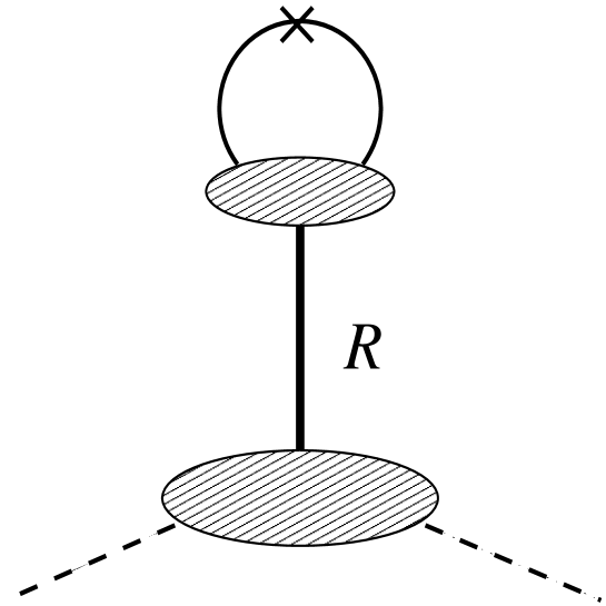
Figure 2: Schematic representation of resonance exchange contributions to the non-forward matrix element of the twist–2 operator in the pion, Eq.(6). The upper blob denotes the distribution amplitude of the spin–$J$ resonance, Eq.(B.2).

Figure 3: Diagrams in the effective low–energy theory contributing to the skewed quark distribution at a low normalization point. The dashed line denotes the pion field, the solid line the quark propagator with the dynamical quark mass, $[i\partial/\hskip 1.49994pt-MF^{2}(\partial^{2})]^{-1}$, and the filled circles the quark–pion vertices contained in the effective action, Eqs.(51) and (52), which include a form factor $F(\partial^{2})$ for each quark line. Diagram (a) contributes only to the isoscalar distribution, and vanishes in the forward limit ($r\rightarrow 0$).

Figure 4: The contributions from diagrams (a) and (b) (cf. Fig.3) to the isoscalar skewed quark distribution in the pion, $H^{I=0}(X,\xi)$, at a low normalization point, as functions of $X$, for a value of $\xi=1$. (Here $t=0$). Dashed lines: Results obtained neglecting the momentum dependence of the dynamical quark mass, cf.  Eqs.(60) and (61). Solid lines: The corresponding contributions obtained when including the form factors, $F(\partial^{2})$. Note that the contribution from diagram (a) is non-zero only in the region $-\xi/2<X<\xi/2$. The momentum dependence of the dynamical quark mass forces this contribution to vanish at the end points, $X=\pm\xi/2$.

Figure 5: The total isoscalar skewed quark distribution in the pion, $H^{I=0}(X,\xi)$, for $\xi=1$, being the sum of the two contributions (a) and (b) shown in Fig.4. Dashed line: Result obtained neglecting the momentum dependence of the dynamical quark mass, cf. Eq.(62). Solid lines: Distribution obtained when including the form factors, $F(\partial^{2})$. Due to the vanishing of contribution (a) at $X=\pm\xi/2$ the total distribution is continuous at these points.

References

- [1] J.C. Collins, L. Frankfurt and M. Strikman, Phys. Rev. D 56, 2982 (1997).
- [2] X.–D. Ji, Phys. Rev. Lett. 78, 610 (1997).
- [3] X.–D. Ji, Phys. Rev. D 55, 7114 (1997).
- [4] A.V. Radyushkin, Phys. Rev. D 56, 5524 (1997).
- [5] A.V. Radyushkin, Phys. Rev. D 59, 014030 (1999).
- [6] X.–D. Ji, and J. Osborne, Phys. Rev. D 57, 1337 (1998); ibid. D 58, 094018 (1998).
- [7] J.C. Collins and A. Freund, Preprint PSU-TH-192, hep-ph/9801262.
- [8] For a review, see: P.A.M. Guichon and M. Vanderhaeghen, Prog. Part. Nucl. Phys. 41, 125 (1998).
- [9] J. Bartels and M. Loewe, Z. Phys. C 12, 263 (1982).
-
[10]
B. Geyer, D. Robaschik, M. Bordag, J. Horejsi
Z. Phys. C 26, 591 (1985);
F.M. Dittes, D. Müller, D. Robaschik, B. Geyer, J. Horejsi Phys. Lett. B 209, 325 (1988). - [11] L.L. Frankfurt, M.V. Polyakov, and M. Strikman, Contribution to Workshop on Jefferson Lab Physics and Instrumentation with 6–12–GeV Beams and Beyond, Newport News, VA, Jun 15–18, 1998; Preprint RUB-TPII-12-98, hep-ph/9808449.
- [12] V.Yu. Petrov, P.V. Pobylitsa, M.V. Polyakov, I. Börnig, K. Goeke, and C. Weiss, Phys. Rev. D 57, 4325 (1998).
- [13] D. Diakonov and V. Petrov, Nucl. Phys. B 272 (1986) 457; LNPI preprint LNPI-1153 (1986), published (in Russian) in: Hadron matter under extreme conditions, Naukova Dumka, Kiev (1986), p.192.
- [14] D.I. Diakonov, V.Yu. Petrov, P.V. Pobylitsa, M.V. Polyakov and C. Weiss, Nucl. Phys. B 480, 341 (1996); Phys. Rev. D 56, 4069 (1997).
- [15] V.Yu. Petrov and P.V. Pobylitsa, hep-ph/9712203.
- [16] V.Yu. Petrov, M.V. Polyakov, R. Ruskov, C. Weiss and K. Goeke, Bochum University preprint hep-ph/9807229; to appear in Phys. Rev. D.
- [17] M. Diehl, T. Gousset, B. Pire and O. Teryaev, Phys. Rev. Lett. 81, 1782 (1998).
- [18] M.V. Polyakov and C. Weiss, Bochum University Preprint RUB-TPII-7/98, hep-ph/9806390, Phys. Rev. D, in press.
- [19] M.V. Polyakov, Preprint RUB-TPII-14/98, hep-ph/9809483.
- [20] The CLEO Collaboration (J. Gronberg et al.), Phys. Rev. D57, 33 (1998).
- [21] G.P. Lepage and S.J. Brodsky, Phys. Lett. B 87, 359 (1979); A.V. Efremov and A.V. Radyushkin, Phys. Lett. B 94, 245 (1980).
- [22] L. Frankfurt, A. Freund, V. Guzey, and M. Strikman, Phys. Lett. B 418, 345 (1998); Erratum ibid. B 429, 414 (1998).
-
[23]
A.V. Belitsky, B. Geyer, D. Müller,
A. Schäfer, Phys. Lett. B 421, 312 (1998);
A.V. Belitsky, D. Müller, L. Niedermeier and A. Schäfer, Phys. Lett. B 437, 160 (1998). - [24] J. Blümlein, B. Geyer and D. Robaschik, Phys. Lett. B 406, 161 (1997).
- [25] L. Mankiewicz, G. Piller and T. Weigl, Eur. Phys. J. C 5, 119 (1998).
- [26] A.V. Radyushkin, Preprint JLAB-THY-98-41 (1998), hep-ph/9810466.
- [27] X.–D. Ji, J. Phys. G 24, 1181 (1998).
- [28] D.I. Diakonov, V.Yu. Petrov, and P.V. Pobylitsa, Nucl. Phys. B 306, 809 (1988).
- [29] A.E. Dorokhov and L. Tomio, Preprint JINR-94-36, hep-ph/9803329.
- [30] M.V. Polyakov, Talk given at conference “Particle and Nuclear Physics with CEBAF at Jefferson Lab”, Dubrovnik, Nov. 3–10, 1998, Bochum Preprint RUB-TPII-02/99, hep-ph/9901315.
- [31] M. Glück, E. Reya, and A. Vogt, Z. Phys. C 53, 651 (1992).
- [32] A.V. Belitsky, Phys. Lett. B 386, 359 (1996).
- [33] P. Ball and V.M. Braun, Phys. Rev. D 54, 2182 (1996).
- [34] A.P. Bakulev and S.V. Mikhailov, Phys. Lett. B 436, 351 (1998).
- [35] V.M. Braun and I.E. Filyanov, Z. Phys. C 44, 157 (1989).
- [36] S.V. Mikhailov and A.V. Radyushkin, Phys. Rev. D 45, 1754 (1992).
- [37] A.P. Bakulev and S.V. Mikhailov, Z. Phys. C 68, 451 (1995).
-
[38]
J. Sakurai, Ann. Phys. (N.Y.) 11, 1 (1960);
G.E. Brown, Mannque Rho and W. Weise, Nucl. Phys. A 454, 669 (1986).