Flux-Tube Ring and Glueball Properties
in the Dual Ginzburg-Landau Theory

Abstract

An intuitive approach to the glueball using the flux-tube ring solution in the dual Ginzburg-Landau theory is presented. The description of the flux-tube ring as the relativistic closed string with the effective string tension enables us to write the hamiltonian of the flux-tube ring using the Nambu-Goto action. Analyzing the Schr$\ddot{\rm{o}}$dinger equation, we discuss the mass spectrum and the wave function of the glueball. The lowest glueball state is found to have the mass $M_{G}\sim 1.6\;{\rm GeV}$ and the size $R_{G}\sim 0.5\;{\rm fm}$.

I Introduction

The existence of glueball states is naively expected in terms of the gluon self-coupling in QCD[1]. Recent progress of lattice QCD simulations predicts the masses of glueballs $M(0^{++})$ = 1.50 $\sim$ 1.75 GeV, $M(2^{++})$ = 2.15 $\sim$ 2.45 GeV [2, 3, 4, 5, 6]. Experimentally, there are some candidates; $f_{0}(1500)$ and $f_{0}(1710)$ for the scalar glueball, $f_{J}(2220)$ ($J$=2 or 4), $f_{2}(2300)$ and $f_{2}(2340)$ for the tensor glueball[7]. However, the abundance of $q$-$\bar{q}$ meson states in the 1 $\sim$ 3 GeV region and the possibility of the quarkonium-glueball mixing states still make it difficult to identify the glueball states[8]. To date, no glueball state has been firmly discovered yet. More studies for the glueballs from many directions are necessary to specify the glueball states.

In this paper, we present an analytic and very intuitive approach to the glueball using the dual Ginzburg-Landau (DGL) theory, an effective theory of the nonperturbative QCD. The DGL theory is constructed from QCD by performing the ’t Hooft abelian projection[9] with the two hypotheses, abelian dominance and monopole condensation[10]. Abelian projection reduces QCD into the ${\rm U(1)^{2}}$ abelian gauge theory including monopoles, and recent studies of the lattice QCD in the maximally abelian (MA) gauge give numerical evidences of QCD-monopole condensation[11, 12] and abelian dominance[13, 14] for the nonperturbative phenomena such as confinement[15, 16], chiral symmetry breaking[17, 18]. In the DGL theory, the QCD-vacuum is described as the dual version of the superconductor and the color confinement is realized by the formation of the color-electric flux-tube through the dual Meissner effect[19, 20, 21, 22]. The flux-tube has a constant energy per unit length, the string tension, which characterizes the strength of the color confinement as the slope of the linear potential between the color charges. The flux-tube solution in the DGL theory appears as the topological excitation as the relevant collective mode in the QCD-vacuum, and this provides intuitive pictures of the hadrons in terms of the string-like structure of the color-electric flux. While the hadrons including the valence quarks correspond to an open flux-tube excitation with terminals, the glueball can be regarded as the flux-tube without end, the “flux-tube ring” excitation[23], in the flux-tube picture[24]. This simple picture is expected to provide the further understanding of the glueball.

In this paper, we consider the simplest ring solution that the ends of the flux-tube meet each other to form a circle. We study then the profiles of the color-electric field and the monopole field with the DGL theory. We calculate also the “effective string tension”, which is the string tension of the flux-tube forming a ring as a function of the ring radius $R$. The flux-tube ring solution in the DGL theory itself is unstable and prefers to shrink, since it does not contain any kinetic term for the ring motion. From the quantum mechanical point of view, such a collapse is to be forbidden by the uncertainty principle. Let us imagine the hydrogen atom, where the stable ground state is determined by the energy balance between the kinetic term of the electron $p^{2}/2m_{e}$ and the Coulomb potential term $-e^{2}/r$ with the uncertainty relation $p\cdot r\geq 1$. Similarly, it would be necessary to introduce the kinetic term of the ring, and take the quantum effect into account. However, it is a difficult problem since we have no guiding principle to determine the kinetic term of the flux-tube. Therefore, in this paper, we introduce the kinetic term based on the string-like description of the flux-tube by using the Nambu-Goto (NG) action in the string theory[25] and we use the principle that the string action is proportional to the world surface swept over the string motion. In this scheme, the flux-tube ring is regarded as the relativistic closed string with the effective string tension, which is calculated based on the DGL theory.

In section II, we investigate the single flux-tube solution in the DGL theory and consider the essence of the flux-tube. The DGL parameters are determined so as to reproduce the string tension $\sigma\simeq 1\;{\rm GeV/fm}$ extracted from the Regge slope of the hadrons[26].

In section III, we study the flux-tube ring solution as the glueball excitation. We investigate the profiles and the effective string tension of the flux-tube ring, and then, we combine the DGL theory with the string theory in order to introduce the kinetic term and write the hamiltonian of the flux-tube ring. Finally, we estimate the mass and the size of the glueball by solving the Schr$\ddot{\rm o}$dinger equation.

Section IV is devoted to the summary of the present study and the discussion.

II Single Flux-Tube Solution in the DGL theory

In this section, we consider the topological solution related to the $q$-$\bar{q}$ system in the dual Ginzburg-Landau (DGL) theory within the quenched level. The system is described by the DGL lagrangian[19, 20],

$${\cal L}_{\rm DGL}=-\frac{1}{4}\left(\partial_{\mu}\vec{B}_{\nu}-\partial_{\nu}\vec{B}_{\mu}-\frac{1}{n\cdot\partial}\varepsilon_{\mu\nu\alpha\beta}n^{\alpha}\vec{j}^{\beta}\right)^{2}+\sum_{\alpha=1}^{3}\left[\left|\left(\partial_{\mu}+ig\vec{\epsilon}_{\alpha}{\cdot}\vec{B}_{\mu}\right)\chi_{\alpha}\right|^{2}-\lambda\left(\left|\chi_{\alpha}\right|^{2}-v^{2}\right)^{2}\right],$$ (1)

where $\vec{B}_{\mu}$ and $\chi_{\alpha}$ denote the dual gauge field with two components $(B_{\mu}^{3},B_{\mu}^{8})$ and the complex scalar monopole field, respectively. Here, $\vec{\epsilon}_{a}$ is the root vector of SU(3) algebra, $\vec{\epsilon}_{1}=\left(-1/2,\sqrt{3}/2\right),\vec{\epsilon}_{2}=\left(-1/2,-\sqrt{3}/2\right),\vec{\epsilon}_{3}=\left(1,0\right)$, and $n^{\mu}$ denotes an arbitrary constant 4-vector, which corresponds to the direction of the Dirac string. At the quenched level, the color sources are given as the $c$-number current, and the heavy $q$-$\bar{q}$ system provides

$${\vec{j}^{\mu}}_{\alpha}(x)\equiv\vec{Q}_{\alpha}g^{\mu 0}\left[\delta^{3}\left(\mbox{\boldmath$x$}-\mbox{\boldmath$a$}\right)-\delta^{3}\left(\mbox{\boldmath$x$}-\mbox{\boldmath$b$}\right)\right],$$ (2)

where $\vec{Q}_{\alpha}\equiv e\vec{w}_{\alpha}$ is the abelian color-electric charge of the quark. Here, $a$ and $b$ are position vectors of the quark and the antiquark, respectively, and $w_{\alpha}$ is the weight vector of SU(3) algebra, $\vec{w}_{1}=\left(1/2,\sqrt{3}/6\right),\vec{w}_{2}=\left(-1/2,\sqrt{3}/6\right),\vec{w}_{3}=\left(0,-1/\sqrt{3}\right)$. The label $\alpha=1,2,3$ corresponds to the color-electric charge, red(R), blue(B) and green(G). According to the Gauss law, one finds the color-electric field and then the dual gauge field $\vec{B}_{\mu}$ is proportional to the quark charge $\vec{Q}_{\alpha}$[21, 22]. For instance, when we consider the ${\rm R}$-$\bar{\rm{R}}$ system, the dual gauge field can be defined by using the weight vector as $\vec{B}_{\mu}\equiv\vec{w}_{1}B_{\mu}^{\rm R}$. In this system, the DGL lagrangian (1) can be written as

$${\cal L^{\prime}}_{\rm DGL} = -\frac{1}{3}\cdot\frac{1}{4}\left(\partial_{\mu}B_{\nu}^{\rm R}-\partial_{\nu}B_{\mu}^{\rm R}\right)^{2}+\left|\partial_{\mu}\chi_{1}\right|^{2}-\lambda\left(\left|\chi_{1}\right|^{2}-v^{2}\right)^{2}$$ (5)

$$+\left|\left(\partial_{\mu}-\frac{1}{2}igB_{\mu}^{\rm R}\right)\chi_{2}\right|^{2}-\lambda\left(\left|\chi_{2}\right|^{2}-v^{2}\right)^{2}$$

$$+\left|\left(\partial_{\mu}+\frac{1}{2}igB_{\mu}^{\rm R}\right)\chi_{3}\right|^{2}-\lambda\left(\left|\chi_{3}\right|^{2}-v^{2}\right)^{2},$$

where we use the relation, $\vec{\epsilon}_{\alpha}\cdot\vec{B}_{\mu}=\vec{\epsilon}_{\alpha}\cdot\vec{w}_{1}B_{\mu}^{\rm R}=\frac{1}{2}\;\left(\;0,-1,1\;\right)\;B_{\mu}^{\rm R}$. By considering the constraint condition of the phase of the monopole field $\sum_{\alpha=1}^{3}arg\;\chi_{\alpha}$=0[19, 20], we can write the monopole field, in this case, as $\chi_{1}=v$, $\chi_{2}={\chi^{\rm R}}^{\ast}$, $\chi_{3}=\chi^{\rm R}$. The DGL lagrangian (5) is then given by

$${\cal L^{\prime}}_{\rm DGL} = -\frac{1}{3}\cdot\frac{1}{4}\left(\partial_{\mu}B_{\nu}^{\rm R}-\partial_{\nu}B_{\mu}^{\rm R}\right)^{2}$$ (7)

$$+2\left|\left(\partial_{\mu}+\frac{1}{2}igB_{\mu}^{\rm R}\right)\chi^{\rm R}\right|^{2}-2\lambda\left(\left|\chi^{\rm R}\right|^{2}-v^{2}\right)^{2}.$$

With the redefinitions of the fields and the parameters,

$$B_{\mu}^{\rm R}\equiv\sqrt{3}B_{\mu},\quad\chi^{\rm R}\equiv\chi,\quad g\equiv\frac{2}{\sqrt{3}}\hat{g},\quad\lambda\equiv 2\hat{\lambda},\quad v\equiv\frac{1}{\sqrt{2}}\hat{v},$$ (8)

we get the final expression for the ${\rm R}$-$\bar{\rm{R}}$ system,

$${\cal L^{\prime}}_{\rm DGL}=-\frac{1}{4}\left(\partial_{\mu}B_{\nu}-\partial_{\nu}B_{\mu}\right)^{2}+\left|\left(\partial_{\mu}+i\hat{g}B_{\mu}\right)\chi\right|^{2}-\hat{\lambda}\left(\left|\chi\right|^{2}-\hat{v}^{2}\right)^{2}.$$ (9)

For the other two color-singlet cases such as the ${\rm B}$-$\bar{\rm{B}}$ and the ${\rm G}$-$\bar{\rm{G}}$ system, one obtains the same expression owing to the Weyl symmetry among three color charges, ${\rm R}$, ${\rm B}$ and ${\rm G}$. The lagrangian (9) has the U(1) gauge symmetry and its form coincides with the Ginzburg-Landau theory for superconductivity. This type of lagrangian has the flux-tube solution such as the Abrikosov vortex[27].

To see this solution, we consider the field equations,

$$(\partial_{\mu}+i\hat{g}B_{\mu})^{2}\chi=2\hat{\lambda}\chi(\hat{v}^{2}-\chi^{*}\chi),$$ (10)

$$\partial^{\nu}{}^{*}F_{\mu\nu}\equiv k_{\mu}=-i\hat{g}(\chi^{*}\partial_{\mu}\chi-\chi\partial_{\mu}\chi^{*})+2\hat{g}^{2}B_{\mu}\chi^{*}\chi,$$ (11)

$${}^{*}F_{\mu\nu}\equiv\partial_{\mu}B_{\nu}-\partial_{\nu}B_{\mu},$$ (12)

with the proper boundary conditions that quantize the color-electric flux. The flux is given by

$$\Phi\equiv\int{}^{*}F_{\mu\nu}d\sigma^{\mu\nu}=\oint B_{\mu}(x)dx^{\mu},$$ (13)

where $\sigma^{\mu\nu}$ is a two-dimensional surface element in the Minkowski space. By the polar decomposition of the monopole field using two scalar variables, $\phi$ and $f$ as $\chi(x)=\phi(x)e^{if(x)}$, we obtain from Eq.(11)

$$B_{\mu}=\frac{1}{2\hat{g}^{2}}\frac{k_{\mu}}{\phi^{2}}-\frac{1}{\hat{g}}\partial_{\mu}f.$$ (14)

We substitute this expression into (13) and integrate out over a large closed loop where the current $k_{\mu}$ is vanished. Thus we get

$$\Phi=-\frac{1}{\hat{g}}\oint\partial_{\mu}f(x)dx^{\mu}.$$ (15)

Since the only requirement on the phase $f(x)$ is that $\chi(x)$ should be a single valued, the line integral (15) does not necessarily vanish. It means that $f(x)$ can be varied by $2\pi n$ ($n$=integer), therefore

$$\Phi=-\frac{2\pi n}{\hat{g}},$$ (16)

and the flux is quantized as a result of this condition. Integer $n$ is regarded as the winding number of the flux-tube corresponding to the topological charge.

Let us consider the single flux-tube solution with translational invariance (it also has cylindrical symmetry) along the $z$-axis, which is expected to appear in the $q$-$\bar{q}$ system. In such a system, the dual gauge field and the monopole field can be written using the radial coordinate $r$ as

$$B = B(r)\mbox{\boldmath$e$}_{\theta}=\frac{\tilde{B}(r)}{r}\mbox{\boldmath$e$}_{\theta},$$ (17)

$$\phi = \phi(r),$$ (18)

and the phase is $f=n\theta$, where $\theta$ is the azimuth around the $z$-axis. The differential of the phase is $\nabla f=(n/r)\;\mbox{\boldmath$e$}_{\theta}$ and its integration over a closed loop leads the flux quantization condition (16). The color-electric field is defined by the rotation of the dual gauge field,

$$\mbox{\boldmath$E$}\equiv\nabla\times\mbox{\boldmath$B$}=\frac{1}{r}\frac{d\tilde{B}(r)}{dr}\mbox{\boldmath$e$}_{z}\equiv E_{z}(r)\mbox{\boldmath$e$}_{z},$$ (19)

where $\mbox{\boldmath$e$}_{z}$ is a unit vector along the $z$-axis. The field equations (10) and (11) are given by,

$$\frac{d^{2}\phi}{dr^{2}}+\frac{1}{r}\frac{d\phi}{dr}-\left(\frac{n-\hat{g}\tilde{B}}{r}\right)^{2}\phi-2\hat{\lambda}\phi\;(\phi^{2}-\hat{v}^{2})=0,$$ (20)

$$\frac{d^{2}\tilde{B}}{dr^{2}}-\frac{1}{r}\frac{d\tilde{B}}{dr}+2\hat{g}\;(n-\hat{g}\tilde{B})\phi^{2}=0,$$ (21)

and the energy of the flux-tube per unit length $1/\hat{v}$ along the $z$-axis is obtained as

$$E_{n}=\frac{2\pi}{\hat{v}}\int_{0}^{\infty}rdr\left[\frac{1}{2}\left(\frac{1}{r}\frac{d\tilde{B}}{dr}\right)^{2}+\left(\frac{d\phi}{dr}\right)^{2}+\left(\frac{n-\hat{g}\tilde{B}}{r}\right)^{2}\phi^{2}+\hat{\lambda}(\phi^{2}-\hat{v}^{2})^{2}\right].$$ (22)

Since the flux-tube solution should give a finite energy, one finds the boundary conditions,

$$\tilde{B}(r)=0,\quad\phi(r)=0\quad{\rm as}\quad r\to 0,$$ (23)

$$\tilde{B}(r)=\frac{n}{\hat{g}},\quad\phi(r)=\hat{v}\quad{\rm as}\quad r\to\infty.$$ (24)

The string tension can be defined by using the expression of the energy (22) as

$$\sigma\equiv\frac{E_{n=1}}{\int_{0}^{1/\hat{v}}dz}=E_{n=1}\hat{v}.$$ (25)

In Fig.1, we show the numerical solution of the flux-tube, the profiles of the color-electric field $E_{z}(r)$ and the monopole field $\phi(r)$ with the winding number $n$=1, where the parameters are fixed as

$$\hat{g}=2.6,\quad\hat{\lambda}=33,\quad\hat{v}=0.14\;{\rm GeV},$$ (26)

or equivalently, $g=2.9$, $e=4\pi/g=4.3$, $\lambda=66$, $v=0.098\;{\rm GeV}$ (see (8)). These parameters reproduce the string tension $\sigma=1.0\;{\rm GeV/fm}$ and two characteristic mass scales which are presented by $m_{\chi}\equiv 2\sqrt{\hat{\lambda}}\hat{v}$ and $m_{B}\equiv\sqrt{2}\hat{g}\hat{v}$ as $m_{\chi}=1.6\;{\rm GeV}$ and $m_{B}=0.5\;{\rm GeV}$, respectively. The $m_{\chi}$ denotes the monopole mass, which is the threshold energy to excite the monopole in the QCD-vacuum corresponding to the Bogoliubov particle so-called “Bogoliubon” in the ordinary superconductor[28]. If such excitations dominate, the phase transition is expected to occur and this value $m_{\chi}$ is regarded as the ultra-violet cutoff of the DGL theory. The $m_{B}$ is the dual gauge mass, which determines the magnitude of the dual Meissner effect. The value 0.5 GeV is supported by the recent calculation based on the lattice QCD using the dual formalism[12]. These inverse masses $m_{\chi}^{-1}$= 0.12 fm and $m_{B}^{-1}$= 0.39 fm are regarded as the coherent length of the monopole field and the penetration depth of the color-electric field, respectively. The ratio of these two lengths gives the Ginzburg-Landau (GL) parameter,

$$\tilde{\kappa}\equiv\frac{m_{B}^{-1}}{m_{\chi}^{-1}}=\frac{\sqrt{2\hat{\lambda}}}{\hat{g}}.$$ (27)

The GL-parameter plays an important role to define the vacuum properties, where $\tilde{\kappa}<1$ describes the type-I vacuum and $\tilde{\kappa}>1$ is the type-II vacuum. The parameters (26) lead the GL-parameter as $\tilde{\kappa}=3.0>1$, which indicates that the QCD-vacuum belongs to the type-II vacuum[29].

In such a type-II vacuum, one can treat the field equations (20) and (21) analytically within the mean field approximation $\phi\sim\hat{v}$ with the cutoff $m_{B}=m_{B}\;\theta(r-m_{\chi}^{-1})$. The cutoff is necessary in order to avoid the unphysical divergence at the core of the flux-tube. The mean field approximation leads the dual London equation from Eq.(21),

$$\frac{d^{2}\tilde{B}}{dr^{2}}-\frac{1}{r}\frac{d\tilde{B}}{dr}+2\hat{g}(n-\hat{g}\tilde{B})\hat{v}^{2}=0,$$ (28)

and the replacements $r\equiv m_{B}^{-1}\rho$ and $\tilde{B}(\rho)\equiv n/\hat{g}-\rho K(\rho)$ give

$$\frac{d^{2}K}{d\rho^{2}}+\frac{1}{\rho}\frac{dK}{d\rho}-\left(1+\frac{1}{\rho^{2}}\right)K=0.$$ (29)

We know this solution is described by the first order modified Bessel function $K_{1}(\rho)$, which asymptotically behaves as $K_{1}(\rho)\sim\sqrt{\frac{\pi}{2\rho}}e^{-\rho}$. Thus one obtains the profiles of the dual gauge field and the color-electric field,

$$\tilde{B}(\rho)\sim\frac{n}{\hat{g}}-\rho\sqrt{\frac{\pi}{2\rho}}e^{-\rho},\quad\quad E_{z}(\rho)\sim\sqrt{\frac{\pi}{2\rho}}e^{-\rho}.$$ (30)

The color-electric field is excluded from the vacuum and hence confined inside the region $\rho<1$ ($r<m_{B}^{-1}$), which means the vortex-type, i.e. the flux-tube configuration. Of course, these expressions are valid for the outside region of the cutoff $r>m_{\chi}^{-1}$. If we want to get the whole region of the profiles with the arbitrary parameters, we must resort to the numerical calculations as shown in Fig.1. In any case, the DGL theory explains the formation of the flux-tube in the QCD-vacuum, which provides the linear confinement potential between the quark and the antiquark.

Here we shall discuss some important features of the flux-tube. As we can confirm, the phase of the monopole field $f=n\theta$ leads the differential form of the flux quantization condition,

$$\nabla\times\nabla f=2\pi n\delta(x)\delta(y)\mbox{\boldmath$e$}_{z},$$ (31)

where the delta functions characterize the center of the flux-tube. Thus, an essential point for the formation of the flux-tube is that the phase of the monopole field becomes singular at the center of the color-electric flux. That is to say, if we want to obtain the flux-tube solution, all we have to do is to impose the singular structure on the phase. We also find that the setting of the phase provides the boundary condition of the dual gauge field uniquely as is presented in Eq.(14) that the dual gauge field should behave as $B_{\mu}\to-\frac{1}{\hat{g}}\partial_{\mu}f$ at the current $k_{\mu}\simeq 0$.

III Glueball as the Flux-Tube Ring Solution

In this section, we consider the flux-tube ring solution that the ends of the flux-tube meet each other to form a circle with the radius $R$ as shown in Fig.2. The singular structure on the phase of the monopole field is characterized by the rotational invariance along the $z$-axis,

$$\nabla\times\nabla f=2\pi n\;\delta(r-R)\;\delta(z)\mbox{\boldmath$e$}_{\theta},$$ (32)

where $n$ is the winding number of the flux-tube composing the ring. The fields can be written as

$$B = B_{r}(r,z)\mbox{\boldmath$e$}_{r}+B_{z}(r,z)\mbox{\boldmath$e$}_{z},$$ (33)

$$\phi = \phi(r,z),$$ (34)

and the phase is determined by Eq.(32) as $f=-n\;\tan^{-1}\left(z/(r-R)\right)$. The factor minus comes from the use of the cylindrical coordinate. The field equations are obtained by substituting these expressions into Eqs.(10) and (11),

$$\frac{\partial^{2}\phi}{\partial r^{2}}+\frac{\partial^{2}\phi}{\partial z^{2}}+\frac{1}{r}\frac{\partial\phi}{\partial r}-\hat{g}^{2}\left({B^{\prime}_{r}}^{2}+{B^{\prime}_{z}}^{2}\right)\phi-2\hat{\lambda}\;\phi\;(\phi^{2}-\hat{v}^{2})=0,$$ (35)

$$\frac{\partial^{2}B_{z}}{\partial z\partial r}-\frac{\partial^{2}B_{r}}{\partial z^{2}}+2\hat{g}^{2}B^{\prime}_{r}\phi^{2}=0,$$ (36)

$$\frac{\partial^{2}B_{r}}{\partial r\partial z}-\frac{\partial^{2}B_{z}}{\partial r^{2}}+\frac{1}{r}\left(\frac{\partial B_{r}}{\partial z}-\frac{\partial B_{z}}{\partial r}\right)+2\hat{g}^{2}B^{\prime}_{z}\phi^{2}=0,$$ (37)

with

$$B^{\prime}_{r} \equiv B_{r}-\frac{\partial f}{\partial r}=B_{r}-n\frac{z}{(r-R)^{2}+z^{2}},$$ (38)

$$B^{\prime}_{z} \equiv B_{z}-\frac{\partial f}{\partial z}=B_{z}+n\frac{r-R}{(r-R)^{2}+z^{2}}.$$ (39)

The boundary conditions are given by

$$\phi(r,z)=0\quad{\rm as}\quad(r,z)\to(R,0),$$ (40)

$$B^{\prime}_{r}(r,z)=0,\quad B^{\prime}_{z}(r,z)=0\quad{\rm and}\quad\phi(r,z)=\hat{v}\quad{\rm as}\quad\sqrt{(r-R)^{2}+z^{2}}\to\infty.$$ (41)

For $r\to 0$, the color-electric field is required to disappear due to the rotational symmetry around the $z$-axis.

In Figs. 3 and 4, we show the numerical solutions of the profiles of the color-electric field and the monopole field as a function of the ring radius $R$. These profiles show the tendencies of shrinking of the color-electric field and the monopole field as the ring radius $R$ is reduced. Accordingly, we also obtain the effective string tension $\sigma_{\rm eff}(R)$ as a function of the ring radius as shown in Fig.5. $\sigma_{\rm eff}(R)$ is defined by

$$E(R)=2\pi R\sigma_{\rm eff}(R),$$ (42)

where $E(R)$ is the energy of the flux-tube ring,

$$E(R)\!=\!2\pi\!\!\int_{0}^{\infty}\!\!\!\!\!\!rdr\!\!\int_{-\infty}^{\infty}\!\!\!\!\!\!\!dz\!\left[\frac{1}{2}\left(\frac{\partial B_{r}}{\partial z}\!-\!\frac{\partial B_{z}}{\partial r}\right)^{2}\!\!\!\!+\!\!\left(\frac{\partial\phi}{\partial r}\right)^{2}\!\!\!\!+\!\!\left(\frac{\partial\phi}{\partial z}\right)^{2}\!\!\!\!+\!\hat{g}^{2}({B^{\prime}_{r}}^{2}\!\!+\!{B^{\prime}_{z}}^{2})\phi^{2}\!+\!\hat{\lambda}(\phi^{2}\!-\!\hat{v}^{2})^{2}\right].$$ (43)

We find the string tension is effectively reduced with decreasing the ring radius $R$, which is considered to be caused by the reduction of the color-electric field. The energy $E(R)$ decreases as the ring radius $R$ is reduced. That is to say, the flux-tube ring solution in the DGL theory itself is unstable and prefers to shrink, since it does not contain any kinetic term for the ring motion.

From the quantum mechanical point of view, such a collapse is to be forbidden by the uncertainty principle like the hydrogen atom, where the kinetic term of the electron plays an important role for the stability of the atom. Hence, in order to get the stable ring solution for its motion, it would be necessary to introduce the kinetic term of the ring. Since the flux-tube is characterized by the string-like singular structure on the phase of the monopole field, it seems reasonable to describe the flux-tube ring as the relativistic closed string with the effective string tension $\sigma_{\rm eff}(R)$ by using the Nambu-Goto (NG) action. The description is quite simple. The NG action of the relativistic closed string with the string tension $\Sigma$ is written in general,

$$S=\int_{\tau_{I}}^{\tau_{F}}\!\!\!d\tau\int_{0}^{2\pi}\!\!\!d\theta\;\left[-\Sigma\;\sqrt{(\dot{X}X^{\prime})^{2}-(\dot{X})^{2}(X^{\prime})^{2}}\;\right],$$ (44)

where $X^{\mu}=X^{\mu}(\tau,\theta)$ denotes the string world sheet, $\dot{X}^{\mu}\equiv\partial X^{\mu}/\partial\tau$ and ${X^{\mu}}^{\prime}\equiv\partial X^{\mu}/\partial\theta$.

We parameterize the ring as a circle with the radius $R$,

$$X^{1}(\tau,\theta)=R(\tau)\cos\theta,\quad X^{2}(\tau,\theta)=R(\tau)\sin\theta,$$ (45)

and choose the chronological gauge $X^{0}(\tau,\theta)\equiv\tau$. This parameterization satisfies the orthogonal condition $\dot{\mbox{\boldmath$X$}}\cdot\mbox{\boldmath$X$}^{\prime}=0$. Thus, we obtain the action of the flux-tube ring,

$$S_{\rm ring}=\int_{\tau_{I}}^{\tau_{F}}\!\!\!d\tau\int_{0}^{2\pi}\!\!\!d\theta\;\left[-\sigma_{\rm eff}(R)R\sqrt{1-\dot{R}^{2}}\;\right],$$ (46)

and the hamiltonian of the ring,

$$H(P_{R},R)=\sqrt{P_{R}^{2}+\{2\pi R\sigma_{\rm eff}(R)\}^{2}},$$ (47)

where $P_{R}$ is the canonical conjugate momentum of the coordinate $R$, defined by

$$P_{R}\equiv 2\pi R\sigma_{\rm eff}(R)\frac{\dot{R}}{\sqrt{1-\dot{R}^{2}}}.$$ (48)

If we put $P_{R}=0$ ($\dot{R}=0$), the hamiltonian provides the static energy (42).

Once the ring hamiltonian including the kinetic term is obtained, we can look for the glueball states by solving the Schr$\ddot{\rm o}$dinger equation

$$\left[-\frac{d^{2}}{dR^{2}}+\{2\pi R\sigma_{\rm eff}(R)\}^{2}\right]\;\Phi_{m}(R)={M_{m}}^{2}\;\Phi_{m}(R),$$ (49)

with the boundary conditions,

$$\Phi_{m}(R=0)=0,\quad\Phi_{m}(R=\infty)=0.$$ (50)

The boundary condition $\Phi_{m}(0)$=0 is required in terms of the ring structure of the flux-tube since the wave function is considered to characterize the configuration of the color-electric flux.

It is useful to consider the type-II limit where the effective string tension has a constant value; $\sigma_{\rm eff}(R)\approx\sigma$ ($\simeq$ 1.0 GeV/fm). In this case, the ring hamiltonian reduces into the harmonic-oscillator in one dimension and we can easily obtain the analytic form of the wave function and the mass spectrum,

$$\Phi_{m}(R)\propto H_{m}(\sqrt{2\pi\sigma}R)\exp(-\pi\sigma R^{2}),$$ (51)

$$M_{m}=\sqrt{4\pi\sigma\left(m+\frac{1}{2}\right)},$$ (52)

where $H_{m}(x)$ is Hermite polynomials, $H_{0}(x)=1$, $H_{1}(x)=x$ and so on. One finds the state $m=1,3,5,\cdots$ satisfy the boundary condition $\Phi_{m}(0)$=0. Thus, we get

$$\Phi_{1}(R)=2^{7/2}\pi\sigma^{3/2}R\exp(-\pi\sigma R^{2}),$$ (53)

$$M_{1}=\sqrt{6\pi\sigma}=4.34\sqrt{\sigma}=1.93\;{\rm GeV},$$ (54)

for the lowest state of the flux-tube ring. The root mean square radius is obtained as

$$\sqrt{\langle{R_{1}}^{2}\rangle}\equiv\int_{0}^{\infty}dR\Phi_{1}R^{2}\Phi_{1}=\sqrt{\frac{3}{4\pi\sigma}}=0.489\frac{1}{\sqrt{\sigma}}=0.23\;{\rm fm}.$$ (55)

Let us calculate the ground state of the $m=1$ state for the $\tilde{\kappa}=3.0$ case. In this case, we should resort to the variational method since the effective string tension is not a constant value and is given as the numerical function of the radius $R$. We use the trial function $\Phi_{1}(R,a)\propto R\exp(-a\pi\sigma R^{2})$ where $a$ is the variational parameter determined by minimizing

$$M_{1}(a)\equiv\sqrt{\frac{\langle\Phi_{1}(R,a)|H(P_{R},R)^{2}|\Phi_{1}(R,a)\rangle}{\langle\Phi_{1}(R,a)|\Phi_{1}(R,a)\rangle}},$$ (56)

and we obtain $M_{1}(a=0.82)=1.6\;{\rm GeV}$ as shown in Fig.6, which is regarded as the lowest glueball mass $M_{G}$. As for the root mean square radius, $a=0.82<1$ suggests that the ring radius becomes broad compared with $\sqrt{3/4\pi\sigma}$ for the type-II limit case by the factor $1/\sqrt{a}$. Therefore, we estimate the ring radius as $0.25\;{\rm fm}$ and the size of the glueball as $R_{G}=0.25\times 2=0.5\;{\rm fm}$ (the ring diameter). We find that this mass spectrum $M_{G}$=1.6 GeV is almost consistent with the scalar glueball mass that the lattice QCD predicts for the lowest state[2, 3, 4, 5, 6].

It is interesting to note that the expression (54) is very similar to the following form[30],

$$M(0^{++})=3\sqrt{2}\sqrt{\sigma}\simeq 4.24\sqrt{\sigma},$$ (57)

which is naively derived by the procedure of the minimization of the energy of a bound state of two massless gluons,

$$E=2p+\frac{9}{4}\sigma r-\frac{\alpha}{r},$$ (58)

where $p$ is the gluon momentum and $\alpha$ the strong coupling constant. The color factor 9/4 is given by the ratio of the SU($N_{c}$) Casimir operators of the adjoint representation $N_{c}$ and the fundamental representation $({N_{c}}^{2}-1)/2N_{c}$ for $N_{c}$=3. The uncertainty relation $p\cdot r\geq 1$ leads the energy minimum $E=3\sqrt{(2-\alpha)\sigma}\approx 3\sqrt{2}\sqrt{\sigma}$ at $r=2\sqrt{2-\alpha}/3\sqrt{\sigma}\approx 2\sqrt{2}/3\sqrt{\sigma}=0.943/\sqrt{\sigma}$. One may find that this glueball size 0.943/$\sqrt{\sigma}$ is also consistent with two times of 0.489/$\sqrt{\sigma}$ in (55). These similarities seem to suggest a close relation between the flux-tube ring picture and the phenomenological potential picture of the glueball.

IV Summary and discussions

We have studied the flux-tube ring solution in the dual Ginzburg-Landau (DGL) theory as the glueball excitation. The flux-tube solution in the DGL theory explains the color confinement and also provides intuitive pictures of the hadrons in terms of the string-like structure of the color-electric flux. The hadrons including the valence quarks topologically correspond to the open flux-tube excitation with terminals. Thus, the glueball, which is considered as an object without valence quarks, can be regarded as the flux-tube ring intuitively.

By considering the rotational invariant system along the $z$-axis as shown in Fig.2, we have studied the profiles of the color-electric field and the monopole field as a function of the ring radius. We have used the parameters which reproduce $m_{B}$=0.5 GeV, $m_{\chi}$=1.6 GeV and the string tension $\sigma$=1.0 GeV/fm. The GL-parameter is found to be $\tilde{\kappa}$=3.0, which suggests that the QCD-vacuum belongs to the type-II vacuum. We have calculated the effective string tension $\sigma_{\rm eff}(R)$ as a function of the ring radius. $\sigma_{\rm eff}(R)$ is defined by the relation $E(R)\!=\!2\pi R\sigma_{\rm eff}(R)$, where $E(R)$ is the energy of the ring with the radius $R$. We have found the profiles are reduced with decreasing the ring radius $R$ and accordingly the effective string tension is reduced. These results characterize the size effect of the flux-tube, which is the difference between the flux-tube and the string.

In order to include the kinetic term of the ring, we have described the flux-tube ring as the relativistic closed string with the effective string tension. Using the Nambu-Goto (NG) action, we have parameterized the ring as a circle with the radius $R$ and obtained the hamiltonian $H(P_{R},R)\!=\!\sqrt{P_{R}^{2}+\{2\pi R\sigma_{\rm eff}(R)\}^{2}}$, where $P_{R}$ is the canonical conjugate momentum of the coordinate $R$. If we put $P_{R}=0$, the hamiltonian leads the static energy $E(R)$. Analyzing the Schr$\ddot{\rm o}$dinger equation $H(P_{R},R)^{2}\Phi(R)\!\!=\!\!{M}^{2}\Phi(R)$ with the boundary condition $\Phi(R=0)\!\!=\!\!\Phi(R=\infty)\!\!=\!\!0$, we have obtained the eigenvalue $M_{G}\!=\!\!1.6\;{\rm GeV}$ for the ground state, which is considered as the lowest glueball mass. The size of the glueball is estimated as $R_{G}\!=\!\!0.5\;{\rm fm}$. The mass spectrum $M_{G}\!=\!\!1.6\;{\rm GeV}$ is almost consistent with the scalar glueball mass that the lattice QCD predicts for the lowest state. We have found these results are very similar to another approach based on the Regge phenomenology, where the color factor 9/4 in the linear potential between two gluons plays important roles for the estimation of the glueball mass and the size. These similarities are quite interesting and the phenomenological potential picture of the glueball seems to have a close relation with the flux-tube ring picture.

Here, we shall discuss about the relation between the glueball and the monopole. One may find that the $m_{\chi}$=1.6 GeV is very similar to the glueball mass that we have obtained above analysis. The monopole field denotes a complex scalar field and its origin is the off-diagonal gluon field in the MA-gauge in QCD. Thus, the monopole field would also present the scalar gluonic excitation in the QCD-vacuum such as the scalar glueball[19]. Therefore, this resemblance of masses seems to be quite natural, in fact, the phase of the monopole field has played an essential role for the flux-tube ring solution. It is interesting to note that once this identification is allowed, we can determine the mass $m_{\chi}$ self-consistently. In such a case, the DGL theory which is now including three-parameters can be rewritten to the two-parameters theory. However, whether the both scalar glueballs presented by the flux-tube ring or the monopole field are the same or not is another problem since the flux-tube ring depends not only on the GL-parameter but also on the string tension. We are now investigating the scalar glueball in terms of the monopole field in the DGL theory.

Again, we would like to mention that our main idea is the description of the flux-tube ring solution in the DGL theory as the relativistic closed string with the effective string tension, which enables us to write the hamiltonian of the flux-tube ring using the NG action. Once the hamiltonian is obtained, we can discuss the mass spectrum and the wave function of the glueball state. The boundary condition $\Phi(R=0)$=0 dictates the ring structure of the color-electric flux to the wave function. In the future, we should consider the collective motion of the ring and extract the physical glueball state with definite quantum numbers $J^{PC}$ using the angular momentum projection method. Although such approaches are in progress, we can expect that the DGL theory provides a useful method for the study of the glueball.

Figure Captions

FIG.1 : Profiles of the color-electric field $E_{z}(r)$ (dotted) and the monopole field $\phi(r)$ (solid) of the cylindrical flux-tube in the type-II ($\tilde{\kappa}=3.0$) vacuum as functions of the radial distance from the center of the flux-tube $r$, where the parameters are fixed as $\hat{g}=2.6,\hat{\lambda}=33,\hat{v}=0.14\;{\rm GeV}$.

FIG.2 : The flux-tube ring system which has rotational invariance along the $z$-axis. $R$ denotes the ring radius. All the coordinates used in the text are defined in this figure.

FIG.3 : The profiles of the color-electric field $E_{\theta}(r,z)$ in unit of $1/{\rm fm^{2}}$ of the flux-tube ring system in the type-II ($\tilde{\kappa}=3.0$) vacuum. The left-hand side denotes the 3D plot and the right-hand side is its contour plot. The unit of the radial coordinate $r$ and the $z$-axis is fm. The radius is taken from 2.0 fm (upper) to 0.5 fm (below) in step of 0.5fm. The color-electric field $E_{\theta}$ decreases as the ring radius $R$ is reduced.

FIG.4 : The profiles of the monopole field $\phi(r,z)$ in unit of $1/{\rm fm}$ of the flux-tube ring system in the type-II ($\tilde{\kappa}=3.0$) vacuum. The left-hand side denotes the 3D plot and the right-hand side is its contour plot. The unit of the radial coordinate $r$ and the $z$-axis is fm. The radius is taken from 2.0 fm (upper) to 0.5 fm (below) in step of 0.5fm. The monopole field $\phi$ at the central region of the ring decreases as the ring radius $R$ is reduced.

FIG.5 : Effective string tension $\sigma_{\rm eff}(R)$ in GeV/fm as a function of the ring radius $R$. As the ring radius is reduced, the effective string tension decreases to zero.

FIG.6 : The energy expectation value $M_{1}(a)$ of the flux-tube ring system as a function of the variational parameter $a$. The dotted line denotes the case of the constant string tension $\sigma=1.0\;{\rm GeV/fm}$ (for type-II limit), where the energy minimum shows 1.93 GeV at $a=1$ as we have obtained in the analytical way. The solid line is the main result by using the effective string tension $\sigma_{\rm eff}(R)$ (for $\tilde{\kappa}=3.0$), which shows the energy minimum 1.60 GeV at $a=0.82$. The result $a<1$ suggests that the wave function is broad compared with the type-II limit.

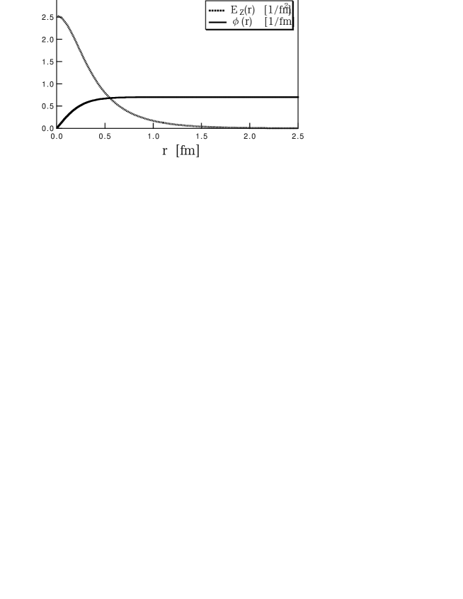
FIG. 1.:

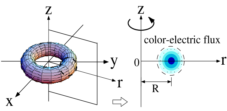
FIG. 2.:

FIG. 3.:

FIG. 4.:

FIG. 5.:

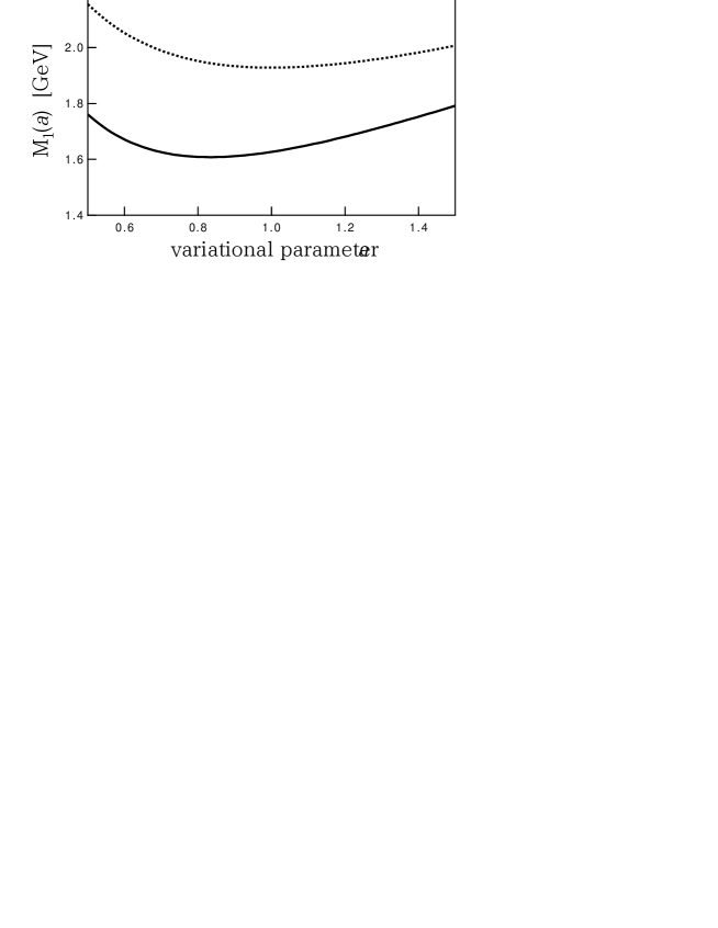
FIG. 6.:

REFERENCES

- [1] M. Creutz, “Quarks, Gluons and Lattice”, (Cambridge, Uk: Univ. Pr. 1983), p.1.
- [2] G. Bali, K. Schilling, A. Hulsebos, A. Irving, C. Michael and P. Stephenson, Phys. Lett. B 309, 378 (1993).
- [3] H. Chen, J. Sexton, A. Vaccarino and D. Weingarten, Nucl. Phys. B (Proc. Suppl.) 34, 357 (1994).
- [4] J. Sexton, A. Vaccarino and D. Weingarten, Phys. Rev. Lett. 75, 4563 (1995); Nucl. Phys. B (Proc. Suppl.) 47, 128 (1996).
- [5] M.J. Teper “Physics from the lattice: glueballs in QCD; topology; SU(N) for all N”, hep-lat/9711011.
- [6] C. Morningstar and M. Peardon, Phys. Rev. D 56, 4043 (1997).
- [7] C. Caso et al. Particle Data Group, Euro. Phys. J. C3, 1 (1998).
- [8] N.A. Trnqvist, in Proceedings of International Europhysics Conference on High Energy Physics (HEP 95), Brussels, Belgium, July 1995, (World Scientific) p.84.
- [9] G. ’t Hooft, Nucl. Phys. B 190, 455 (1981).
- [10] Z.F. Ezawa and A. Iwasaki, Phys. Rev. D 25, 2681 (1982); Phys. Rev. D 26, 631 (1982).
-
[11]
A. Kronfeld, G. Shierholz and U.-J Wiese, Nucl. Phys. B 293, 461 (1987).
A. Kronfeld, M.Laursen, G. Shierholz and U.-J Wiese, Phys. Lett. B 198, 516 (1987). - [12] A. Tanaka and H. Suganuma, in Proceedings of International Symposium on Innovative Computational Methods in Nuclear Many-Body Problems (INNOCOM 97), Osaka, Nov. 1997, (World Scientific) p.281. ; hep-lat/9901022.
- [13] F. Brandstater, U.-J. Wiese and G. Schierholz, Phys. Lett. B 272, 319 (1991).
- [14] K. Amemiya and H. Suganuma, in Proceedings of International Symposium on Innovative Computational Methods in Nuclear Many-Body Problems (INNOCOM 97), Osaka, Nov. 1997, (World Scientific) p.284. ; hep-lat/9811035.
- [15] S. Hioki, S. Kitahara, S. Kiura, Y. Matsubara, O. Miyamura, S. Ohno and T. Suzuki Phys. Lett. B 272, 326 (1991).
- [16] J.D. Stack, R.J. Wensley and S.D. Neiman, Phys. Rev. D 50, 3399 (1994).
- [17] O. Miyamura, Phys. Lett. B 353, 91 (1995); Nucl. Phys. B (Proc. Suppl.) 42, 538 (1995).
- [18] R.M. Woloshyn, Phys. Rev. D 51, 6411 (1995).
-
[19]
T. Suzuki, Prog. Theor. Phys. 80, 929 (1988).
S. Maedan, T. Suzuki, Prog. Theor. Phys. 81, 229 (1989). -
[20]
H. Suganuma, S. Sasaki and H. Toki, Nucl. Phys. B 435, 207 (1995).
S. Sasaki, H. Suganuma and H. Toki, Prog. Theor. Phys. 94, 373 (1995). - [21] H. Ichie, H. Suganuma and H. Toki, Phys. Rev. D 52, 2944 (1995).
- [22] H. Monden, H. Ichie, H. Suganuma and H.Toki, Phys. Rev. C 57, 2564 (1998)
- [23] Y. Koma, H. Suganuma and H. Toki, in Proceedings of International Symposium on Innovative Computational Methods in Nuclear Many-Body Problems (INNOCOM 97), Osaka, Nov. 1997, (World Scientific) p.315.
- [24] N. Isgur and J. Paton, Phys. Lett. B 124, 247 (1983).
- [25] For instance, M.B. Green, J.H. Schwarz, E. Witten, “Superstring theory : 1”, Cambridge Monographs on Mathematical Physics, (Cambridge, Eng., Cambridge Univ. Press, 1987), p.1.
- [26] K. Sailer, Th. Schnfeld, Zs. Schram, A. Schfer and W. Greiner, J.Phys. G:Nucl. Part. Phys. 17, 1005 (1991).
- [27] H.B. Nielsen and P. Olesen, Nucl. Phys. B 61, 45 (1973).
- [28] For instance, M. Tinkham, “Introduction to Superconductivity. 2nd ed.”, International Series in Pure and Applied Physics, (N.Y., McGraw-Hill, 1996), p.1.
- [29] S. Kato, M.N. Chernodub, S. Kitahara, N. Nakamura, M.I. Polikarpov, T. Suzuki, Nucl. Phys. B (Proc. Suppl.) 63, 471 (1998).
- [30] L. Burakovski Phys. Rev. D 58, 057503 (1998) and its references.