Abstract

The structure function $g_{1}(x,Q^{2})$ is analysed within the formalism based on unintegrated spin dependent parton distributions incorporating the LO Altarelli-Parisi evolution and the double $ln^{2}(1/x)$ resummation at low $x$. We quantitatively examine possible role of the latter for the small $x$ behaviour of the structure functions $g_{1}$ of the nucleon within the region which may be relevant for the possible polarized HERA measurements. We show that while the non-singlet structure function is dominated at low $x$ by ladder diagrams the contribution of the non-ladder bremsstrahlung terms is important for the singlet structure function. Predictions for the polarized gluon distribution $\Delta G(x,Q^{2})$ at low $x$ are also given.

1 Introduction

Understanding of the small $x$ behaviour of the spin dependent structure functions of the nucleon, where $x$ is the Bjorken parameter is interesting both theoretically and phenomenologically. Present experimental measurements do not cover the very low values of $x$ and so the knowledge of reliable extrapolation of the structure functions into this region is important for estimate of integrals which appear in the Bjorken and Ellis-Jaffe sum rules [1]. Theoretical description of the structure function $g_{1}^{p}(x,Q^{2})$ at low $x$ is also extremely relevant for the possible polarised HERA measurements [2].

The purpose of the present paper is to explore the theoretical QCD expectations concerning the small $x$ behaviour of the spin dependent structure functions taking into account the double $ln^{2}(1/x)$ resummation. The dominant contribution generating these double logarithmic terms is given by the ladder diagrams with the quark (antiquark) and gluon exchanges along the ladder. The very transparent way of resumming these terms is provided by the formalism of the unintegrated (spin dependent) parton distributions which satisfy the corresponding integral equations. In this paper we extend this formalism so as to include the non-ladder bremsstrahlung terms. We argue that these terms can be easily included by adding the suitable higher order contributions to the kernels of the corresponding integral equations. We also incorporate within this scheme the complete LO Altarelli-Parisi evolution thus obtaining the unified system of equations which makes it possible to analyse simultaneously the parton distributions in the large and small $x$ regions. In particular, this formalism allows us to extrapolate dynamically the spin dependent structure functions from the region of large and moderately small values of $x$, where they are constrained by the presently available data to the (very) small $x$ domain which can possibly be probed at the polarized HERA.

The content of our paper is as follows. In the next section we summarize the expectations of the Regge pole model for the small $x$ behaviour of the spin dependent structure functions. We point out in particular potentially small magnitude ($\sim 0$) of the corresponding Regge pole intercepts which control the small $x$ behaviour of the spin dependent structure functions. We shall also remind that the Regge pole model expectations with the corresponding intercepts ($\sim 0$) become unstable against the conventional QCD evolution which generates more singular behaviour at small $x$. In Section 3 we present the discussion of the double $ln^{2}(1/x)$ terms using the formalism of the unintegrated parton distributions. These distributions will be the basic quantities which will satisfy the corresponding integral equations generating the double $ln^{2}(1/x)$ resummation. We shall formulate these equations for the sum of ladder diagrams and extend the formalism by including the non-ladder bremsstrahlung terms. This will be done by a suitable modification of the kernel(s) of the corresponding integral equations. For fixed QCD coupling the equations will generate the complete small $x$ behaviour of spin dependent structure functions. The formalism will be further extended by allowing the coupling constant to run and by including the complete LO Altarelli Parisi evolution. We shall discuss the analytic structure of the solution due to these modifications. In Sec. 4 we will present numerical solution of the integral equations starting from the simple semi-phenomenological parametrization of the non-perturbative part of the spin dependent parton distributions. Finally in Sec. 5 we give summary of our results.

2 Regge pole model expectations for the small $x$ behaviour of $g_{1}$ and LO perturbative QCD effects

The small $x$ behaviour of spin dependent structure functions for fixed $Q^{2}$ reflects the high energy behaviour of the virtual Compton scattering (spin dependent) total cross-section with increasing total CM energy squared $W^{2}$ since $W^{2}=Q^{2}(1/x-1)$. This is, by definition, the Regge limit and so the Regge pole exchange picture [3] is therefore quite appropriate for the theoretical description of this behaviour. Here as usual $Q^{2}=-q^{2}$ where $q$ is the four momentum transfer between the scattered leptons. The relevant Reggeons which describe the small $x$ behaviour of the spin dependent structure functions are those which correspond to the axial vector mesons [4, 5].

The Regge pole model gives the following small $x$ behaviour of the structure functions $g_{1}^{i}(x,Q^{2})$ :

$$g_{1}^{i}(x,Q^{2})=\gamma_{i}(Q^{2})x^{-\alpha_{i}(0)},$$ (1)

where $g_{1}^{i}(x,Q^{2})$ denote either singlet ($g_{1}^{s}(x,Q^{2})=g_{1}^{p}(x,Q^{2})+g_{1}^{n}(x,Q^{2})$) or non-singlet ($g_{1}^{ns}(x,Q^{2})=g_{1}^{p}(x,Q^{2})-g_{1}^{n}(x,Q^{2})$) combination of structure functions.

In Eq. (1) $\alpha_{s,ns}(0)$ denote the intercept of the Regge pole trajectory corresponding to the axial vector mesons with $I=0$ or $I=1$ respectively. It is expected that $\alpha_{s,ns}(0)\leq 0$ and that $\alpha_{s}(0)\approx\alpha_{ns}(0)$ i.e. the singlet spin dependent structure function is expected to have similar low $x$ behaviour as the non-singlet one in the Regge pole model.

Several of the Regge pole model expectations for spin dependent structure functions are modified by perturbative QCD effects. In particular the Regge behaviour (1) with $\alpha_{i}(0)\leq 0$ becomes unstable against the QCD evolution which generates more singular behaviour than that given by Eq. (1) for $\alpha_{i}(0)\leq 0$. In the LO approximation one gets:

$$g_{1}^{NS}(x,Q^{2})\sim exp[2\sqrt{\Delta P_{qq}(0)\xi(Q^{2})ln(1/x)}],$$

$$g_{1}^{S}(x,Q^{2})\sim exp[2\sqrt{\lambda_{0}^{+}\xi(Q^{2})ln(1/x)}],$$ (2)

where

$$\xi(Q^{2})=\int_{Q_{0}^{2}}^{Q^{2}}{dq^{2}\over q^{2}}{\alpha_{s}(q^{2})\over 2\pi}$$ (3)

and

$$\lambda_{0}^{+}={\Delta P_{qq}(0)+\Delta P_{gg}(0)+\sqrt{(\Delta P_{qq}(0)-\Delta P_{gg}(0))^{2}+4\Delta P_{qg}(0)\Delta P_{gq}(0)}\over 2}$$ (4)

with $\Delta P_{ij}(0)=\Delta P_{ij}(z=0)$, where $\Delta P_{ij}(z)$ denote the LO splitting functions describing evolution of spin dependent parton densities. To be precise we have :

$${\bf\Delta P(0)}\equiv\left(\begin{array}[]{cc}\Delta P_{qq}(0)&\Delta P_{qg}(0)\\ \Delta P_{gq}(0)&\Delta P_{gg}(0)\\ \end{array}\right)=\left(\begin{array}[]{cc}{{N^{2}-1\over 2N}}&-N_{F}\\ {{N^{2}-1\over N}}&4N\\ \end{array}\right),$$ (9)

where $N$ denotes number of colours, and $N_{F}$ denotes number of flavours.

3 Double logarithmic $ln^{2}(1/x)$ corrections to $g_{1}$

The LO (and NLO) QCD evolution which sums the leading (and next-to-leading) powers of $ln(Q^{2}/Q_{0}^{2})$ is incomplete at low $x$. In this region one should worry about another ”large” logarithm which is $ln(1/x)$ and resum its leading powers. In the spin independent case this is provided by the Balitzkij, Fadin, Kuraev, Lipatov (BFKL) equation [7] which gives in the leading $ln(1/x)$ approximation the following small $x$ behaviour of the structure function $F_{1}^{S}(x,Q^{2})$ :

$$F_{1}^{S}(x,Q^{2})\sim x^{-\lambda_{BFKL}},$$ (10)

where the intercept of the BFKL pomeron $\lambda_{BFKL}$ is given in the leading order by the following formula:

$$\lambda_{BFKL}=1+{3\alpha_{s}\over\pi}4ln(2).$$ (11)

It has recently been pointed out that the spin dependent structure function $g_{1}$ at low $x$ is dominated by the double logarithmic $ln^{2}(1/x)$ contributions i.e. by those terms of the perturbative expansion which correspond to the powers of $ln^{2}(1/x)$ at each order of the expansion [8, 9]. Those contributions go beyond the LO or NLO order QCD evolution of polarized parton densities [10] and in order to take them into account one has to include the resummed double $ln^{2}(1/x)$ terms in the coefficient and splitting functions [11, 12]. In the following we will discuss an alternative approach to the double $ln^{2}(1/x)$ resummation based on unintegrated distributions [13, 15, 14].

To this aim we introduce the unintegrated (spin dependent) parton distributions $f_{i}(x^{\prime},k^{2})$ ($i=u_{v},d_{v},\bar{u},\bar{d},\bar{s},g$) where $k^{2}$ is the transverse momentum squared of the parton $i$ and $x^{\prime}$ the longitudinal momentum fraction of the parent nucleon carried by a parton. Those functions will satisfy the corresponding linear integral equations generating the double $ln^{2}(1/x)$ resummation.

The conventional (integrated) distributions $\Delta p_{i}(x,Q^{2})$ are related in the following way to the unintegrated distributions $f_{i}(x^{\prime},k^{2})$:

$$\Delta p_{i}(x,Q^{2})=\Delta p_{i}^{(0)}(x)+\int_{k_{0}^{2}}^{W^{2}}{dk^{2}\over k^{2}}f_{i}(x^{\prime}=x(1+{k^{2}\over Q^{2}}),k^{2}),$$ (12)

where $\Delta p_{i}^{(0)}(x)$ is the nonperturbative part of the distribution. The parameter $k_{0}^{2}$ is the infrared cut-off which will be set equal to 1 GeV². The nonperturbative part $\Delta p_{i}^{(0)}(x)$ can be viewed upon as originating from the integral over non-perturbative region $k^{2}<k_{0}^{2}$, i.e.

$$\Delta p_{i}^{(0)}(x)=\int_{0}^{k_{0}^{2}}{dk^{2}\over k^{2}}f_{i}(x,k^{2}).$$ (13)

The spin dependent structure function $g_{1}^{p}(x,Q^{2})$ of the proton is related in a standard way to the (integrated) parton distributions:

$$g_{1}^{p}(x,Q^{2})=$$

$${1\over 2}\left[{4\over 9}(\Delta u_{v}(x,Q^{2})+2\Delta\bar{u}(x,Q^{2}))+{1\over 9}(\Delta d_{v}(x,Q^{2})+2\Delta\bar{u}(x,Q^{2})+2\Delta\bar{s}(x,Q^{2}))\right],$$ (14)

where $\Delta u_{v}(x,Q^{2})\equiv\Delta p_{u_{v}}(x,Q^{2})$ etc. In what follows we assume that $\Delta\bar{u}=\Delta\bar{d}$ and set the number of flavours $N_{F}$ to be equal to three.

It is convenient to consider separately the valence quark distributions and the assymetric part of the sea :

$$f_{us}(x^{\prime},k^{2})=f_{\bar{u}}(x^{\prime},k^{2})-f_{\bar{s}}(x^{\prime},k^{2})$$ (15)

which do not couple with the gluons, and the singlet distribution :

$$f_{\Sigma}(x^{\prime},k^{2})=f_{u_{v}}(x^{\prime},k^{2})+f_{d_{v}}(x^{\prime},k^{2})+4f_{\bar{u}}(x^{\prime},k^{2})+2f_{\bar{s}}(x^{\prime},k^{2})$$ (16)

together with the gluon distribution $f_{g}(x^{\prime},k^{2})$ which satisfy the coupled integral equations.

The full contribution to the double $ln^{2}(1/x)$ resummation comes from the ladder diagrams with quark and gluon exchanges along the ladder (see Figs. 1,2) and the non-ladder bremsstrahlung diagrams (Fig. 3). The latter ones are obtained from the ladder diagrams by adding to them soft bremsstrahlungs gluons or soft quarks [8, 9] and they generate the infrared corrections to the ladder contribution.

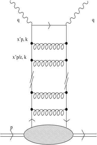
Figure 1: Ladder diagram generating double logarithmic terms in the non-singlet spin structure function $g_{1}^{NS}$.

Figure 2: Ladder elements for a singlet case

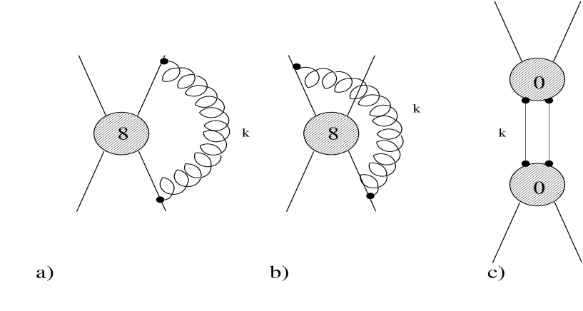
Figure 3: Non-ladder contributions containing a), b) soft gluon or c) soft quark attached to the quark-quark scattering amplitude

The sum of double logarithmic $ln^{2}(1/x)$ terms corresponding to ladder diagrams is generated by the following integral equations (see Figs.1, 2) :

$$f_{j}(x^{\prime},k^{2})=f^{(0)}_{j}(x^{\prime},k^{2})+{\alpha_{s}\over 2\pi}\Delta P_{qq}(0)\int_{x^{\prime}}^{1}{dz\over z}\int_{k_{0}^{2}}^{k^{2}/z}{dk^{\prime 2}\over k^{\prime 2}}f_{j}\left({x^{\prime}\over z},k^{\prime 2}\right),$$ (17)

where $j=u_{v},d_{v},us$, and :

$$f_{\Sigma}(x^{\prime},k^{2})=f^{(0)}_{\Sigma}(x^{\prime},k^{2})+{\alpha_{s}\over 2\pi}\int_{x^{\prime}}^{1}{dz\over z}\int_{k_{0}^{2}}^{k^{2}/z}{dk^{\prime 2}\over k^{\prime 2}}\left[\Delta P_{qq}(0)f_{\Sigma}\left({x^{\prime}\over z},k^{\prime 2}\right)+\Delta P_{qg}(0)f_{g}\left({x^{\prime}\over z},k^{\prime 2}\right)\right],$$

$$f_{g}(x^{\prime},k^{2})=f^{(0)}_{g}(x^{\prime},k^{2})+{\alpha_{s}\over 2\pi}\int_{x^{\prime}}^{1}{dz\over z}\int_{k_{0}^{2}}^{k^{2}/z}{dk^{\prime 2}\over k^{\prime 2}}\left[\Delta P_{gq}(0)f_{\Sigma}\left({x^{\prime}\over z},k^{\prime 2}\right)+\Delta P_{gg}(0)f_{g}\left({x^{\prime}\over z},k^{\prime 2}\right)\right]$$

(18)

with $\Delta P_{ij}(0)\equiv\Delta P_{ij}(z=0)$ given by Eq. (9).

The variables $k^{2}$($k^{\prime 2}$) denote the transverse momenta squared of the quarks (gluons) exchanged along the ladder, $k_{0}^{2}$ is the infrared cut-off and the inhomogeneous terms $f_{i}^{(0)}(x^{\prime},k^{2})$ will be specified later. The integration limit $k^{2}/z$ follows from the requirement that the virtuality of the quarks (gluons) exchanged along the ladder is controlled by the tranverse momentum squared.

Equation (17) is similar to the corresponding equation in QED describing the double logarithmic resummation generated by ladder diagrams with fermion exchange [16]. The problem of double logarithimc asymptotics in QCD in the non-singlet channels was also discussed in Ref. [17, 18, 19].

Equations (17, 18) generate singular power behaviour of the spin dependent parton distributions and of the spin dependent structure functions $g_{1}$ at small $x$ i.e.

$$g_{1}^{NS}(x,Q^{2})\sim x^{-\lambda_{NS}},$$

$$g_{1}^{S}(x,Q^{2})\sim x^{-\lambda_{S}},$$

$$\Delta G(x,Q^{2})\sim x^{-\lambda_{S}},$$ (19)

where $g_{1}^{NS}=g_{1}^{p}-g_{1}^{n}$ and $g_{1}^{S}=g_{1}^{p}+g_{1}^{n}$ respectively, and $\Delta G$ is the spin dependent gluon distribution. The behaviour of spin structure functions reflects the small $x^{\prime}$ behaviour of their unintegrated distributions. Exponents $\lambda_{NS,S}$ are given by the following formulas:

$$\lambda_{NS}=2\sqrt{\left[{\alpha_{s}\over 2\pi}\Delta P_{qq}(0)\right]},$$ (20)

$$\lambda_{S}=2\sqrt{\left[{\alpha_{s}\over 2\pi}\lambda_{0}^{+}\right]},$$ (21)

where $\lambda_{0}^{+}$ is given by Eq. (4). The power-like behaviour (19) with the exponents $\lambda_{NS,S}$ given by Eq. (21) remains the leading small $x$ behaviour of the structure functions provided that their non-perturbative parts are less singular. This takes place if the latter are assumed to have the Regge pole like behaviour with the corresponding intercept(s) being near $0$.

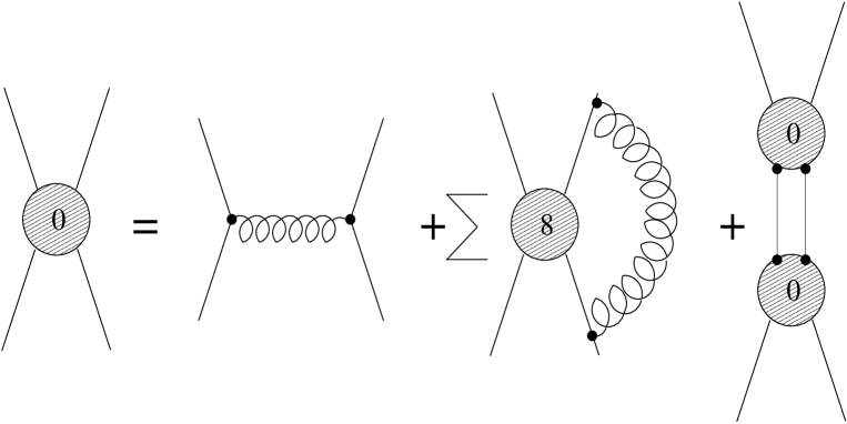
Figure 4: Infrared evolution equation for partial wave matrix $F_{0}$

The exponents $\lambda_{NS}$ and $\lambda_{S}$ correspond to the leading singularities of the moment functions $\bar{f}_{i}(\omega,k^{2})$ ( $\Delta\bar{p}_{i}(\omega,Q^{2})$ ) for $i={\small NS}(i=u_{v},d_{v},us)$ and $i=\Sigma,i=g$ respectively in the $\omega$ plane. The moment functions $\bar{f}_{i}(\omega,k^{2})$ and $\Delta\bar{p}_{i}(\omega,Q^{2})$ are defined in a conventional way :

$$\bar{f}_{i}(\omega,k^{2})=\int_{0}^{1}dx^{\prime}x^{\prime\omega-1}f_{i}(x^{\prime},k^{2}),$$

$$\Delta\bar{p}_{i}(\omega,Q^{2})=\int_{0}^{1}dxx^{\omega-1}\Delta p_{i}(x,Q^{2}).$$ (22)

Ladder equations (17), (18) in $\omega-$space take then the form :

$$\bar{f}_{i}(\omega,k^{2}) = \bar{f}_{i}^{(0)}(\omega,k^{2})+{\bar{\alpha}_{s}\over\omega}\Delta P_{qq}(0)\left[\int_{k_{0}^{2}}^{k^{2}}{dk^{\prime 2}\over k^{\prime 2}}\bar{f}_{i}(\omega,k^{\prime 2})+\int_{k^{2}}^{\infty}{dk^{\prime 2}\over k^{\prime 2}}\left({k^{2}\over k^{\prime 2}}\right)^{\omega}\bar{f}_{i}(\omega,k^{\prime 2})\right],$$ (23)

$${\bf\bar{f}}_{S}(\omega,k^{2}) = {\bf\bar{f}}_{S}^{(0)}(\omega,k^{2})+{\bar{\alpha}_{s}\over\omega}{\bf M}_{0}\left[\int_{k_{0}^{2}}^{k^{2}}{dk^{\prime 2}\over k^{\prime 2}}{\bf\bar{f}}_{S}(\omega,k^{\prime 2})+\int_{k^{2}}^{\infty}{dk^{\prime 2}\over k^{\prime 2}}\left({k^{2}\over k^{\prime 2}}\right)^{\omega}{\bf\bar{f}}_{S}(\omega,k^{\prime 2})\right],$$ (24)

where $i=u_{v},d_{v},us$, and $\bar{\alpha}_{s}$ is defined as :

$$\bar{\alpha}_{s}=\frac{\alpha_{s}}{2\pi},$$ (25)

and :

$${\bf\bar{f}}_{S}(\omega,k^{2}) = \left(\begin{array}[]{cc}\bar{f}_{\Sigma}(\omega,k^{2})\\ \bar{f}_{g}(\omega,k^{2})\\ \end{array}\right),$$ (28)

$${\bf M}_{0}\equiv{\bf\Delta P}(0) = \left(\begin{array}[]{cc}\Delta P_{qq}(0)&\Delta P_{qg}(0)\\ \Delta P_{gq}(0)&\Delta P_{gg}(0)\\ \end{array}\right).$$ (31)

The inhomogeneous terms $\bar{f}_{i}^{(0)}$ and ${\bf\bar{f}}_{S}^{(0)}$ are related to the moment functions $\Delta\bar{p}_{i}^{(0)}(\omega)$ of the nonperturbative parts $\Delta p_{i}^{(0)}(x)$ and ${\bf\Delta p}_{S}^{(0)}(x)$ of the integrated distributions in the following way :

$$\bar{f}_{i}^{(0)}(\omega,k^{2}) = \bar{\alpha}_{s}{\Delta P_{qq}(0)\over\omega}\Delta\bar{p}_{i}^{(0)}(\omega),$$

$${\bf\bar{f}}_{S}^{(0)}(\omega,k^{2}) = \bar{\alpha}_{s}{{\bf M_{0}}\over\omega}{\bf\Delta\bar{p}}_{S}^{(0)}(\omega).$$ (32)

For fixed coupling $\alpha_{s}$ one may obtain analytic solution of (23), (24) :

$$\bar{f}_{i}(\omega,k^{2})=R_{i}(\bar{\alpha}_{s},\omega)\left({k^{2}\over k_{0}^{2}}\right)^{\gamma_{NS}(\alpha_{s},\omega)},$$ (33)

$${\bf\bar{f}}_{S}(\omega,k^{2})=\left({k^{2}\over k_{0}^{2}}\right)^{\mbox{\boldmath$\gamma$}_{S}(\alpha_{s},\omega)}{\bf R}_{S}(\bar{\alpha}_{s},\omega),$$ (34)

where $\gamma_{NS}$, ${\mbox{\boldmath$\gamma$}_{S}}$ represent anomalous dimensions for the non-singlet and singlet case respectively, and are equal to :

$$\gamma_{NS}(\omega,\alpha_{s}) = {\omega-\sqrt{\omega^{2}-4\Delta P_{qq}(0)\bar{\alpha}_{s}}\over 2}$$ (35)

$${\mbox{\boldmath$\gamma$}}_{S}(\omega,\alpha_{s}) = {\omega-\sqrt{\omega^{2}-4{\bf M_{0}}\bar{\alpha}_{s}}\over 2},$$ (36)

and $R_{i}(\bar{\alpha}_{s},\omega)$ and ${\bf R}_{S}(\bar{\alpha}_{s},\omega)$ are given by the following equations :

$$R_{i}(\bar{\alpha}_{s},\omega)=\gamma_{NS}(\bar{\alpha}_{s},\omega)\Delta\bar{p}_{i}^{(0)}(\omega)$$

$${\bf R}_{S}(\bar{\alpha}_{s},\omega)={\mbox{\boldmath$\gamma$}_{S}}(\bar{\alpha}_{s},\omega){\bf\Delta\bar{p}}_{S}^{(0)}(\omega).$$ (37)

It should be reminded that for the singlet case only the eigenvalues of $\mbox{\boldmath$\gamma$}_{S}$ contribute to the final solution. The solution takes then the explicit form :

$$\bar{f}_{\Sigma,g}(\omega,k^{2})=R_{\Sigma,g}^{+}(\omega,\alpha_{s},)\left({k^{2}\over k_{0}^{2}}\right)^{\gamma^{+}(\omega,\alpha_{s})}+R_{\Sigma,g}^{-}(\omega,\alpha_{s})\left({k^{2}\over k_{0}^{2}}\right)^{\gamma^{-}(\omega,\alpha_{s})},$$ (38)

where $\lambda_{0}^{+}$, $\lambda_{0}^{-}$ denote eigenvalues of of $\mbox{\boldmath$\gamma$}_{S}$ :

$$\gamma^{\pm}(\omega,\alpha_{s})={{\omega-\sqrt{\omega^{2}-4{\bar{\alpha}_{s}}\lambda^{\pm}_{0}}}\over 2},$$ (39)

and $\lambda^{+}_{0}$ (the eigenvalue of ${\bf M}_{0}$) is defined by equation (4) while $\lambda^{-}_{0}$ reads:

$$\lambda^{-}_{0}={\Delta P_{qq}(0)+\Delta P_{gg}(0)-\sqrt{(\Delta P_{qq}(0)-\Delta P_{gg}(0))^{2}+4\Delta P_{qg}(0)\Delta P_{gq}(0)}\over 2}.$$ (40)

It can be shown that the moment functions $\Delta\bar{p}_{i}(\omega,Q^{2})$ and ${\bf\Delta\bar{p}}_{S}(\omega,Q^{2})$ of the spin dependent distributions have the familiar RG form (for the fixed coupling) :

$$\Delta\bar{p}_{i}(\omega,Q^{2})=\bar{R}_{i}(\bar{\alpha}_{s},\omega)\left({Q^{2}\over k_{0}^{2}}\right)^{\gamma_{NS}(\bar{\alpha}_{s},\omega)}+O(k_{0}^{2}/Q^{2})$$

$${\bf\Delta\bar{p}}_{S}(\omega,Q^{2})=\left({Q^{2}\over k_{0}^{2}}\right)^{{\mbox{\boldmath$\gamma$}_{S}}(\bar{\alpha}_{s},\omega)}{\bf\bar{R}}_{S}(\bar{\alpha}_{s},\omega)+O(k_{0}^{2}/Q^{2}),$$ (41)

where

$$\bar{R}_{i}(\bar{\alpha}_{s},\omega)={\Gamma(\gamma_{NS}(\bar{\alpha}_{s},\omega)+1)\Gamma(\omega-\gamma_{NS}(\bar{\alpha}_{s},\omega))\over\Gamma(\omega)}\Delta\bar{p}_{i}^{(0)}(\omega)$$

$${\bf\bar{R}}_{S}(\bar{\alpha}_{s},\omega)={\Gamma({\mbox{\boldmath$\gamma$}_{S}}(\bar{\alpha}_{s},\omega)+1)\Gamma(\omega-{\mbox{\boldmath$\gamma$}_{S}}(\bar{\alpha}_{s},\omega))\over\Gamma(\omega)}{\bf\Delta\bar{p}}_{S}^{(0)}(\omega).$$ (42)

To derive (41) we notice that equation (12) implies the following relation between the moment functions $\Delta\bar{p}_{i}(\omega,Q^{2})$ and $\bar{f}_{i}(\omega,k^{2})$:

$$\Delta\bar{p}_{i}(\omega,Q^{2})=\Delta\bar{p}_{i}^{(0)}(\omega)+\int_{k_{0}^{2}}^{\infty}{dk^{2}\over k^{2}}\left(1+{k^{2}\over Q^{2}}\right)^{-\omega}\bar{f}_{i}(\omega,k^{2}).$$ (43)

Substituting expressions (33) and (34) into (43) and taking into account equation (37) we obtain equation (41).

Equations (35), (36) imply that the anomalous dimensions $\gamma_{NS}(\omega,\alpha_{s})$ and $\gamma^{\pm}(\omega,\alpha_{s})$ have the branch point singularities in $\omega$ plane located at $\omega=2\sqrt{\bar{\alpha}_{s}\Delta P_{qq}(0)}$ and at $\omega=2\sqrt{\bar{\alpha}_{s}\lambda_{0}^{\pm}}$ respectively. The small $x$ behaviour of the parton distributions and of the structure functions which is given by equations (19) with the exponents $\lambda_{NS}$ and $\lambda_{S}$ defined by equations (20) and (21) just reflects the fact that this behaviour is controlled by the leading singularities in the $\omega$ plane.

It may be seen from equations (41,42) that the branch point singularities of anomalous dimensions are also present in the prefactors $\bar{R}_{i}(\bar{\alpha}_{s},\omega)$ and ${\bf\bar{R}}_{S}(\bar{\alpha}_{s},\omega)$ and so the low $x$ behaviour of spin dependent structure functions given by equations (19) is expected to hold for arbitrary values of the scale $Q^{2}$.

Complete sum of double logarithmic $ln^{2}(1/x)$ terms does also include the non-ladder bremsstrahlung contributions besides the ladder ones. Expressions (20), (21) corresponding to the ladder diagrams are therefore only approximate. The method of implementing the non-ladder bremsstrahlung corrections into the double logarithmic resummation was originally proposed by Kirschner, Lipatov [17], and applied for the case of DIS small $x$ asymptotics in [8, 9], [11]. Below we show how to implement these terms within our formalism. In order to include the non-ladder corrections to the double logarithmic asymptotics we use the infrared evolution equations derived in [8, 9, 17]. The evolution equations for singlet partial waves $F_{0}$, $F_{8}$ (see Fig. 4 ) :

$${\bf F}_{0,8}=\left(\begin{array}[]{cc}F_{qq}^{(0,8)}&F_{qg}^{(0,8)}\\ F_{gq}^{(0,8)}&F_{gg}^{(0,8)}\\ \end{array}\right)$$ (44)

have the form :

$${\bf F}_{0}(\omega,\alpha_{s}) = \frac{8\pi^{2}\bar{\alpha}_{s}}{\omega}{\bf M}_{0}-\frac{4\bar{\alpha}_{s}}{\omega^{2}}{\bf F}_{8}(\omega,\alpha_{s}){\bf G}_{0}+\frac{1}{8\pi^{2}\omega}{\bf F}_{0}^{2}(\omega,\alpha_{s})$$ (45)

$${\bf F}_{8}(\omega,\alpha_{s}) = \frac{8\pi^{2}\bar{\alpha}_{s}}{\omega}{\bf M}_{8}+\frac{\bar{\alpha}_{s}N}{\omega}\frac{d}{d\omega}{\bf F}_{8}(\omega,\alpha_{s})+\frac{1}{8\pi^{2}\omega}{\bf F}_{8}^{2}(\omega,\alpha_{s}),$$ (46)

where ${\bf M}_{0}$ (cf. 31), ${\bf M}_{8}$ are splitting functions matrices in colour singlet and octet $t-$channel, and ${\bf G}_{0}$ contains colour factors resulting from attaching the soft gluon to external legs of the scattering amplitude :

$${\bf M}_{8} = \left(\begin{array}[]{cc}-{1\over 2N}&-{N_{F}\over 2}\\ N&2N\\ \end{array}\right),$$ (49)

$${\bf G}_{0} = \left(\begin{array}[]{cc}{N^{2}-1\over 2N}&0\\ 0&N\\ \end{array}\right).$$ (52)

Non-singlet contribution comes from $F_{0}^{qq}$ partial wave, as expected. Only the partial waves ${\bf F}_{0}$ are contributing to the anomalous dimensions. An explicit relation between partial waves and anomalous dimension reads :

$${\bf F}_{0} = 8\pi^{2}{\mbox{\boldmath$\gamma$}}_{S}^{RES}$$ (53)

$$F_{qq}^{(0)} = 8\pi^{2}\gamma_{NS}^{RES}$$ (54)

and it depends already on resummed anomalous dimensions $\gamma^{RES}$ with all infrared non-ladder corrections included. Equation (45) for ${\bf F}_{0}$ may be solved analytically generating the following expressions for anomalous dimensions :

$$\gamma_{NS}^{RES}(\alpha_{s},\omega) = \frac{\omega}{2}\Biggl{(}1-\sqrt{1-\frac{4\bar{\alpha}_{s}}{\omega}\Biggl{(}\frac{\Delta P_{qq}(0)}{\omega}-\frac{({\bf F}_{8}(\omega){\bf G}_{0})_{qq}}{2\pi^{2}\omega^{2}}\Biggr{)}}\Biggr{)}$$ (55)

$${\mbox{\boldmath$\gamma$}}_{S}^{RES}(\alpha_{s},\omega) = \frac{\omega}{2}\Biggl{(}1-\sqrt{1-\frac{4\bar{\alpha}_{s}}{\omega}\Biggl{(}\frac{{\bf M}_{0}}{\omega}-\frac{{\bf F}_{8}(\omega){\bf G}_{0}}{2\pi^{2}\omega^{2}}\Biggr{)}}\Biggr{)}.$$ (56)

Comparing the expressions for anomalous dimensions with and without the non-ladder contribution (35), (36), (55), (56) one may notice that the bremsstrahlung contribution adds an additional term under the square root of $\gamma$’s :

$$\sqrt{1-\frac{4\bar{\alpha}_{s}}{\omega}\frac{{\bf M}_{0}}{\omega}}\,\,\,\,\,{\bf\longrightarrow}\,\,\,\,\,\sqrt{1-\frac{4\bar{\alpha}_{s}}{\omega}\Biggl{(}\frac{{\bf M}_{0}}{\omega}-\frac{{\bf F}_{8}(\omega){\bf G}_{0}}{2\pi^{2}\omega^{2}}\Biggr{)}}.$$ (57)

The same anomalous dimensions would be obtained if we modified the kernels of equations (23) and (24) by setting $\bar{\alpha}_{s}\left({{\bf M_{0}}\over\omega}-{{\bf F_{8}}(\omega){\bf G_{0}}\over 2\pi^{2}\omega^{2}}\right)$ in place of $\bar{\alpha}_{s}{{\bf M_{0}}\over\omega}$. The modified equations then read:

$$\bar{f}_{i}(\omega,k^{2}) = \bar{f}_{i}^{(0)}(\omega,k^{2})$$ (58)

$$+ \bar{\alpha}_{s}\left({{\Delta P(0)}\over\omega}-{{\bf F_{8}}(\omega){\bf G_{0}}\over 2\pi^{2}\omega^{2}}\right)_{qq}\left[\int_{k_{0}^{2}}^{k^{2}}{dk^{\prime 2}\over k^{\prime 2}}\bar{f}_{i}(\omega,k^{\prime 2})+\int_{k^{2}}^{\infty}{dk^{\prime 2}\over k^{\prime 2}}\left({k^{2}\over k^{\prime 2}}\right)^{\omega}\bar{f}_{i}(\omega,k^{\prime 2})\right],$$

$${\bf\bar{f}}_{S}(\omega,k^{2}) = {\bf\bar{f}}_{S}^{(0)}(\omega,k^{2})$$ (59)

$$+ \bar{\alpha}_{s}\left({{\bf M_{0}}\over\omega}-{{\bf F_{8}}(\omega){\bf G_{0}}\over 2\pi^{2}\omega^{2}}\right)\left[\int_{k_{0}^{2}}^{k^{2}}{dk^{\prime 2}\over k^{\prime 2}}{\bf\bar{f}}_{S}(\omega,k^{\prime 2})+\int_{k^{2}}^{\infty}{dk^{\prime 2}\over k^{\prime 2}}\left({k^{2}\over k^{\prime 2}}\right)^{\omega}{\bf\bar{f}}_{S}(\omega,k^{\prime 2})\right],$$

The corresponding equations for the functions $f_{i}(x^{\prime},k^{2})$ and for for ${\bf f}_{S}$ have the form :

$$f_{j}(x^{\prime},k^{2})=f^{(0)}_{j}(x^{\prime},k^{2}) + {\bar{\alpha}_{s}}\,\Delta P_{qq}(0)\int_{x^{\prime}}^{1}{dz\over z}\int_{k_{0}^{2}}^{k^{2}/z}{dk^{\prime 2}\over k^{\prime 2}}f_{j}\left({x^{\prime}\over z},k^{\prime 2}\right)$$ (60)

$$- {\bar{\alpha}_{s}}\int_{x^{\prime}}^{1}{dz\over z}\Biggl{(}\Biggl{[}\frac{\tilde{\bf F}_{8}}{\omega^{2}}\Biggr{]}(z)\frac{{\bf G}_{0}}{2\pi^{2}}\Biggr{)}_{qq}\int_{k_{0}^{2}}^{k^{2}}{dk^{\prime 2}\over k^{\prime 2}}f_{j}\left({x^{\prime}\over z},k^{\prime 2}\right)$$

$$- {\bar{\alpha}_{s}}\int_{x^{\prime}}^{1}{dz\over z}\int_{k^{2}}^{k^{2}/z}{dk^{\prime 2}\over k^{\prime 2}}\Biggl{(}\Biggl{[}\frac{\tilde{\bf F}_{8}}{\omega^{2}}\Biggr{]}\Biggl{(}\frac{k^{\prime 2}}{k^{2}}z\Biggr{)}\frac{{\bf G}_{0}}{2\pi^{2}}\Biggr{)}_{qq}f_{j}\left({x^{\prime}\over z},k^{\prime 2}\right),$$

where $j=u_{v},d_{v},us$, and :

$${\bf f}_{S}(x^{\prime},k^{2})={\bf f}^{(0)}_{S}(x^{\prime},k^{2}) + {\bar{\alpha}_{s}}\,{\bf M}_{0}\int_{x^{\prime}}^{1}{dz\over z}\int_{k_{0}^{2}}^{k^{2}/z}{dk^{\prime 2}\over k^{\prime 2}}{\bf f}_{S}\left({x^{\prime}\over z},k^{\prime 2}\right)$$ (61)

$$- {\bar{\alpha}_{s}}\int_{x^{\prime}}^{1}{dz\over z}\Biggl{[}\frac{\tilde{\bf F}_{8}}{\omega^{2}}\Biggr{]}(z)\frac{{\bf G}_{0}}{2\pi^{2}}\int_{k_{0}^{2}}^{k^{2}}{dk^{\prime 2}\over k^{\prime 2}}{\bf f}_{S}\left({x^{\prime}\over z},k^{\prime 2}\right)$$

$$- {\bar{\alpha}_{s}}\int_{x^{\prime}}^{1}{dz\over z}\int_{k^{2}}^{k^{2}/z}{dk^{\prime 2}\over k^{\prime 2}}\Biggl{[}\tilde{\frac{{\bf F}_{8}}{\omega^{2}}}\Biggr{]}\Biggl{(}\frac{k^{\prime 2}}{k^{2}}z\Biggr{)}\frac{{\bf G}_{0}}{2\pi^{2}}{\bf f}_{S}\left({x^{\prime}\over z},k^{\prime 2}\right),$$

where $\Biggl{[}\frac{\tilde{\bf F}_{8}}{\omega^{2}}\Biggr{]}(z)$ denotes the inverse Mellin transform of $\frac{{\bf F}_{8}}{\omega^{2}}$ :

$$\Biggl{[}\frac{\tilde{\bf F}_{8}}{\omega^{2}}\Biggr{]}(z)=\int_{\delta-i\infty}^{\delta+i\infty}{d\omega\over 2\pi i}z^{-\omega}\frac{{\bf F}_{8}(\omega)}{\omega^{2}}.$$ (62)

with the integration contour located to the right of the singularities of the function $\frac{{\bf F}_{8}(\omega)}{\omega^{2}}$.

To obtain $F_{8}$ we have to solve Eq. (46). The exact solution presented in [8, 9] may be expressed in terms of parabolic cylinder functions :

$$f_{8}^{\pm}=8\pi^{2}\bar{\alpha}_{s}{d\over d\omega}ln(e^{z^{2}/4}D_{p\pm}(z)),$$ (63)

where $f_{8}^{\pm}$ are two eigenvalues of matrix ${\bf F}_{8}(\omega)$ determined in a basis of eigenvectors of ${\bf M}_{8}$, and :

$$z={\omega\over\omega_{0}},\,\,\omega_{0}=\sqrt{N\bar{\alpha}_{s}},\,\,p_{\pm}={\lambda_{8}^{\pm}\over N},$$ (64)

where $\lambda_{8}^{\pm}$ denote eigenvalues of matrix ${\bf M}_{8}$.

For a general solution (63) the inverse Mellin transform of $\frac{{\bf F}_{8}(\omega)}{\omega^{2}}$ does not exist in the analytic form. However, it was checked in [8] that approximate form of $F_{8}(\omega)$ determined in the large $N$ limit is a good approximation for fixed $\alpha_{s}$. The large $N$ expansion proposed in [8] reduces $F_{8}$ to the Born term. In our case it implies :

$${\bf F}_{8}^{Born}(\omega)\approx 8\pi^{2}\bar{\alpha}_{s}\frac{{\bf M}_{8}}{\omega}.$$ (65)

The inverse Melin transform then reads :

$$\Biggl{[}\frac{\tilde{\bf F}_{8}^{Born}}{\omega^{2}}\Biggr{]}(z)=4\pi^{2}\bar{\alpha}_{s}{\bf M}_{8}ln^{2}(z).$$ (66)

The different large $N$ approach which we propose here uses the approximate form of ${\bf M}_{0}$, ${\bf M}_{8}$, ${\bf G}_{0}$ (31), (52) :

$${\bf M}_{0}\approx\left(\begin{array}[]{cc}N/2&0\\ N&4N\\ \end{array}\right),\,\,{\bf M}_{8}\approx\left(\begin{array}[]{cc}0&0\\ N&2N\\ \end{array}\right),\,\,{\bf G}_{0}\approx\left(\begin{array}[]{cc}N/2&0\\ 0&N\\ \end{array}\right),\,\,$$ (67)

where we have neglected all terms of the order less than $O(N)$. Then the two components of $F_{8}$ simplify :

$$f_{8}^{+,large\,N}(\omega) = 16\pi^{2}\frac{\omega\omega_{0}^{2}}{\omega^{2}-\omega_{0}^{2}},$$

$$f_{8}^{-,large\,N}(\omega) = 0,$$ (68)

and the inverse Mellin transform of $\frac{f_{8}^{+,large\,N}}{\omega^{2}}$ reads :

$$\Biggl{[}\frac{\tilde{f}_{8}^{+,large\,N}}{\omega^{2}}\Biggr{]}(z)=8\pi^{2}(z^{\omega_{0}}+z^{-\omega_{0}}-2).$$ (69)

We have checked that both approaches give similar evolution of polarized structure function $g_{1}$ and gluon distribution. Moreover, the branch point singularities dominating the small $x$ behaviour of $g^{NS}_{1}$ and $g^{S}_{1}$ behave also in similar way. For the non-singlet case the leading singularity may be determined from the Eq. (55) as :

$$1-\frac{4\bar{\alpha}_{s}}{\omega}\Biggl{(}\frac{\Delta P_{qq}(0)}{\omega}-\frac{({\bf F}_{8}(\omega){\bf G}_{0})_{qq}}{2\pi^{2}\omega^{2}}\Biggr{)}=0$$ (70)

and for the ladder case it reads (cf. (20)) :

$$\lambda^{NS}=2\sqrt{\frac{N^{2}-1}{2N}\bar{\alpha}_{s}}\approx 0.39,$$ (71)

where it was assumed that $\alpha_{s}=0.18$, $N=3$, $N_{F}=3$. Including the non-ladder resummation gives :

$$\lambda^{NS,Born} \approx 2\sqrt{\frac{N^{2}-1}{2N}\bar{\alpha}_{s}}\Biggl{(}1+\frac{1}{2N^{2}}\Biggr{)}\approx 0.41,$$

$$\lambda^{NS,large\,N} \approx 2\sqrt{\frac{N}{2}\bar{\alpha}_{s}}\approx 0.42.$$ (72)

The singlet dominating singularity fulfills the relation (cf. (56)) :

$$det\Biggl{(}1-\frac{4\bar{\alpha}_{s}}{\omega}\Biggl{(}\frac{{\bf M}_{0}}{\omega}-\frac{{\bf F}_{8}(\omega){\bf G}_{0}}{2\pi^{2}\omega^{2}}\Biggr{)}\Biggr{)}=0$$ (73)

and for the ladder case it may be easily determined as :

$$\lambda^{S}=2\sqrt{\lambda^{+}_{0}\bar{\alpha}_{s}}\approx 1.13$$ (74)

($\alpha_{s}=0.18$, $N=3$, $N_{F}=3$). The non-ladder resummation changes the singularity point into :

$$\lambda^{S,Born} \approx 1.01$$

$$\lambda^{S,large\,N} \approx 1.07.$$ (75)

One may notice that for both singlet and non-singlet case the influence of the non-ladder resummation on the singularities is of the order 10%. Since the differences between Born and large N approaches are very small, in the following discussion we restrict to the Born approximation for ${\bf F}_{8}$.

4 Unified evolution equation

In order to make the quantitative predictions one has to constrain the structure functions by the existing data at large and moderately small values of $x$. For such values of $x$ however the equations (60) and (61) are inaccurate. In this region one should use the conventional Altarelli-Parisi equations with complete splitting functions $\Delta P_{ij}(z)$ and not restrict oneself to the effect generated only by their $z\rightarrow 0$ part. Following refs. [13, 15] we do therefore extend equations (60,61) and add to their right hand side the contributions coming from the remaining parts of the splitting functions $\Delta P_{ij}(z)$. We also allow the coupling $\alpha_{s}$ to run setting $k^{2}$ as the relevant scale. In this way we obtain unified system of equations which contain both the complete LO Altarelli-Parisi evolution and the double logarithmic $ln^{2}(1/x)$ effects at low $x$. The corresponding system of equations reads :

$$f_{k}(x^{\prime},k^{2})=f^{(0)}_{k}(x^{\prime},k^{2}) + {\alpha_{s}(k^{2})\over 2\pi}{4\over 3}\int_{x^{\prime}}^{1}{dz\over z}\int_{k_{0}^{2}}^{k^{2}/z}{dk^{\prime 2}\over k^{\prime 2}}f_{k}\left({x^{\prime}\over z},k^{\prime 2}\right)$$

$$\hskip 38.74985pt{\bf(\hskip 11.62495ptLadder\hskip 11.62495pt)}$$

$$+ {\alpha_{s}(k^{2})\over 2\pi}\int_{k_{0}^{2}}^{k^{2}}{dk^{\prime 2}\over k^{\prime 2}}{4\over 3}\int_{x^{\prime}}^{1}{dz\over z}{(z+z^{2})f_{k}({x^{\prime}\over z},k^{\prime 2})-2zf_{k}(x^{\prime},k^{\prime 2})\over 1-z}$$

$$+ {\alpha_{s}(k^{2})\over 2\pi}\int_{k_{0}^{2}}^{k^{2}}{dk^{\prime 2}\over k^{\prime 2}}\left[2+{8\over 3}ln(1-x^{\prime})\right]f_{k}(x^{\prime},k^{\prime 2})$$

$$\hskip 38.74985pt{\bf(\hskip 11.62495ptA-P\hskip 15.49994pt)}$$

$$- {\alpha_{s}(k^{2})\over 2\pi}\int_{x^{\prime}}^{1}{dz\over z}\Biggl{(}\Biggl{[}\frac{\tilde{\bf F}_{8}}{\omega^{2}}\Biggr{]}(z)\frac{{\bf G}_{0}}{2\pi^{2}}\Biggr{)}_{qq}\int_{k_{0}^{2}}^{k^{2}}{dk^{\prime 2}\over k^{\prime 2}}f_{j}\left({x^{\prime}\over z},k^{\prime 2}\right)$$

$$- {\alpha_{s}(k^{2})\over 2\pi}\int_{x^{\prime}}^{1}{dz\over z}\int_{k^{2}}^{k^{2}/z}{dk^{\prime 2}\over k^{\prime 2}}\Biggl{(}\Biggl{[}\frac{\tilde{\bf F}_{8}}{\omega^{2}}\Biggr{]}\Biggl{(}\frac{k^{\prime 2}}{k^{2}}z\Biggr{)}\frac{{\bf G}_{0}}{2\pi^{2}}\Biggr{)}_{qq}f_{j}\left({x^{\prime}\over z},k^{\prime 2}\right),$$

$$\hskip 38.74985pt{\bf(Non-ladder)}$$

where $k=u_{v},d_{v},us$,

$$f_{\Sigma}(x^{\prime},k^{2})=f^{(0)}_{\Sigma}(x^{\prime},k^{2}) + {\alpha_{s}(k^{2})\over 2\pi}\int_{x^{\prime}}^{1}{dz\over z}\int_{k_{0}^{2}}^{k^{2}/z}{dk^{\prime 2}\over k^{\prime 2}}{4\over 3}f_{\Sigma}\left({x^{\prime}\over z},k^{\prime 2}\right)$$

$$- {\alpha_{s}(k^{2})\over 2\pi}\int_{x^{\prime}}^{1}{dz\over z}\int_{k_{0}^{2}}^{k^{2}/z}N_{F}{dk^{\prime 2}\over k^{\prime 2}}f_{g}\left({x^{\prime}\over z},k^{\prime 2}\right)$$

$$\hskip 38.74985pt{\bf(\hskip 11.62495ptLadder\hskip 11.62495pt)}$$

$$+ {\alpha_{s}(k^{2})\over 2\pi}\int_{k_{0}^{2}}^{k^{2}}{dk^{\prime 2}\over k^{\prime 2}}{4\over 3}\int_{x^{\prime}}^{1}{dz\over z}{(z+z^{2})f_{\Sigma}({x^{\prime}\over z},k^{\prime 2})-2zf_{\Sigma}(x^{\prime},k^{\prime 2})\over 1-z}$$

$$+ {\alpha_{s}(k^{2})\over 2\pi}\int_{k_{0}^{2}}^{k^{2}}{dk^{\prime 2}\over k^{\prime 2}}\left[2+{8\over 3}ln(1-x^{\prime})\right]f_{\Sigma}(x^{\prime},k^{\prime 2})$$

$$+ {\alpha_{s}(k^{2})\over 2\pi}\int_{k_{0}^{2}}^{k^{2}}{dk^{\prime 2}\over k^{\prime 2}}\int_{x^{\prime}}^{1}{dz\over z}2zN_{F}f_{g}({x^{\prime}\over z},k^{\prime 2})$$

$$\hskip 38.74985pt{\bf(\hskip 11.62495ptA-P\hskip 15.49994pt)}$$

$$- {\alpha_{s}(k^{2})\over 2\pi}\int_{x^{\prime}}^{1}{dz\over z}\Biggl{(}\Biggl{[}\frac{\tilde{\bf F}_{8}}{\omega^{2}}\Biggr{]}(z)\frac{{\bf G}_{0}}{2\pi^{2}}\Biggr{)}_{qq}\int_{k_{0}^{2}}^{k^{2}}{dk^{\prime 2}\over k^{\prime 2}}f_{\Sigma}\left({x^{\prime}\over z},k^{\prime 2}\right)$$

$$- {\alpha_{s}(k^{2})\over 2\pi}\int_{x^{\prime}}^{1}{dz\over z}\int_{k^{2}}^{k^{2}/z}{dk^{\prime 2}\over k^{\prime 2}}\Biggl{(}\Biggl{[}\frac{\tilde{\bf F}_{8}}{\omega^{2}}\Biggr{]}\Biggl{(}\frac{k^{\prime 2}}{k^{2}}z\Biggr{)}\frac{{\bf G}_{0}}{2\pi^{2}}\Biggr{)}_{qg}f_{g}\left({x^{\prime}\over z},k^{\prime 2}\right),$$

$$\hskip 38.74985pt{\bf(Non-ladder)}$$

$$f_{g}(x^{\prime},k^{2})=f^{(0)}_{g}(x^{\prime},k^{2}) + {\alpha_{s}(k^{2})\over 2\pi}\int_{x^{\prime}}^{1}{dz\over z}\int_{k_{0}^{2}}^{k^{2}/z}{dk^{\prime 2}\over k^{\prime 2}}{8\over 3}f_{\Sigma}\left({x^{\prime}\over z},k^{\prime 2}\right)$$

$$+ {\alpha_{s}(k^{2})\over 2\pi}\int_{x^{\prime}}^{1}{dz\over z}\int_{k_{0}^{2}}^{k^{2}/z}{dk^{\prime 2}\over k^{\prime 2}}12f_{g}\left({x^{\prime}\over z},k^{\prime 2}\right)$$

$$\hskip 38.74985pt{\bf(\hskip 11.62495ptLadder\hskip 11.62495pt)}$$

$$+ {\alpha_{s}(k^{2})\over 2\pi}\int_{k_{0}^{2}}^{k^{2}}{dk^{\prime 2}\over k^{\prime 2}}\int_{x^{\prime}}^{1}{dz\over z}(-{4\over 3})zf_{\Sigma}\left({x^{\prime}\over z},k^{\prime 2}\right)$$

$$+ {\alpha_{s}(k^{2})\over 2\pi}\int_{k_{0}^{2}}^{k^{2}}{dk^{\prime 2}\over k^{\prime 2}}\int_{x^{\prime}}^{1}{dz\over z}6z\left[{f_{g}\left({x^{\prime}\over z},k^{\prime 2}\right)-f_{g}(x^{\prime},k^{\prime 2})\over 1-z}-2f_{g}\left({x^{\prime}\over z},k^{\prime 2}\right)\right]$$

$$+ {\alpha_{s}(k^{2})\over 2\pi}\int_{k_{0}^{2}}^{k^{2}}{dk^{\prime 2}\over k^{\prime 2}}\left[{11\over 2}-{N_{F}\over 3}+6ln(1-x^{\prime})\right]f_{g}(x^{\prime},k^{\prime 2})$$

$$\hskip 38.74985pt{\bf(\hskip 11.62495ptA-P\hskip 15.49994pt)}$$

$$- {\alpha_{s}(k^{2})\over 2\pi}\int_{x^{\prime}}^{1}{dz\over z}\Biggl{(}\Biggl{[}\frac{\tilde{\bf F}_{8}}{\omega^{2}}\Biggr{]}(z)\frac{{\bf G}_{0}}{2\pi^{2}}\Biggr{)}_{gq}\int_{k_{0}^{2}}^{k^{2}}{dk^{\prime 2}\over k^{\prime 2}}f_{\Sigma}\left({x^{\prime}\over z},k^{\prime 2}\right)$$

$$- {\alpha_{s}(k^{2})\over 2\pi}\int_{x^{\prime}}^{1}{dz\over z}\int_{k^{2}}^{k^{2}/z}{dk^{\prime 2}\over k^{\prime 2}}\Biggl{(}\Biggl{[}\frac{\tilde{\bf F}_{8}}{\omega^{2}}\Biggr{]}\Biggl{(}\frac{k^{\prime 2}}{k^{2}}z\Biggr{)}\frac{{\bf G}_{0}}{2\pi^{2}}\Biggr{)}_{gg}f_{g}\left({x^{\prime}\over z},k^{\prime 2}\right),$$

$$\hskip 38.74985pt{\bf(Non-ladder)}$$

In equations (4), (4), (4) we group separately terms corresponding to ladder diagram contributions to the double $ln^{2}(1/x)$ resummation, contributions from the non-singular parts of the Altarelli-Parisi splitting functions and finally contributions from the non-ladder bremmstrahlung diagrams. We label those three contributions as ”ladder”, ”AP” and ”non-ladder” respectively.

The inhomogeneous terms $f_{i}^{(0)}(x^{\prime},k^{2})$ are expressed in terms of the input (integrated) parton distributions and are the same as in the case of the LO Altarelli Parisi evolution [13]:

$$f_{k}^{(0)}(x^{\prime},k^{2}) = {\alpha_{s}(k^{2})\over 2\pi}{4\over 3}\int_{x^{\prime}}^{1}{dz\over z}{(1+z^{2})\Delta p_{k}^{(0)}({x^{\prime}\over z})-2z\Delta p_{k}^{(0)}(x^{\prime})\over 1-z}$$ (79)

$$+{\alpha_{s}(k^{2})\over 2\pi}\left[2+{8\over 3}ln(1-x^{\prime})\right]\Delta p_{k}^{(0)}(x^{\prime})$$

($k=u_{v},d_{v},us$),

$$f_{\Sigma}^{(0)}(x^{\prime},k^{2}) = {\alpha_{s}(k^{2})\over 2\pi}{4\over 3}\int_{x^{\prime}}^{1}{dz\over z}{(1+z^{2})\Delta p_{\Sigma}^{(0)}({x^{\prime}\over z})-2z\Delta p_{\Sigma}^{(0)}(x^{\prime})\over 1-z}$$

$$+{\alpha_{s}(k^{2})\over 2\pi}(2+{8\over 3}ln(1-x^{\prime}))\Delta p_{\Sigma}^{(0)}(x^{\prime})$$

$$+{\alpha_{s}(k^{2})\over 2\pi}N_{F}\int_{x^{\prime}}^{1}{dz\over z}(1-2z)\Delta p_{g}^{(0)}({x^{\prime}\over z})$$

$$f_{g}^{(0)}(x^{\prime},k^{2}) = {\alpha_{s}(k^{2})\over 2\pi}{4\over 3}\int_{x^{\prime}}^{1}{dz\over z}(2-z)\Delta p_{\Sigma}^{(0)}({x^{\prime}\over z})$$

$$+{\alpha_{s}(k^{2})\over 2\pi}({11\over 2}-{N_{F}\over 3}+6ln(1-x^{\prime}))\Delta p_{g}^{(0)}(x^{\prime})$$

$$+{\alpha_{s}(k^{2})\over 2\pi}6\int_{x^{\prime}}^{1}{dz\over z}\left[{\Delta p_{g}^{(0)}({x^{\prime}\over z})-z\Delta p_{g}^{(0)}(x^{\prime})\over 1-z}+(1-2z)\Delta p_{g}^{(0)}({x^{\prime}\over z})\right].$$

Equations (4), (4), (4) together with (79), (4) and (12) reduce to the LO Altarelli-Parisi evolution equations with the starting (integrated) distributions $\Delta p_{i}^{0}(x)$ after we set the upper integration limit over $dk^{\prime 2}$ equal to $k^{2}$ in all terms in equations (4), (4), (4), neglect the higher order terms in the kernels, and set $Q^{2}$ in place of $W^{2}$ as the upper integration limit of the integral in Eq. (12).

The presence of the running coupling changes the singularity structure of the solution turning the branch point singularities into the infinite number of poles whose position depends upon the magnitude of the cut-off $k_{0}^{2}$ [19]. Apparent branch point singularities are present if we adopt the semiclassical approximation to the solution of equations (4), (4), (4) with the running coupling. In this approximation we just recover the RG structure with the running coupling i.e.

$$\left({k^{2}\over k_{0}^{2}}\right)^{\gamma_{NS}(\omega,\alpha_{s})}\rightarrow exp\left(\int_{k_{0}^{2}}^{k^{2}}{dk^{\prime 2}\over k^{\prime 2}}\gamma_{NS}(\omega,\alpha_{s}(k^{\prime 2}))\right)$$ (81)

and similarly for the singlet part.

Introducing the Altarelli-Parisi kernel into the double logaritmic evolution equations (60),(61) changes the anomalous dimensions $\gamma$ (55), (56). They take then the form :

$$\gamma_{NS}(\omega,\alpha_{s}) = {\omega+H_{qq}(\omega)-\sqrt{(\omega-H_{qq}(\omega))^{2}-4P_{qq}(\omega)\omega}\over 2}$$

$${\mbox{\boldmath$\gamma$}}_{S}(\omega,\alpha_{s}) = {\omega+{\bf H}(\omega)-\sqrt{(\omega-{\bf H}(\omega))^{2}-4{\bf P}(\omega)\omega}\over 2},$$ (82)

where $H(\omega)$ denotes the moment representation of non-singular part of the Altarelli-Parisi kernel, and $P(\omega)$ denotes the moment of double logaritmic kernel i. e. for ladder case $P(\omega)={\bar{\alpha}_{s}{\bf M}_{0}\over\omega}$. We investigated the influence of the Altarelli-Parisi kernel on the behaviour of leading sigularities for the non-singlet and gluonic sector (see Tab.  1), assuming for simplicity :

$${\bf H}(\omega) \approx {\bf H}(\omega=0)$$

$${\bf P}(\omega) = \frac{{\bf P}_{1}}{\omega}-\frac{{\bf P}_{2}}{\omega^{3}},$$ (83)

where ${\bf P}_{1}(\omega)=\bar{\alpha}_{s}{\bf M}_{0}$ and ${\bf P}_{2}(\omega)=4\bar{\alpha}_{s}^{2}{\bf M}_{8}{\bf G}_{0}$.

In Table 1 we summarize numerical results concerning the position of leading branch points for the non-singlet and singlet case obtained in different approximations of the kernel i.e. for the pure double logarithmic approximation generated by ladder diagrams alone (first column), for the complete double logarithmic approximation (second column) and finally for the complete double logaritmic approximation supplemented by the non-singular part(s) od the Altarelli-Parisi splitting functions (third and fourth column). One may notice that the position of the branch point for the non-singlet part is to a very good accuracy determined by the double logarithmic approximation generated by ladder diagrams alone, and the non-ladder contributions and the non-singular parts of the AP kernel do not play important role. The latter terms are however important in the singlet case, and in particular the non-singular part of the Altarelli-Parisi splitting function significantly reduce the magnitude of the position of the branch point singularity. This means that in the singlet case the corrections to the double logarithmic approximation may be expected to be very important. This effect will be quantified in the next Section where we present results of the numerical solution(s) of equations (4), (4), (4).

Table 1. Leading singularities for the non-singlet and gluonic part of $g_{1}$ determined for $\alpha_{s}=0.18$, $N=3$, $n_{f}=3$.

	$ladder$	$+non-ladder$		$ladder+(A-P)$	$+non-ladder$
					$+(A-P)$
	$H\equiv 0$, $P_{2}\equiv 0$	$H\equiv 0$		$P_{2}\equiv 0$
$\lambda^{NS}$	$0.39$	$0.41$		$0.41$	$0.43$
$\lambda^{S}$	$1.17$	$1.08$		$0.96$	$0.78$

4.1 Numerical results

We solved equations (4), (4), (4) assuming the following simple parametrisation of the input distributions:

$$\Delta p_{i}^{(0)}(x)=N_{i}(1-x)^{\eta_{i}}$$ (84)

with $\eta_{u_{v}}=\eta_{d_{v}}=3,$ $\eta_{\bar{u}}=\eta_{\bar{s}}=7$ and $\eta_{g}=5$. The normalisation constants $N_{i}$ were determined by imposing the Bjorken sum-rule for $\Delta u_{v}^{(0)}-\Delta d_{v}^{(0)}$ and requiring that the first moments of all other distributions are the same as those determined from the recent QCD analysis [21]. All distributions $\Delta p_{i}^{(0)}(x)$ behave as $x^{0}$ in the limit $x\rightarrow 0$ that corresponds to the implicit assumption that the Regge poles which should control the small $x$ behaviour of $g_{1}^{(0)}$ have their intercept equal to $0$.

Figure 5: Non-singlet part of the proton spin structure function $g_{1}(x,Q^{2})$ as a function of $x$ for $Q^{2}=$10 GeV². Solid line corresponds to the calculations which contain the full $ln^{2}(1/x)$ resummation with both bremsstrahlung corrections and Altarelli-Parisi kernel included, dashed line represents the ladder $ln^{2}(1/x)$ resummation with Altarelli-Parisi kernel included, a dotted line shows the pure Altarelli-Parisi evolution, and a thin solid one describes the input non-perturbative part $g_{1}^{(NS,0)}$.

Figure 6: The structure function $g_{1}^{p}(x,Q^{2})$ for $Q^{2}=10GeV^{2}$ plotted as the function of $x$. Solid line corresponds to the calculations which contain the full $ln^{2}(1/x)$ resummation with both bremsstrahlung corrections and Altarelli-Parisi kernel included, dashed line represents the ladder $ln^{2}(1/x)$ resummation with Altarelli-Parisi kernel included, a dotted line shows the pure Altarelli-Parisi evolution, and a thin solid one describes the input non-perturbative part $g_{1}^{(p,0)}$.

Figure 7: The spin dependent gluon distribution $\Delta G(x,Q^{2})$ for $Q^{2}=10GeV^{2}$ plotted as the function of $x$. Solid line corresponds to the calculations which contain the full $ln^{2}(1/x)$ resummation with both bremsstrahlung corrections and Altarelli-Parisi kernel included, dashed line represents the ladder $ln^{2}(1/x)$ resummation with Altarelli-Parisi kernel included, a dotted line shows the pure Altarelli-Parisi evolution, and a thin solid one describes the input non-perturbative part $\Delta G^{(0)}$.

It was checked that the parametrisation (84) combined with equations (12), (14),(4), (4), (4) gives reasonable description of the recent SMC data on $g_{1}^{NS}(x,Q^{2})$ and on $g_{1}^{p}(x,Q^{2})$ [22]. In Fig. 5 we present the nonsinglet part of $g_{1}(x,Q^{2})$ for $Q^{2}=10GeV^{2}$ in the small $x$ region [13]. We show predictions based on equations (12,4) and confront them with the results obtained from the solution of the LO Altarelli-Parisi evolution equations with the input distributions at $Q_{0}^{2}=1GeV^{2}$ given by equations (84). We also show results based on equations similar to (4) in which we have removed the bremsstrahlung contributions to the kernel. We may see from this figure that the double logarithmic contributions are very important at low $x$, and that they are reasonably well described by the contribution of ladder diagrams. We also plot the nonperturbative part of the non-singlet distribution $g_{1}^{NS(0)}(x)=g_{A}/6(1-x)^{3}$, where $g_{A}$ is the axial vector coupling.

In Fig. 6 we again confront predictions for $g_{1}^{p}(x,Q^{2})$ at $Q^{2}=10GeV^{2}$ based on equations (12, 4, 4) with those based on the LO Altarelli-Parisi evolution equations, and with the results based on equations similar to (4, 4) in which we have removed the bremsstrahlung contributions to the kernel. In the region of very low values of $x$ the dominant contribution comes from the singlet component of $g_{1}^{p}$. We see from this figure that the contribution of the bremsstrahlung term is very important and significantly slows down the increase of $g_{1}^{p}$ with decreasing $x$. The structure function $g_{1}^{p}(x,Q^{2})$ which contains effects of the double $ln^{2}(1/x)$ resummation begins to differ from that calculated within the LO Altarelli Parisi equations already for $x\sim 10^{-3}$.

In Fig. 7 we show the spin dependent gluon distribution which contains effects of the double $ln^{2}(1/x)$ resummation and confront it with that which was obtained from the LO Altarelli-Parisi equations. It can be seen that the ladder resummation exhibits characteristic $x^{-\lambda_{S}}$ behaviour with $\lambda_{S}\sim 1$. Similar behaviour is also exhibited by the structure function $g_{1}^{p}(x,Q^{2})$ itself. The contribution of the bremsstrahlung term is very important and significantly slows down the increase of $\Delta G$ with decreasing $x$.

5 Conclusions

To sum up we have presented theoretical expectations for the low $x$ behaviour of the spin dependent structure function $g_{1}(x,Q^{2})$ which follows from the resummation of the double $ln^{2}(1/x)$ terms. We have also presented results of the analysis of the ”unified” equations which contain the LO Altarelli Parisi evolution and the double $ln^{2}(1/x)$ effects at low $x$. We based our calculation on a formalism of the unintegrated spin dependent distributions which satisfied the corresponding integral equations. This formalism made it possible to make an insight into physical origin of the double $ln^{2}(1/x)$ resummation. The structure of the corresponding equations is similar to the conventional LO Altarelli - Parisi evolution equations with extended kernels to account for the bremsstrahlung contributions. Very important difference however is the absence of transverse momenta ordering along the chain (let us remind that the LO Altarelli-Parisi evolution corresponds to ladder diagrams with ordered transverse momenta). This should have important implications for the structure of the final state in polarized deep inelastic scattering at low $x$, similarily to the case of unpolarized DIS [23].

References

• [1] G. Altarelli et al., Proceedings of the Cracow Epiphany Conference on Spin Effects in Particle Physics, KrakΓ³w, Poland, January 9-11, 1998, Acta Phys. Polon. B29 (1998) 1145.
• [2] A. De Roeck, Proceedings of the Cracow Epiphany Conference on Spin Effects in Particle Physics, KrakΓ³w, Poland, January 9-11, 1998, Acta Phys. Polon. B29 (1998) 1343.
• [3] P.D.B. Collins, ”An Introduction to Regge Theory and High Energy Physics”, Cambridge University Press, Cambridge, 1977.
• [4] B.L. Ioffe, V.A. Khoze and L.N.Lipatov, ”Hard Processes”, North Holland, 1984;
• [5] J. Ellis and M. Karliner, Phys. Lett. B231 (1988) 72.
• [6] A. Donnachie and P.V. Landshoff, Phys. Lett. B296 (1992) 257.
• [7] E.A. Kuraev, L.N.Lipatov and V.Fadin, Zh. Eksp. Teor. Fiz. 72 (1977) 373 (Sov. Phys. JETP 45 (1977) 199); Ya. Ya. Balitzkij and L.N. Lipatov, Yad. Fiz. 28 (1978) 1597 (Sov. J. Nucl. Phys. 28 (1978) 822); L.N. Lipatov, in ”Perturbative QCD”, edited by A.H. Mueller, (World Scientific, Singapore, 1989), p. 441; J.B. Bronzan and R.L. Sugar, Phys. Rev. D17 (1978) 585; T. Jaroszewicz, Acta. Phys. Polon. B11 (1980) 965.
• [8] J. Bartels, B.I. Ermolaev and M.G. Ryskin, Z. Phys. C70 (1996) 273.
• [9] J. Bartels, B.I. Ermolaev and M.G. Ryskin, Z. Phys. C72 (1996) 627.
• [10] M. Ahmed and G. Ross, Phys. Lett. B56 (1976) 385; Nucl. Phys. 111 (1976) 298; G. Altarelli and G. Parisi, Nucl. Phys. B126 (1977) 298; M. Stratmann, A. Weber and W. Vogelsang, Phys. Rev.D53 (1996) 138; M. GlΓΌck, et al., Phys. Rev. D53 (1996) 4775; M. GlΓΌck, E. Reya and W. Vogelsang, Phys. Lett. B359 (1995) 201; T. Gehrmann and W. J. Stirling, Phys. Rev. D53 (1996) 6100; Phys. Lett. B365 (1996) 347; C. Bourrely and J. Soffer, Nucl. Phys. B445 (1995) 341; Phys. Rev. D53 (1996) 4067; R. D. Ball, S. Forte and G. Ridolfi, Nucl. Phys. B444 (1995) 287; J. Bartelski and S. Tatur, Acta Phys. Polon. B27 (1996) 911; Z. Phys. C71 (1996) 595.
• [11] J. BlΓΌmlein and A. Vogt, Acta Phys. Polon. B27 (1996) 1309; Phys.Lett. B386 (1996) 350; J. BlΓΌmlein, S. Riemersma and A. Vogt Nucl. Phys. B (Proc. Suppl) 51C (1996) 30.
• [12] Y.Β Kiyo, J.Β Kodaira, H.Β Tochimura, Z.Β Phys.Β C74 (1997) 631-639.
• [13] B. BadeΕ‚ek, J. KwieciΕ„ski, Phys. Lett. B418 (1998) 229.
• [14] S.I. Manayenkov, M.G. Ryskin, Proceedings of the Workshop ” Physics with Polarized Protons at HERA”, DESY March-Septmber 1997, edited byΒ : A. De Roeck and T. Gehrmann, DESY PROCEEDINGS-1998-01.
• [15] J. KwieciΕ„ski, B. Ziaja, hep-ph/9802386, Proceedings of the Workshop ” Physics with Polarized Protons at HERA”, DESY March-Septmber 1997, edited by: A. De Roeck and T. Gehrmann, DESY PROCEEDINGS-1998-01; J. KwieciΕ„ski, Proceedings of the Cracow Epiphany Conference on Spin Effects in Particle Physics, KrakΓ³w, Poland, January 9-11, 1998, Acta Phys. Polon. B29 (1998) 1145.
• [16] V.G. Gorshkov et al., Yad. Fiz. 6 (1967) 129 (Sov. J. Nucl. Phys. 6 (1968) 95); L.N. Lipatov, Zh. Eksp. Teor. Fiz. 54 (1968) 1520 (Sov. Phys. JETP 27 (1968) 814.
• [17] R. Kirschner and L.N. Lipatov, Nucl. Phys. B213 (1983) 122; R. Kirschner, Z. Phys. C67 (1995) 459.
• [18] B.I. Ermolaev, S.I. Manayenkov and M.G. Ryskin, Z. Phys. C69 (1996) 259; S.I. Manayenkov, Z. Phys. C75 (1997) 685.
• [19] J. KwieciΕ„ski, Phys. Rev. D26 (1982) 3293.
• [20] M.Ciafaloni, Phys.Lett. B356 (1995) 74.
• [21] M. Stratmann, hep-ph/9710379.
• [22] SMC; B. Adeva et al., CERN-PPE/97-118; SMC, D. Adams et al., Phys.Β Lett.Β B396, 338 (1997)
• [23] M.Β Kuhlen, Proceedings of the ”Low $x$ Physics” Workshop, Madrid, Spain, 18-21 June 1997, edited by F.Β  Barreiro, L.Β  Labarga and J.Β  del Peso, World Scientific (1998) p.Β 102; J. KwieciΕ„ski, S.Β C.Β  Lang and A.Β D.Β  Martin, ibid p.Β 142 and references therein.