Abstract

We study power corrections to the differential thrust, heavy mass and related event shape distributions in ${\rm e}^{+}{\rm e}^{-}$ annihilation, whose values, $e$, are proportional to jet masses in the two-jet limit, $e\to 0$. The factorization properties of these differential distributions imply that they may be written as convolutions of nonperturbative “shape” functions, describing the emission of soft quanta by the jets, and resummed perturbative cross sections. The infrared shape functions are different for different event shapes, and depend on a factorization scale, but are independent of the center-of-mass energy $Q$. They organize all power corrections of the form $1/(eQ)^{n}$, for arbitrary $n$, and carry information on a class of universal matrix elements of the energy-momentum tensor in QCD, directly related to the energy-energy correlations.

1 Introduction

Infrared safe event shapes in ${\rm e}^{+}{\rm e}^{-}$ annihilation are finite order-by-order in perturbation theory and can be calculated at large center-of-mass energy $Q$, in powers of ${\alpha_{s}}(Q)$. Nonperturbative corrections decrease as powers of $Q$ relative to the perturbative series. In most cases such corrections are readily observed in the data up to the highest available energies. They can be parameterized as $\lambda_{p}/Q^{p}$, with scales $\lambda_{p}$ and exponents $p$ depending on the shape in question, and they must be taken into account in precise measurements of ${\alpha_{s}}(Q)$ based on event shapes [1, 2].

Some time ago, it was shown that perturbation theory itself suggests the exponents $p$ (but not the scales $\lambda_{p}$) for the leading power corrections to the mean values of various event shapes [3, 4, 5, 6]. The simplicity of these results, and the successes of fits to the data based upon them, were somewhat surprising, because previously nonperturbative effects were estimated primarily by comparison to event generators.

Although perturbation theory cannot predict the magnitudes of the scales $\lambda_{p}$, it is natural to entertain the possibility that the leading power corrections to event shapes might be controlled by a set of nonperturbative but universal parameters [4, 5, 7]. The latter have been parameterized as moments of a universal effective coupling over low momentum scales [8], and further analyses incorporate effects of the effective coupling beyond lowest order [9]. It is not clear, however, that long-distance effects can be expressed fully in terms of low powers of the running coupling, extrapolated to scales of order $\Lambda_{\rm QCD}$. We therefore believe that a more general viewpoint will be desirable, to further reveal the underlying QCD dynamics.

In this paper, we suggest a formalism for power corrections to IR safe event shapes, based on the factorization of short-distance perturbative and long-distance nonperturbative effects. The factorization formalism can be thought of as a generalization of the operator product expansion (OPE), applicable to weighted cross sections. For event shapes, we encounter a new set of nonperturbative distributions of soft radiation, which we shall term “infrared shape functions” [10]. As we observe below, our infrared shape functions generalize the inclusive (light-cone) distributions that have been introduced to describe semileptonic $b$ quark decays near the edge of phase space [11]. They admit operator definitions, and are related to correlation functions of the energy-momentum tensor, which have been discussed in a number of related contexts [12, 13, 14]. The moments of the infrared shape functions define the nonperturbative scales $\lambda_{p}$ that determine the mean values of various event shapes. Previous descriptions of power corrections reemerge as particular choices for these functions.

Rather than analyzing only mean values, we will treat differential event shape distributions. The structure of power corrections in this case is more complex, and more interesting. For example, it has been shown for the thrust that when $t\equiv 1-T$ is small, but substantially larger than $\Lambda_{\rm QCD}/Q$, the $1/Q$ power corrections produce a shift in the resummed perturbative distribution [4, 7, 15],

$${d\sigma_{{}_{\rm PT}}(t)\over dt}\to{d\sigma_{{}_{\rm PT}}(t-\lambda_{1}/Q)\over dt}+{\cal O}(1/(tQ)^{2})\,,$$ (1)

with $\lambda_{1}$ the same scale that parameterizes the $1/Q$ correction to the mean thrust, $\langle{t}\rangle\sim{\lambda_{1}}/{Q}$. This approach improves the fit of the resummed perturbative formula for low values of $t$ and related event shapes. At the same time, Eq. (1) must break down for very small values of $t\sim\Lambda_{\rm QCD}/Q$, corresponding to small invariant mass jets in the final state, because in this region all power corrections of the form $1/(tQ)^{a}$, with $a=1,2,\dots$ become equally important. We shall observe that the factorization properties of event shape distributions enable us to organize all powers of $1/(tQ)$, by expressing the distributions as convolutions of nonperturbative infrared shape functions with resummed perturbative spectra. The scale for this factorization, $\mu\gg\Lambda_{\rm QCD}$, will act as an infrared (IR) cutoff in the perturbative expressions. Although the physical distributions are independent of $\mu$, the shape function and the resummed spectrum for each event shape depend, as usual, on the factorization scale. The resulting expressions for the differential distributions are applicable over a wide interval of the event shapes, and for moderate $t$ they take the simple form of Eq. (1).

We shall discuss two representative event shapes in some detail, the thrust, $t$, and the heavy jet mass distribution, $\rho$. These two shapes are ideal testing-grounds for our proposals on the interplay of perturbative and nonperturbative effects in QCD, since we have fairly good control over their perturbative expansions, while at the same time the data indicate the presence of significant power corrections.

We begin, in the following section, by showing that the kinematics of ${\rm e}^{+}{\rm e}^{-}$ annihilation near the two-jet limit suggests that the heavy jet mass and thrust distributions are convolutions of nonperturbative and perturbative components. In Sec. 3 we show that the same convolution form emerges from known factorization properties of the resummed cross sections in the two-jet limit. We go on in Sec. 4 to show how the infrared shape functions are related to the expectation values of products of Wilson lines, independent of the center-of-mass energy. We then show how the truely universal nonperturbative information in event shapes is encoded in a set of correlation functions of an energy flow operator, related to energy-energy correlations.

2 The Radiation Function and Factorization

Consider an event shape $e\ (=1-T\,,\rho\,,\dots)$, which takes on a value $e(N)$ for each ${\rm e}^{+}{\rm e}^{-}$ annihilation final state $|N\rangle$. We represent the differential distribution $d\sigma/de$ schematically by

$${1\over\sigma_{\rm tot}}\;{d\sigma(Q)\over de}={1\over\sigma_{\rm tot}}\;\sum_{N}\,\left|\left\langle N\left|\;J(0)\;\right|0\right\rangle\right|^{2}\,\delta\left(e-e(N)\right)\equiv\left\langle\delta\left(e-e(N)\right)\right\rangle\,,$$ (2)

where $J(x)$ represents the appropriately normalized electroweak current, and the sum over states $N$ is taken at fixed momentum $q$, $q^{2}=Q^{2}$. The second equality in Eq. (2) defines a convenient notation for the weighted distribution.

The weights $e(N)$ for the thrust and jet mass are given in the end-point region, $e\to 0$, in terms of the total invariant masses $M_{R,L}^{2}$ flowing into right and left hemispheres defined by the plane orthogonal to the thrust axis, as

$$t(N) = {M_{R}^{2}+M_{L}^{2}\over Q^{2}}$$

$$\rho(N) = {M_{R}^{2}\over Q^{2}}\;\theta(M_{R}^{2}-M_{L}^{2})+{M_{L}^{2}\over Q^{2}}\;\theta(M_{L}^{2}-M_{R}^{2})\,.$$ (3)

Each soft particle with momentum $\ell_{k}=(E_{k},\vec{\ell}_{k})$ in the final state contributes to these weights additively. Its contribution depends on whether it goes into the right $(\cos\theta_{k}>0)$ or left $(\cos\theta_{k}<0)$ hemisphere, with $\theta_{k}$ the angle between the 3-momentum of the particle, $\vec{\ell}_{k}$, and the thrust axis. Neglecting terms quadratic in the energy of the soft particles, we find

$$M^{2}_{R,L}=Q\sum_{k=1}^{N_{R,L}}\;E_{k}(1-|\cos\theta_{k}|)\,,$$ (4)

where $N_{R,L}$ denotes the number of soft particles in the corresponding hemisphere.

We now introduce a “radiation function”, $R(e)$, in the notation of Eq. (2), through [16]

$$R(e)=\left\langle\theta\left(e-e(N)\right)\right\rangle\equiv\int_{0}^{e}de^{\prime}\,{1\over\sigma_{\rm tot}}\;{d\sigma\over de^{\prime}}=1-\int_{e}^{e_{\rm max}}de^{\prime}\,{1\over\sigma_{\rm tot}}\;{d\sigma\over de^{\prime}}\,.$$ (5)

Here, $e_{\rm max}$ is the maximum value of the event shape, $e$, and $\sigma_{\rm tot}$ is the integral of the differential distribution over its full range, $\sigma_{\rm tot}=\int_{0}^{e_{\rm max}}de\,d\sigma(e)/de$. The function $R(e)$ is unity at $e=e_{\rm max}$ and vanishes as $e\to 0$. We expect perturbation theory to be accurate for $R(e)$ at “large” $e\sim e_{\rm max}$, and to fail when $e={\cal O}(\Lambda/Q)$. In the notation of Eq. (2), the radiation function for the heavy jet mass is

$$R_{H}(\rho)=\left\langle\theta\left(\rho-\rho(N)\right)\right\rangle=\left\langle\theta\left(\rho-{M_{R}^{2}\over Q^{2}}\right)\,\theta\left(\rho-{M_{L}^{2}\over Q^{2}}\right)\right\rangle\,,$$ (6)

with $M_{R}$ and $M_{L}$ given in Eq. (4). Similarly, the radiation function for the thrust is

$$R_{T}(t)=\left\langle\theta\left(t-t(N)\right)\right\rangle=\left\langle\theta\left(t-{M_{R}^{2}+M_{L}^{2}\over Q^{2}}\right)\right\rangle\,.$$ (7)

The functions $R_{H}$ and $R_{T}$ receive both perturbative and nonperturbative contributions.

For such event shapes, $e=0$ corresponds to a final state with two infinitely narrow jets, and the resummed perturbative differential cross section vanishes in this limit, while its expansion in $\alpha_{s}(Q)$ is singular order by order [16]. For small $e$, the final state consists of two narrow quark jets of invariant mass $\sim Qe^{1/2}$ and a “cloud” of soft particles of the total energy $\sim Qe$. We expect nonperturbative corrections to occur with inverse powers of both scales. However, as $e$ decreases, the energy of the soft radiation reaches a nonperturbative scale before the jet invariant masses, because $Qe^{1/2}\gg Qe$. Therefore, for $e^{1/2}\gg\Lambda_{\rm QCD}/Q\sim e$, we may restrict ourselves to power corrections in the smaller scale $Qe$. We shall see below that it is possible to organize systematically power corrections of the form $1/(Qe)^{a}$, with $a=1,2\dots$. With this in mind, we consider the limit $e\to 0$ with $Qe=\rm fixed$, and neglect corrections suppressed by additional inverse powers of $Q$.

In this limit, the jet invariant masses $M_{R,L}^{2}$ are sensitive only to the light-cone components of soft particle momenta in the final state, $\ell^{\pm}_{k}=E_{k}(1\pm\cos\theta_{k})/\sqrt{2}$, defined relative to the thrust axis. Assuming that nonperturbative effects are small, we may separate the contributions of soft particle emission to $M_{L}$ and $M_{R}$ as

$$M_{R}^{2}\to M_{R}^{2}+\varepsilon_{R}Q\,,\qquad M_{L}^{2}\to M_{L}^{2}+\varepsilon_{L}Q\,,\qquad\varepsilon_{R,L}=\sum_{k=1}^{N^{\rm soft}_{R,L}}E_{k}(1-|\cos\theta_{k}|)\,,$$ (8)

where from now on, $M_{R,L}^{2}$ refer to the perturbative contributions to the hemisphere masses squared, and $\varepsilon_{R,L}Q$ to the soft-parton, nonperturbative contributions. Because, as we now argue, soft particle emission may be factorized from the jets, $\varepsilon_{L,R}$ are sums over the light-cone momentum components of $N^{\rm soft}_{L,R}$ soft particles, emitted into the respective hemispheres.

The basis of factorization is that the emission of soft gluons occurs over time scales that are different from those involved in the evolution of narrow jets. These processes are quantum-mechanically incoherent, and the soft gluon distribution emitted by a pair of narrow jets at wide angles depends only on the direction and total color charge of the jets. (See Sec. 4 below.) Then, to all orders in perturbation theory, inclusive cross sections for two narrow jets in ${\rm e}^{+}{\rm e}^{-}$ annihilation can be written as products of separate functions for the jets and for the soft radiation, convoluted in the light-cone components of the soft radiation. Corrections are suppressed by powers of $M_{L,R}^{2}/Q^{2}$. Details of the necessary reasoning are reviewed in Ref. [17]. Here, we apply this factorization to the limit $e\to 0$, $Qe$ fixed, identified above. In this limit, the jets are narrow, but their invariant masses are still large enough for perturbation theory to be valid, while the soft-gluon function becomes nonperturbative.

For the heavy jet mass, we use Eqs. (6) and (8) to identify the appropriate factorized expression as

$$R_{H}(\rho)=\int_{0}^{\mu}d\varepsilon_{R}\int_{0}^{\mu}d\varepsilon_{L}\;f(\varepsilon_{R},\varepsilon_{L})\,\left\langle\theta\left(\rho-{M_{R}^{2}\over Q^{2}}-{\varepsilon_{R}\over Q}\right)\,\theta\left(\rho-{M_{L}^{2}\over Q^{2}}-{\varepsilon_{L}\over Q}\right)\right\rangle_{{}_{\rm PT}}\,,$$ (9)

where the subscript PT denotes the average with respect to the perturbative spectrum in Eq. (5), in a manner we will specify below. The factor $f(\varepsilon_{R},\varepsilon_{L})$ is the nonperturbative infrared shape function referred to above. It represents the probability density for the total soft gluon light cone momentum components, $\varepsilon_{R}$ and $\varepsilon_{L}$, in each hemisphere. The factorization of soft dynamics implies that $f(\varepsilon_{R},\varepsilon_{L})$ does not depend on the hard scale $Q$, up to corrections suppressed by $1/Q$, although it does depend on the cut-off $\mu$ that sets the maximal energy of particles described by the shape function. The $\mu-$dependence of the shape function is compensated in (9) by that of the perturbative contribution. (For now, we suppress $\mu$ as an argument for simplicity.)

For the thrust, we have, with the same shape function $f(\varepsilon_{R},\varepsilon_{L})$,

$$R_{T}(t)=\int_{0}^{\mu}d\varepsilon_{R}\int_{0}^{\mu}d\varepsilon_{L}\;f(\varepsilon_{R},\varepsilon_{L})\,\left\langle\theta\left(t-{M_{R}^{2}+M_{L}^{2}\over Q^{2}}-{\varepsilon_{R}+\varepsilon_{L}\over Q}\right)\right\rangle_{{}_{\rm PT}}\,.$$ (10)

The shape functions in Eqs. (9) and (10) are identical precisely because of the factorization of soft gluon emission from the jets. Note that $f(\varepsilon_{R},\varepsilon_{L})$ is a symmetric function of the soft radiation variables $\varepsilon_{R,L}$ separately. Because $R_{T}$ depends only on the sum of soft momenta, we may simplify it by introducing the function

$$f_{T}(\varepsilon)=\int_{0}^{\mu}d\varepsilon_{R}\int_{0}^{\mu}d\varepsilon_{L}\;f(\varepsilon_{R},\varepsilon_{L})\;\delta(\varepsilon-\varepsilon_{R}-\varepsilon_{L})\,,$$ (11)

in terms of which

$$R_{T}(t)=\int_{0}^{\mu}d\varepsilon\;f_{T}(\varepsilon)\;\left\langle\theta\left(t-{\varepsilon\over Q}-{M_{R}^{2}+M_{L}^{2}\over Q^{2}}\right)\right\rangle_{{{}_{\rm PT}}}\,.$$ (12)

Thus, the leading power corrections to the thrust give rise to an ${\varepsilon/Q}-$shift of the perturbative radiation function, just as in Eq. (1), but now averaged with the shape function $f_{T}(\varepsilon)$. In contrast, the jet mass function, Eq. (9), does not have this property, unless

$$f(\varepsilon_{L},\varepsilon_{R})=f(\varepsilon_{R})\;f(\varepsilon_{L})+\Delta f(\varepsilon_{L},\varepsilon_{R})\,,$$ (13)

with $\Delta f$ small, corresponding to independent evolution for the two hemispheres. This is not obvious even perturbatively, however, and $\Delta f(\varepsilon_{L},\varepsilon_{R})$ is nonzero, for example, due to the decay of an off-shell gluon into a pair of gluons, each moving into different hemispheres [18].

Even though Eq. (13) is not a general property, the perturbative expectation values do factorize into separate functions for the jets to resummed next-to-leading logarithmic approximation (NLL) [16],

$$\left\langle\theta\left(\rho^{\prime}-{M_{R}^{2}\over Q^{2}}\right)\,\theta\left(\rho^{\prime}{}^{\prime}-{M_{L}^{2}\over Q^{2}}\right)\right\rangle_{{}_{\rm PT}}\stackrel{{\scriptstyle{\rm NLL}}}{{=}}\left\langle\theta\left(\rho^{\prime}-{M_{R}^{2}\over Q^{2}}\right)\right\rangle_{{}_{\rm PT}}\left\langle\theta\left(\rho^{\prime}{}^{\prime}-{M_{L}^{2}\over Q^{2}}\right)\right\rangle_{{}_{\rm PT}}\,.$$ (14)

We will introduce the infrared cutoff into these perturbative functions. Following Eq. (14), we for the heavy jet mass distribution,

$$R_{H}(\rho)=\int_{0}^{\rho Q}d\varepsilon_{R}\int_{0}^{\rho Q}d\varepsilon_{L}\,f(\varepsilon_{R},\varepsilon_{L},\mu)\,R_{J}^{{}_{\rm PT}}\left(\rho-{\varepsilon_{R}\over Q},\mu\right)\;R_{J}^{{}_{\rm PT}}\left(\rho-{\varepsilon_{L}\over Q},\mu\right)\,,$$ (15)

where $R_{J}^{{}_{\rm PT}}(\rho,\mu)$ is the cutoff-dependent perturbative radiation function for a single jet with invariant mass $\rho Q^{2}$,

$$R_{J}^{{}_{\rm PT}}(\rho,\mu)=\left\langle\theta\left(\rho-{M^{2}\over Q^{2}}\right)\right\rangle_{\rm PT}=\theta(\rho)\left[1-\int_{{\rm max}(\rho,\mu/Q)}^{\rho_{\rm max}}d\rho^{\prime}\;{1\over\sigma_{\rm tot}}\,{d\sigma_{J}^{\rm PT}\over d\rho^{\prime}}\right]\,.$$ (16)

In this expression, ${d\sigma_{J}^{{}_{\rm PT}}/d\rho^{\prime}}$ is the inclusive perturbative cross section for the creation of a single jet of invariant mass $\rho Q^{2}$, and we have exhibited the $\mu$ dependence for clarity. Compared with Eq. (5), an infrared cutoff is imposed on $\rho$, by demanding that $\rho Q^{2}\geq\mu Q$, which corresponds to the mass of a jet that includes radiation with energy of order $\mu$ at large angles to the jet axis. In this way, we introduce $\mu$ as the factorization scale that separates perturbative and nonperturbative dynamics. The perturbative radiation function, $R^{{}_{\rm PT}}_{J}$, is “frozen” for $0<\rho<\mu/Q$. This is equivalent to cutting off the perturbative spectrum at the value $\rho=\mu/Q$. All dynamics below $\rho=\mu/Q$ is to be incorporated into the soft shape function. Other choices for the transition between perturbative and nonperturbative regions are possible, but this is relatively simple to implement numerically [10]. Note that $R_{J}^{{}_{\rm PT}}(0,\mu)=R_{J}^{{}_{\rm PT}}(\mu/Q,\mu)$ includes the contributions only of virtual soft gluons with energies above $\mu$. Therefore, because $\mu$ is nonzero, infrared divergences do not appear and $R_{J}^{{}_{\rm PT}}(0,\mu)$ does not vanish, although it is small.

For the thrust, the corresponding expression for $R_{T}(t)$ is

$$R_{T}(t)=\int_{0}^{tQ}d\varepsilon\;f_{T}(\varepsilon)\;R_{T}^{\rm PT}\left(t-{\varepsilon\over Q},\mu\right)\,,$$ (17)

where $R_{T}^{{}_{\rm PT}}(t^{\prime},\mu)$ is the perturbative radiation function corresponding to independent evolution of two jets, the sum of whose invariant masses is bounded by $t^{\prime}Q^{2}$:

$$R_{T}^{{}_{\rm PT}}(t^{\prime},\mu)=\theta(t)\left[1-\int_{\mu/Q}^{t_{\rm max}}d\rho^{\prime}{1\over\sigma_{\rm tot}}\,{d\sigma_{J}^{{}_{\rm PT}}\over d\rho^{\prime}}\int_{\mu/Q}^{t_{\rm max}}d\rho^{\prime\prime}{1\over\sigma_{\rm tot}}\,{d\sigma_{J}^{{}_{\rm PT}}\over d\rho^{\prime\prime}}\,\theta\left(\rho^{\prime}+\rho^{\prime\prime}-{\rm max}\left\{t^{\prime},\frac{\mu}{Q}\right\}\right)\right]\,.$$ (18)

Here, the IR cut-off is implemented on the invariant mass of each jet and on their sum. In the remainder of this section, for simplicity we shall again suppress the argument $\mu$ in the cut off perturbative and infrared shape functions, although they are always present.

The thrust and heavy jet mass distributions themselves are found by taking derivatives of their corresponding radiation functions, Eqs. (17) and (15), respectively. Consider first the thrust, for which

$${1\over\sigma_{\rm tot}}{d\sigma\over dt}={dR_{T}\over dt}=Qf_{T}(tQ)\;R_{T}^{{}_{\rm PT}}(0)+\int_{0}^{tQ}d\varepsilon\;f_{T}(\varepsilon)\;\frac{1}{\sigma_{\rm tot}^{{}_{\rm PT}}}{d\sigma^{{}_{\rm PT}}\left(t-{\varepsilon\over Q}\right)\over dt}\,,$$ (19)

where

$$\frac{1}{\sigma_{\rm tot}^{{}_{\rm PT}}}{d\sigma^{{}_{\rm PT}}\left(t^{\prime}\right)\over dt}={dR_{T}^{{}_{\rm PT}}\left(t^{\prime}\right)\over dt}\,.$$ (20)

Here, the first term corresponds to freezing perturbative real soft gluon radiation, and replacing it with the nonperturbative shape function $f_{T}(tQ)$ (multiplied by the cut-off Sudakov form factor $R_{T}^{{}_{\rm PT}}(0)$). The second term is the perturbative spectrum smeared with the shape function. The resulting form, Eq. (19), has a simple physical meaning. The leading $1/(tQ)-$nonperturbative effects act independently of perturbative branching, and the physical distribution is obtained by convoluting the perturbative spectrum $d\sigma^{{}_{\rm PT}}/dt$ with the nonperturbative infrared shape function $f_{T}(\varepsilon)$. Although $d\sigma^{{}_{\rm PT}}/dt$ and $f_{T}(\varepsilon)$ depend separately on the factorization scale $\mu$, the physical cross-section $d\sigma/dt$ is $\mu-$independent. As emphasized above, the nonperturbative shape function $f_{T}(\varepsilon)$ depends on $\mu$ but not on the hard scale $Q$. It takes its maximum value for $\varepsilon\sim\mu$ and rapidly vanishes for larger $\varepsilon$. In contrast, the perturbative spectrum starts at $t\sim\mu/Q$ and extends to $t_{\rm max}$. For very small $0<t<\mu/Q$ the shape of the thrust distribution is governed entirely by $f_{T}(tQ)$.

For the heavy mass distribution we differentiate Eq. (15) and use the symmetry of the shape function, $f(\varepsilon_{L},\varepsilon_{R})=f(\varepsilon_{R},\varepsilon_{L})$ to obtain

$${1\over\sigma_{\rm tot}}{d\sigma\over d\rho}=Qf_{H}(\rho Q,\rho Q)R_{J}^{{}_{\rm PT}}(0)+\int_{0}^{\rho Q}d\varepsilon\,f_{H}(\varepsilon,\rho Q)\;\frac{1}{\sigma_{\rm tot}^{{}_{\rm PT}}}{d\sigma_{J}^{{}_{\rm PT}}\left(\rho-{\varepsilon\over Q}\right)\over d\rho}\,,$$ (21)

where we have introduced the function $f_{H}$,

$$f_{H}(\varepsilon,\rho Q)=2\int_{0}^{\rho Q}d\varepsilon^{\prime}\,f(\varepsilon,\varepsilon^{\prime})\;R_{J}^{{}_{\rm PT}}\left(\rho-{\varepsilon^{\prime}\over Q}\right)\,.$$ (22)

Although the shape functions $f_{T}$ and $f_{H}$ in Eqs. (19) and (21) are related to the same distribution $f(\varepsilon_{L},\varepsilon_{R})$, in general they are different. In contrast with $f_{T}$, the shape function $f_{H}$ depends both on the center-of-mass energy and the shape variable. For $\rho Q>\mu$ we may expand the shape function (22) in powers of $1/(\rho Q)$ as

$$f_{H}(\varepsilon,\rho Q)=2R_{J}^{{}_{\rm PT}}(\rho)\left[\int_{0}^{\mu}d\varepsilon^{\prime}\,f(\varepsilon,\varepsilon^{\prime})-{1\over\rho Q}\frac{d\ln R_{J}^{{}_{\rm PT}}(\rho)}{d\ln\rho}\int_{0}^{\mu}d\varepsilon^{\prime}\,\varepsilon^{\prime}f(\varepsilon,\varepsilon^{\prime})+{\cal O}\left({1\over(\rho Q)^{2}}\right)\right]\,.$$ (23)

Comparing Eqs. (19) and (21), we see that the leading power corrections to the thrust and the heavy mass distribution cannot be described by a simple shift, associated, for instance, with a universal effective coupling constant. It is, however, relatively straightforward to use Eqs. (19) and (21) phenomenologically [10].

3 Soft Radiation in Perturbation Theory

Let us now show how the principal features of nonperturbative shape functions emerge in resummed perturbation theory. By deducing the $Q$-dependence of nonperturbative contributions from ambiguities in the perturbative expansion [3, 4, 5, 6, 7, 8], we will show that leading nonperturbative contributions have the properties of the infrared shape functions identified in Sec. 2. Specifically, they enter the cross section in convolution with perturbative cross sections, and they are independent of Q. To be specific, we will concentrate on the thrust distribution $d\sigma/dt$.

We start by recalling that the cross section $d\sigma/dt$ computed in the end-point region $t\sim 0$ by resumming an infinite number of soft gluon emissions, exponentiates under a Laplace transform,

$${1\over\sigma_{\rm tot}}\,\int_{0}^{t_{\rm max}}dt\,{\rm e}^{-\nu t}\frac{d\sigma}{dt}={\rm e}^{-S(\nu,Q)}\,.$$ (24)

This property has been derived in a variety of ways [16, 19, 20], and is related, in particular, to the independent evolution of the opposite-moving jets. The exponent $S(\nu,Q)$ in Eq. (24) is of the general form

$$S(\nu,Q) = \int_{0}^{1}{d\alpha\over\alpha}\;\left(1-{\rm e}^{-\nu\alpha}\right)\;\left[\int_{\alpha^{2}Q^{2}}^{\alpha Q^{2}}{dk_{\perp}^{2}\over\ k_{\perp}^{2}}\;\Gamma\left(\alpha_{s}(k_{\perp}^{2})\right)+B\left({\alpha_{s}}(\alpha Q^{2})\right)\;\right]$$ (25)

$$\equiv S_{\rm PT}(\nu,Q,\mu)+S_{\rm NP}(\nu,Q,\mu)\,,$$

where in the absence of an IR cut-off the integration over soft gluon momenta extends to arbitrarily small values of $k_{\perp}$. As indicated in the second equality, we will separate perturbative and nonperturbative parts of $S$ by introducing a factorization scale $\mu$. Heuristically, the contributions of gluons with $k_{\perp}>\mu$ are to be absorbed into $S_{{}_{\rm PT}}$, and those with $k_{\perp}<\mu$ into a new, nonperturbative exponent $S_{\rm NP}$.

Consider first the perturbative exponent $S_{{}_{\rm PT}}(\nu,Q,\mu)$. Its properties depend on the value of the Laplace transform parameter $\nu$, which in turn is conjugate to the thrust variable, $1/\nu\sim t$. For $1/\nu>\mu/Q$ one can replace $\left(1-{\rm e}^{-\nu\alpha}\right)\rightarrow\theta(\alpha-1/\nu{\rm e}^{-\gamma_{E}})$ in (25) and derive an expression for $S_{{}_{\rm PT}}$ that resums all leading and next-to-leading logarithms of $\nu$ [16].

For $\alpha>1/\nu$, the coupling in the term $B({\alpha_{s}}(\alpha Q^{2}))$ is always at a perturbative scale, and $S_{\rm NP}$ comes entirely from the $\Gamma$ term in Eq. (25). In general, $S_{\rm NP}$ depends on two scales, $\nu/Q$ and $\nu/Q^{2}$. Formally expanding in powers of $\nu/Q$, we find

$$S_{\rm NP}(Q/\nu,\mu) \equiv \int_{0}^{1}{d\alpha\over\alpha}\;\left(1-{\rm e}^{-\nu\alpha}\right)\;\int_{\alpha^{2}Q^{2}}^{\alpha Q^{2}}{dk_{\perp}^{2}\over\ k_{\perp}^{2}}\;\Gamma\left(\alpha_{s}(k_{\perp}^{2})\right)$$ (26)

$$= \sum_{n>0}\;{1\over nn!}\;\left({-\nu\over Q}\right)^{n}\;\int_{0}^{\mu^{2}}\;dk_{\perp}^{2}\ k_{\perp}^{n-2}\;\Gamma\left(\alpha_{s}(k_{\perp}^{2})\right)$$

$$\equiv \sum_{n>0}\;\frac{1}{n!}\left({\nu\over Q}\right)^{n}\;\lambda_{n}(\mu)\,,$$

where we have neglected all powers of $\nu/Q^{2}$, which are suppressed by powers of $1/Q$ relative to those we have kept. In the final line of Eq. (26), we absorb the ambiguous integrals over soft gluon momenta into the definitions of nonperturbative but $Q$-independent parameters $\lambda_{n}(\mu)$. Since the variable $\nu$ is conjugate to $t$, the final line of (26) organizes all power corrections in $1/(tQ)$. This infinite set of nonperturbative parameters $\lambda_{n}(\mu)$, defines a single, $Q$-independent function through

$$\int_{0}^{\infty}d\varepsilon\,\exp(-\nu\varepsilon/Q)f_{T}(\varepsilon;\mu)=\exp\left(-S_{\rm NP}(Q/\nu,\mu)\right)\,,$$ (27)

where, as the notation suggests, we may identify this function with the infrared shape function for the thrust cross section.

Comparing the expansions of the two sides of this relation in powers of $\nu/Q$ we derive the sum rules

$$\int d\varepsilon\,f_{T}(\varepsilon;\mu)=1\,,\quad\int d\varepsilon\,\varepsilon\,f_{T}(\varepsilon;\mu)=\lambda_{1}\,,\quad\int d\varepsilon\,\varepsilon^{2}\,f_{T}(\varepsilon;\mu)=\lambda_{1}^{2}-\lambda_{2}\,,\dots$$ (28)

Eqs. (25) and (26) give the Laplace transform of the thrust distribution (24) as a product of perturbative and nonperturbative functions . Replacing the nonperturbative exponent in Eq. (25) by its expression (27) and performing the inverse Laplace transformation, we obtain the thrust distribution $d\sigma/dt$ in the form of a convolution of the perturbative Sudakov spectrum $d\sigma_{{}_{\rm PT}}/dt$ and a $Q$-independent nonperturbative shape function $f_{T}(\varepsilon,\mu)$, as in Eq. (19).

We emphasize that this formalism is designed to treat $t\geq\mu/Q$, or equivalently $\nu\leq Q/\mu$. Beyond this region, the soft function acquires $Q$-dependence through terms that are neglected here, including those associated with $B$ in Eq. (25). Similarly, for $\nu>Q/\mu$, it is necessary to go beyond the NLL approximation in $S_{{}_{\rm PT}}$. We shall defer the treatment of these extentions to future work.

Summarizing our analysis of soft gluon resummation, we conclude that, in accordance with our expectations, the factorized expression for the thrust distribution, Eq. (19), resums large perturbative logarithms and organizes all power corrections of the form $(1/tQ)^{n}$. The latter are described by a single infrared shape function $f_{T}(\varepsilon)$ that takes into account the contribution to the thrust of soft gluons with energy smaller than $\mu$. It is straightforward to repeat similar analysis for the heavy mass distribution to arrive at Eq. (21).

4 Correlation Functions

We now turn to the field-theoretic content of the shape functions. Because the IR dynamics of the soft gluon radiation described by $f(\varepsilon_{R},\varepsilon_{L})$ and $f_{T}(\varepsilon)$ factorizes from the quark jets, we can apply the eikonal approximation, and replace the jets by eikonal lines in the computation of the soft emission. Let $p_{+}$ and $p_{-}$ be the light cone directions defined by the quark jets. The corresponding eikonal, or “Wilson”, lines, which serve as sources of soft radiation, may be written as $\Phi_{\pm}(0)={\rm P}\exp\left[ig\int_{0}^{\infty}ds\;p_{\pm}^{\mu}A_{\mu}(p_{\pm}\cdot s)\right]$. In this approximation, the shape distributions become

$$\frac{1}{\sigma_{\rm tot}}{d\sigma_{\rm IR}(e)\over de}=\sum_{N}\;|\langle N|W(0)|0\rangle|^{2}\;\delta\left(e-e(N)\right)\,,$$ (29)

where $W(0)=\Phi_{+}(0)\left(\Phi_{-}(0)\right)^{\dagger}$ is the total eikonal phase of the two quark jets [4], and where the sum is over final states $|N\rangle$.

As it stands, Eq. (29) requires renormalization, which we can carry out with scale $\mu$ serving as a UV cut-off on soft gluon momenta contributing to $S_{\rm NP}$. Recalling that $\mu$ appears as an IR cutoff in the perturbative expansion of the infrared factor in Eq. (25), we may identify $d\sigma_{\rm IR}(e)/dt$ in (29) directly with the infrared shape function for observable $e$. For example, the shape function $f(\varepsilon_{L},\varepsilon_{R})$ corresponds to the particular choice of $e$ as the pair of light cone variables $(\varepsilon_{L},\varepsilon_{R})$ defined in Eq. (8).

To express the shape function as a vacuum expectation value, we introduce an operator ${\cal E}(\vec{n})$ that measures the density of energy flow in the direction of unit vector $\vec{n}$ [21]. The operator ${\cal E}(\vec{n})$ is defined by its action on the final states of $N$ soft gluons with the energy $E_{i}$ and momentum $E_{i}\vec{n}_{i}$

$${\cal E}(\vec{n})|N\rangle=\sum_{i=1}^{N}\delta(\cos\theta-\cos\theta_{i})\;\delta(\varphi-\varphi_{i})\;E_{i}|N\rangle\,,$$ (30)

with $\theta$ and $\phi$ the spherical angles defining the position of unit vector $\vec{n}$ with respect to the thrust axis. It admits a representation in terms of the energy-momentum tensor at infinity [12, 13, 14]. Using the definition (30), we find the following operator expression for the shape function $f(\varepsilon_{L},\varepsilon_{R})$,

$$f(\varepsilon_{L},\varepsilon_{R})=\langle 0|W^{\dagger}(0)\delta\left(\varepsilon_{L}-\int d\vec{n}\,w_{L}(\vec{n})\;{\cal E}(\vec{n})\right)\delta\left(\varepsilon_{R}-\int d\vec{n}\,w_{R}(\vec{n})\;{\cal E}(\vec{n})\right)W(0)|0\rangle\,,$$ (31)

and, as a result of Eq. (11), for $f_{T}(\varepsilon)$,

$$f_{T}(\varepsilon)=\langle 0|W^{\dagger}(0)\delta\left(\varepsilon-\int d\vec{n}\,w_{T}(\vec{n})\;{\cal E}(\vec{n})\right)W(0)|0\rangle\,.$$ (32)

In these expressions, the integration is over unit 3-vector $d\vec{n}\equiv d^{3}n\,\delta(1-|\vec{n}|)=d(\cos\theta)d\varphi$, and the weight functions, $w_{T}=w_{R}+w_{L}$, are given by

$$w_{R,L}(\vec{n})=(1-|\cos\theta|)\,\Theta(\pm\cos\theta)\,,\qquad w_{T}(\vec{n})=1-|\cos\theta|\,.$$ (33)

The factorization scale $\mu$ has the meaning of the normalization point of operators entering (32). We notice that the weight functions suppress the emissions of gluons collinear to quark jets, $w(\vec{n})\to 0$ as $\cos\theta\to\pm 1$, and that therefore the shape functions do not suffer from collinear singularities.

The function $f_{T}(\varepsilon)$ cannot be considered as a universal distribution for the final states of ${\rm e}^{+}{\rm e}^{-}$-annihilation, even in the two-jet limit, since it reflects the choice of the weight $w_{T}$. However, taking its integer moments with respect to $\varepsilon$,

$$\langle\varepsilon^{N}\rangle\equiv\int_{0}^{\infty}d\varepsilon\;\varepsilon^{N}\;f_{T}(\varepsilon,\mu)=\int\prod_{i=1}^{N}\;d{\vec{n}}_{i}\,w_{T}(\vec{n}_{i})\;{\cal G}(\vec{n}_{1}\dots\vec{n}_{N})\,,$$ (34)

we encounter the Green functions $\cal G$ given by multiple correlators of the energy flow operators ${\cal E}(\vec{n})$,

$${\cal G}(\vec{n}_{1}\dots\vec{n}_{N};\mu)=\langle 0|W^{\dagger}(0){\cal E}(\vec{n}_{1})\dots{\cal E}(\vec{n}_{N})W(0)|0\rangle\,.$$ (35)

These Green functions are defined on a sphere of infinite radius, at which the energy flow ${\cal E}(\vec{n})$ is measured [12, 13, 14]. They depend only on the $N$ unit vectors $\vec{n}_{i}$, in addition to the two light-cone directions, $p_{+}$ and $p_{-}$, of the quarks, represented by the Wilson lines of Eq. (29). In contrast to $f_{T}(\varepsilon)$, the Green functions $\cal G$ are truely universal, depending only on the underlying dynamics rather than the choice of event shape.

It is interesting to note that a stereographic projection maps each of the unit vectors $\vec{n}$ into a point on the complex plane $\rho=(z,\bar{z})$, so that ${\cal G}$ can be considered as a function on the 2-dimensional $\rho-$plane. In addition, $\cal G$ is singular only when two or more $\vec{n}_{i}$’s coincide, or equivalently the points $\rho_{i}$ approach each other on the 2-dimensional plane. These properties suggest that it possible to relate the Green functions (35) to $(N+2)-$point correlation functions in some effective local two-dimensional field theory.

Let us explore further the relation of the functions $\cal G$ to the thrust, by considering the lowest moments of the thrust distribution Eq. (19)

$$\langle t\rangle={1\over Q}\langle\varepsilon\rangle+\langle t\rangle_{{}_{\rm PT}}\,,\qquad\langle t^{2}\rangle-\langle t\rangle^{2}={1\over Q^{2}}\left[\langle\varepsilon^{2}\rangle-\langle\varepsilon\rangle^{2}\right]+\langle t^{2}\rangle_{{}_{\rm PT}}-\langle t\rangle^{2}_{{}_{\rm PT}}\,.$$ (36)

Here, the moments of $\varepsilon$ are defined through (34) and $\langle...\rangle_{{{}_{\rm PT}}}$ corresponds to the perturbative contribution. We observe that perturbative and nonperturbative effects contribute additively to the moments of the thrust distribution and that the $1/Q$ correction cancels in the variance of $t$. The leading nonperturbative corrections enter (36) through the average values of the powers of $\varepsilon$ in Eq. (28),

$$\langle\varepsilon\rangle=\lambda_{1} = \int d{\vec{n}}_{1}w_{T}(\vec{n}_{1})\;{\cal G}(\vec{n}_{1})$$

$$\langle\varepsilon^{2}\rangle-\langle\varepsilon\rangle^{2}=-\lambda_{2} = \int d{\vec{n}}_{1}d{\vec{n}}_{2}\;w_{T}(\vec{n}_{1})w_{T}(\vec{n}_{2})\;\left[\;{\cal G}(\vec{n}_{1},\vec{n}_{2})-{\cal G}(\vec{n}_{1}){\cal G}(\vec{n}_{2})\;\right]\,.$$ (37)

We see that the mean value of $\varepsilon$ for the nonperturbative function $f_{T}(\varepsilon)$, and hence the $1/Q$ power correction to $\langle t\rangle$ in Eq. (36), is determined by the average value of ${\cal G}(\vec{n})$, weighted by $w_{T}(\vec{n})$. The variance of $\varepsilon$, however, is related to the “connected” part of the ${\cal G}(\vec{n}_{1},\vec{n}_{2})$.

Similar considerations apply to the heavy mass distribution. Using (21) we calculate the lowest moments and obtain

$$\langle\rho\rangle = {1\over 2Q}\langle\varepsilon\rangle+\langle\rho\rangle_{{}_{\rm PT}}\,,$$

$$\langle\rho^{2}\rangle-\langle\rho\rangle^{2} = \langle\rho^{2}\rangle_{{}_{\rm PT}}-\langle\rho\rangle^{2}_{{}_{\rm PT}}+{1\over 4Q^{2}}\left[\langle\varepsilon^{2}\rangle-\langle\varepsilon\rangle^{2}+\langle\left(\varepsilon_{R}-\varepsilon_{L}\right)^{2}\rangle\,\left\{1+4\int d\rho^{\prime}\rho^{\prime}\,\left({d\sigma^{\rm PT}_{J}\over d\rho^{\prime}}\right)^{2}\right\}\,\right]\,,$$

(38)

where the nonperturbative scales $\langle\varepsilon^{n}\rangle\equiv\langle(\varepsilon_{R}+\varepsilon_{L})^{n}\rangle$ $(n=1,2)$ are the same as for the thrust moments and a new scale $\langle(\varepsilon_{R}-\varepsilon_{L})^{2}\rangle$ is defined as an average with respect to the shape function $f(\varepsilon_{L},\varepsilon_{R})$. We observe that the $1/Q$ correction to the mean value $\langle\rho\rangle$ is half that for $\langle t\rangle$, independent of the form of the shape functions. However, because of their different dependence on $\varepsilon_{L}$ and $\varepsilon_{R}$, starting from the second moment nonperturbative corrections to the thrust and heavy jet mass are not simply related, unless one chooses a particular ansatz for the underlying shape function $f(\varepsilon_{L},\varepsilon_{R})$.

The functions ${\cal G}$ defined in Eq. (35) measure the energy flow in the final state, and it is not surprising therefore that the energy-energy correlation (EEC),

$${\rm EEC}(\chi)={1\over Q^{2}}\sum_{i,j}E_{i}E_{j}\;\delta(\cos\chi-\cos\theta_{ij})\,,$$ (39)

has a simple interpretation in terms of these correlation functions. The leading $1/Q$ nonperturbative contribution to the EEC is associated with soft gluons propagating in the direction defined by the angle $\chi$, and it may thus be written as the expectation value of a single ${\cal G}(\vec{n})$. Away from the jet directions, the soft gluon radiation that contributes to the EEC factorizes from the jets, and the EEC may be written as the usual expectation value for soft radiation from a product of eikonal lines,

$$\langle{\rm EEC}(\chi)\rangle_{{}_{\rm NP}}={1\over Q}\langle 0|W^{\dagger}(0)\;{\cal E}(\vec{n})\;W(0)\;|0\rangle={1\over Q}{\cal G}(\chi)\,,$$ (40)

where $\chi$ is the angle between $\vec{n}$ and the two-jet axis. We emphasize that this result holds only for $\chi$ fixed and away the directions $\chi=0,\pi$, where $Q\sin\chi$ is a new, small parameter. Comparing Eq. (40) and Eqs. (37) and (36) we observe a relation between the leading $1/Q$ corrections to ${\rm EEC}(\chi)$ and mean value of the thrust. This relation depends, however, on the angular form of the function ${\cal G}(\chi)$.

We can now relate our formalism to previous recent work on power corrections. Consider first the simplest ansatz for the ${\cal G}$’s, in which all higher-order connected parts of the Green functions $\cal G$ are neglected,

$${\cal G}(\vec{n}_{1},\dots\vec{n}_{N})=\prod_{i=1}^{N}{\cal G}(\vec{n}_{i})\,.$$ (41)

According to Eqs. (34) and (31), this is equivalent to replacing the shape functions $f_{T}(\varepsilon)$ and $f(\varepsilon_{L},\varepsilon_{R})$ by delta functions,

$$f_{T}(\varepsilon)=\delta(\varepsilon-\lambda_{1})\,,\qquad f(\varepsilon_{L},\varepsilon_{R})=\delta\left(\varepsilon_{L}-\frac{1}{2}\lambda_{1}\right)\delta\left(\varepsilon_{R}-\frac{1}{2}\lambda_{1}\right)\,.$$ (42)

In this case, the variances of the nonperturbative distributions in $\varepsilon$ vanish, and substitution of (42) into (19) yields a simple shift in the perturbative thrust distribution, as in Eq. (1). The same happens for the heavy mass distribution, but with half the shift in $\rho$.

These event shape power corrections can be further related to the energy-energy correlation, if a form is given for the function ${\cal G}(\vec{n})$ itself. If we assume, for example, that the angular dependence of ${\cal G}$ is identical to that of single-gluon emission diagrams, ${\cal G}(\vec{n})\sim 1/\sin^{3}\chi$, Eq. (37) implies that

$${\cal G}(\chi)={\lambda_{1}\over 4\pi\,\sin^{3}\chi}\,,$$ (43)

which relates the $1/Q$ power correction of the thrust to the EEC. In the model of [9], the parameter $\lambda_{1}$ is related to a nonperturbative, “universal” coupling constant $\alpha_{s}^{\rm NP}$, although our analysis does not require such an interpretation. Comparison of the form Eq. (43) to data will help gauge the size of corrections associated with the variance and higher moments of the Green functions $\cal G$.

There is evidence that corrections beyond Eq. (42) are necessary. For the thrust distribution, the simple shift of Eq. (1) improves agreement with the data [15], relative to resummed perturbation theory, for $t>\Lambda_{\rm QCD}/Q$, but for smaller values of $t\sim\Lambda_{\rm QCD}/Q$ higher-order connected correlations evidently become important. The variance, for example, includes information on branching of final state gluons in all possible relative configurations, including opposite hemispheres [18]. Its contribution to (42) smears the $\delta-$function distribution and gives rise to a “nonfactorized” correction to the shape function, $\Delta f(\varepsilon_{L},\varepsilon_{R})$ in Eq.(13). As a simple ansatz for the shape functions that models these effects, one may consider the following expressions [10]

$$f(\varepsilon_{L},\varepsilon_{R}) = \left(\frac{\varepsilon_{L}\varepsilon_{R}}{\Lambda^{2}}\right)^{\alpha-1}\exp\left(-\frac{(\varepsilon_{L}+\varepsilon_{R})^{2}}{\Lambda^{2}}\right)\frac{2\Gamma(2\alpha)}{\Lambda^{2}\Gamma^{3}(\alpha)}\,,$$

$$f_{T}(\varepsilon) = \left(\frac{\varepsilon}{\Lambda}\right)^{2\alpha-1}\exp\left(-\frac{\varepsilon^{2}}{\Lambda^{2}}\right)\frac{2}{\Lambda\Gamma(\alpha)}\,,$$ (44)

with $\alpha$ and $\Lambda$ free parameters. Their values can be fixed using (37) as

$$\Lambda\frac{\Gamma(\alpha+\frac{1}{2})}{\Gamma(\alpha)}=\lambda_{1}\,,\qquad\Lambda^{2}\alpha=\lambda_{1}^{2}-\lambda_{2}\,.$$ (45)

A fit of this kind for $f_{T}$, using data at a single value of $Q$ – the Z mass – induces a good description of the data for the thrust distribution for energies $14~{}{\rm GeV}\leq Q\leq 161~{}{\rm GeV}$, over the full range $0<t<1/3$ as shown in Fig. 1 [10, 23]. Further analysis of event shape energy dependence should make it possible to estimate the underlying energy flow functions ${\cal G}(\vec{n}_{i})$.

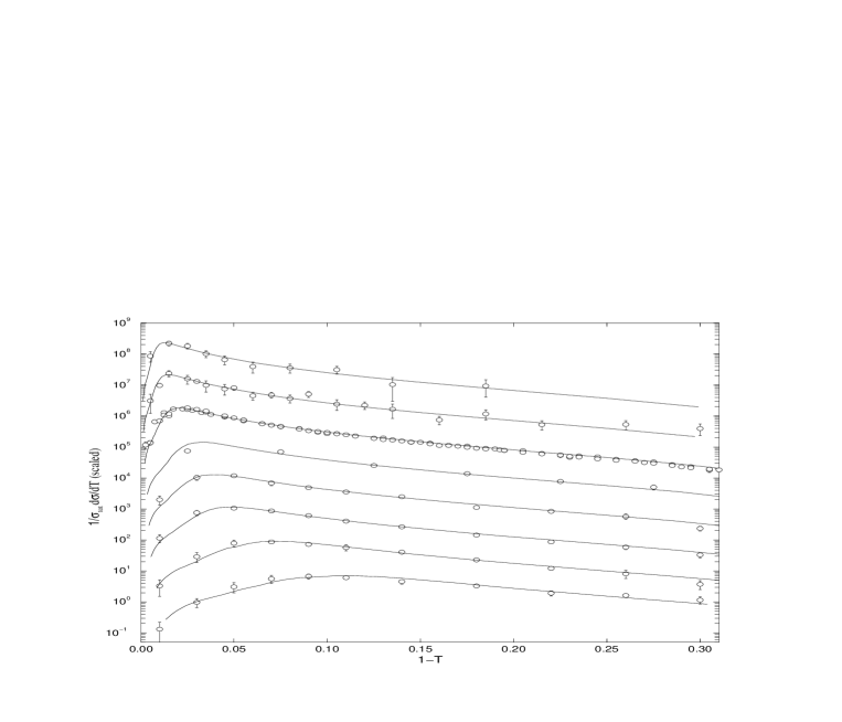
Figure 1: The comparison of the data with the QCD prediction for the thrust distribution at different energies (from bottom to top): $Q/{\rm GeV}=14,22,35,44,55,91,133,161,$ based on the shape function. The detailed description of the plot can be found in [10].

5 Summary

In this paper we have studied the power corrections to the differential thrust, $t=1-T$, and heavy mass, $\rho$, distributions in ${\rm e}^{+}{\rm e}^{-}$ annihilation close to the two-jet limit. In addressing this problem, we did not aim to justify a particular QCD-inspired phenomenological model, but rather to formulate a framework with which to study the relationship between perturbative and nonperturbative effects in high-energy final states. We have seen that, despite the fact that the thrust and heavy jet mass are not inclusive quantities, the leading nonperturbative corrections to their differential distributions can be factorized into the perturbative and nonperturbative functions, in much the same way as for inclusive cross sections. We identified nonperturbative infrared shape functions that organize all leading power corrections, $1/(tQ)^{n}$ and $1/(\rho Q)^{n}$. Although not universal themselves, these shape functions can be derived from universal matrix elements that describe energy flow. We anticipate that it will be possible to extend these considerations to a wide class of infrared safe event shapes and hard-scattering processes.

Acknowledgements

We are grateful to Hasko Stenzel for useful correspondence. This was supported in part by the EU Fourth Framework Programme “Training and Mobility of Researchers”, Network “Quantum Chromodynamics and the Deep Structure of Elementary Particles”, contract FMRX–CT98–0194 (DG 12 – MIHT) and by the National Science Foundation, grant PHY9722101.

References

-
[1]
S. Bethke, hep-ex/9812026;
S. Hahn, DELPHI 98-174 hep-ex/9812021;
P.A. Movilla Fernandez et al., hep-ex/9807007. -
[2]
DELPHI Coll., Z. Phys. C73 (1997) 22;
ALEPH Coll., Contribution to EPS-HEP97, Jerusalem 19-26 Aug. 1997, abstract 610.
D. Wicke, Nucl. Phys. Proc. Suppl. 64 (1998) 27.
P.A. Movilla Fernandez, et. al. and the JADE Coll., Eur. Phys. J. C1 (1998) 461.
O. Biebel, Nucl. Phys. B, Proc. Suppl. 64 (1998) 22. -
[3]
B.R. Webber, Phys. Lett. B339 (1994) 148;
Yu.L. Dokshitzer and B.R. Webber, Phys. Lett. B352 (1995) 451. - [4] G.P. Korchemsky and G.Sterman, Nucl. Phys. B437 (1995) 415.
- [5] R. Akhoury and V. Zakharov, Phys. Lett. B357 (1995) 646; Nucl. Phys. B465 (1996) 295.
- [6] M. Beneke and V.M. Braun, Nucl. Phys. B454 (1995) 253.
- [7] G.P. Korchemsky and G. Sterman, in proceedings of the 30th Rencontres de Moriond, QCD and High Energy Hadronic Interactions, Les Arcs, Savoie, France, 18-25 March, 1995, ed. J. Tran Thanh Van (Editions Frontieres, Gif-sur-Yvette, 1995), p.383; hep-ph/9505391.
- [8] Yu.L. Dokshitzer, G. Marchesini and B.R. Webber, Nucl. Phys. B469 (1996) 93.
- [9] Yu.L. Dokshitzer, A. Lucenti, G. Marchesini and G.P. Salam, Nucl. Phys. B511 (1998) 396; J. High Energy Phys. 5 (1998) 3.
- [10] G.P. Korchemsky, in proceedings of the 33th Rencontres de Moriond, QCD and High Energy Hadronic Interactions, Les Arcs, Savoie, France, March 21-28, 1998; hep-ph/9806537.
- [11] G.P. Korchemsky and G. Sterman, Phys. Lett. B340 (1994) 96; R.D. Dikeman, M. Shifman and N.G. Uraltsev, Int. J. Mod. Phys. A11 (1996) 571; A.L. Kagan and M. Neubert, hep-ph/9805303.
-
[12]
N.A. Sveshnikov and F.V. Tkachev, Phys. Lett. B382 (1996) 403;
P.S. Cherzor and N.A. Sveshnikov, hep-ph/9710349. - [13] G.P. Korchemsky, G. Oderda and G. Sterman, in proceedings of the 5th International Workshop “Deep Inelastic Scattering and QCD”, ed. J. Repond and D. Krakauer, AIP Conf. Proc. No.407, Woodbury, NY, 1997, p.988; hep-ph/9708346.
- [14] M. Testa, J. High Energy Phys. 6 (1998) 9809.
- [15] Yu.L. Dokshitzer and B.R. Webber, Phys. Lett. B 404 (1997) 321.
- [16] S. Catani, L. Trentadue, G. Turnock and B.R. Webber, Nucl. Phys. B407 (1993) 3.
- [17] J.C. Collins, D.E. Soper and G. Sterman, in Perturbative Quantum Chromodynamics, ed. A.H. Mueller (World Scientific, Singapore, 1989), p. 1.
- [18] P. Nason and M.H. Seymour, Nucl. Phys. B454 (1995) 291.
-
[19]
J.G.M. Gatheral, Phys. Lett. 133B (1984) 90;
J. Frenkel and J.C. Taylor, Nucl. Phys. B246 (1984) 231. - [20] H. Contopanagos, E. Laenen and G. Sterman, Nucl. Phys. B484 (1997) 303.
- [21] F.R. Ore and G. Sterman, Nucl. Phys. B165 (1980) 93.
- [22] G.P. Korchemsky and G. Marchesini, Nucl. Phys. B406 (1993) 225; Phys. Lett. B313 (1993) 433.
- [23] H. Stenzel, private communication.