hep-ph/9902290

Infrared Quasi Fixed Points and Mass Predictions in the MSSM II: Large $\tan\beta$ Scenario

M.  Jurčišin and D. I. Kazakov

Bogoliubov Laboratory of Theoretical Physics, Joint Institute for Nuclear Research,
141 980 Dubna, Moscow Region, Russian Federation

1 Introduction

Supersymmetric extensions of the Standard Model (SM) are believed to be the most promising theories at high energies. An attractive feature of SUSY theories is a possibility of unifying various forces of Nature. The best known supersymmetric extension of the SM is the so-called Minimal Supersymmetric Standard Model (MSSM) [1]. The parameter freedom of the MSSM comes mainly from the so-called soft SUSY breaking terms, which are the sources of uncertainty in the MSSM predictions. The most common way to reduce this uncertainty is to assume universality of soft terms, which means an equality of some parameters at a high energy scale. Adopting the universality, one reduces the parameter space to a five-dimensional one [1]: $m_{0}$, $m_{1/2}$, $A$, $\mu$, and $B$. The last two parameters it is convenient to trade for the electroweak scale $v^{2}=v_{1}^{2}+v_{2}^{2}=(174.1GeV)^{2}$, and $\tan\beta=v_{2}/v_{1}$, where $v_{1}$ and $v_{2}$ are the Higgs field vacuum expectation values. In papers [3]-[15] further reduction of the parameter space has been discussed based on the concept of the so-called infrared quasi fixed points (IRQFP) [16, 17], which shows insensitivity of some low-energy MSSM parameters to their initial high energy values. This opens a possibility to compute physical values of some masses and soft couplings at low-energies without detailed knowledge of physics at high energies. For example, in Ref. [5] the dependence of sparticle spectrum on two free parameters, namely $m_{0}$ and $m{1/2}$, has been discussed. In paper [15] we argue that for some sparticles and Higgs bosons it is possible to reduce this two-dimensional parameter space into one-dimensional one using the IRQFPs. The only relevant parameter is $m_{1/2}$ which is directly related to gluino mass $M_{3}$.

In the literature the IRQFP scenario has been considered in detail mainly for the MSSM in the low $\tan\beta$ regime. In the present paper we make an analysis similar to that in Ref.[15] but for large $\tan\beta$. In this case the reduction of the parameter space is also possible and the IRQFPs also appear. The situation, however, is more complicated because now we have the whole set of Yukawa couplings of the third generation and the corresponding soft trilinear terms. Here no exact solution of the renormalization group equations (RGEs) is known and one is bound to a numerical investigation. Nevertheless, we show that the IRQFP are well pronounced and may be used to calculate a mass spectrum.

In what follows we assume the equality of all three Yukawa couplings at the GUT scale, i.e. we work in the so-called $SO(10)$ unification scheme which is natural for large $\tan\beta$. The other possibility, $h_{t}\approx h_{b}>h_{\tau}$, is not considered here. We use the obtained IRQFPs to make predictions for the Higgs masses and masses of the stops and sbottoms as functions of the only free parameter, namely the gluino mass, $M_{3}$. We also present the mass of the lightest Higgs boson as a function of the geometric mean of stop masses, sometimes called $M_{SUSY}$, and confront our results with the experimental data on SUSY and Higgs boson searches.

The paper is organized as follows. In Section 2 we present the numerical analysis of the RGE’s and demonstrate their infrared behaviour. IRQFPs are found and used in Section 3 to obtain the mass spectrum of Higgs bosons and some SUSY particles. In Section 4 we discuss our main results and conclusions.

2 Infrared Quasi Fixed Points and RGE’s

We now give a short description of the infrared behaviour of the RGE’s in the MSSM for the large $\tan\beta$ regime. We follow the same strategy as in our previous paper [15] related to the low $\tan\beta$ case, though the analysis for large $\tan\beta$ is more complicated because one has to take into account three Yukawa couplings, $Y_{i}$, where $Y_{i}=h_{i}^{2}/(4\pi)^{2}$ and $i=(t,b,\tau)$ ($t$ corresponds to top-quark, $b$ to bottom-quark and $\tau$ to $\tau$-lepton) and the corresponding three trilinear SUSY breaking parameters $A_{i}$. Since the analytical solution of the RGE’s is unknown (some semianalytical solutions for appropriate combinations of the parameters exist [18] but they are almost irrelevant for our analysis), we use numerical methods.

Recently it has been proven [19] that in the asymptotically free case the existence of stable IR fixed points for the Yukawa couplings implies stable IR fixed points for A-parameters and soft scalar masses. (It follows also from superfield description of softly broken SUSY theories [20].) Thus, though we are not able to make an analytical analysis as has been done in Ref.[15], we can solve RGE’s numerically and find infrared fixed points. Here the same concept of IRQFP arises and one can find the intervals in which initial parameters can vary to be attracted by these fixed points.

We begin with an analysis of RGE’s for the Yukawa couplings. It is a self-consistent system of differential equations (together with well-known RGE’s for gauge couplings), which in the one-loop order has the following form (see e.g. Ref.[2]):

$$\frac{dY_{t}}{dt} = Y_{t}\left(\frac{16}{3}\tilde{\alpha}_{3}+3\tilde{\alpha}_{2}+\frac{13}{15}\tilde{\alpha}_{1}-6Y_{t}-Y_{b}\right)\,,$$ (1)

$$\frac{dY_{b}}{dt} = Y_{b}\left(\frac{16}{3}\tilde{\alpha}_{3}+3\tilde{\alpha}_{2}+\frac{7}{15}\tilde{\alpha}_{1}-Y_{t}-6Y_{b}-Y_{\tau}\right)\,,$$ (2)

$$\frac{dY_{\tau}}{dt} = Y_{\tau}\left(3\tilde{\alpha}_{2}+\frac{9}{5}\tilde{\alpha}_{1}-3Y_{b}-4Y_{\tau}\right)\,,$$ (3)

where $\tilde{\alpha}_{i}=\alpha_{i}/(4\pi)$, $t=\log(M_{GUT}^{2}/Q^{2})$. As it has been mentioned in the introduction we assume the equality of the Yukawa couplings of the third generation at the GUT scale ($M_{GUT}=10^{16}$ GeV): $Y_{t}(M_{GUT})=Y_{b}(M_{GUT})=Y_{\tau}(M_{GUT})$.

In Figs. 1a,b,c the numerical solutions of the RGE’s are shown for a wide range of initial values of $\rho_{t}(M_{GUT})=\rho_{b}(M_{GUT})=\rho_{\tau}(M_{GUT})$ from the interval $<0.2,5>$, where $\rho_{i}=Y_{i}/\tilde{\alpha}_{3}$. As one can see from this figure, there is a strong restriction on all the Yukawa couplings at the scale $M_{Z}$. One can also clearly see the IRQFP type behaviour when the parameter $\rho_{i}$ is big enough. Further restrictions on the initial values, which follow from the phenomenological arguments, are considered in the next section.

We have found the following values of the Yukawa couplings $h_{i}$ at the $M_{Z}$ scale

$$h_{t}\in<0.787,1.048>,\ \ h_{b}\in<0.758,0.98>,\ \ \ h_{tau}\in<0.375,0.619>.$$

Comparing $h_{t}$ and $h_{b}$ one can see that the ratio $h_{t}/h_{b}$ belongs to a very narrow interval $h_{t}/h_{b}\in<1.039,1.069>$. This property of stability helps us to determine $\tan\beta$ in the next section.

Now we proceed with the discussion of RGE’s for trilinear scalar couplings, $A_{i},i=(t,b,\tau)$. The one-loop RGE’s have the following form (see e.g. Ref.[2]):

$$\frac{dA_{t}}{dt} = -\left(\frac{16}{3}\tilde{\alpha}_{3}M_{3}+3\tilde{\alpha}_{2}M_{2}+\frac{13}{15}\tilde{\alpha}_{1}M_{1}\right)-6Y_{t}A_{t}-Y_{b}A_{b}\,,$$ (4)

$$\frac{dA_{b}}{dt} = -\left(\frac{16}{3}\tilde{\alpha}_{3}M_{3}+3\tilde{\alpha}_{2}M_{2}+\frac{7}{15}\tilde{\alpha}_{1}M_{1}\right)-6Y_{b}A_{b}-Y_{t}A_{t}-Y_{\tau}A_{\tau}\,,$$ (5)

$$\frac{dA_{\tau}}{dt} = -\left(3\tilde{\alpha}_{2}M_{2}+\frac{9}{5}\tilde{\alpha}_{1}M_{1}\right)-3Y_{b}A_{b}-4Y_{\tau}A_{\tau}\,,$$ (6)

$$\frac{dM_{i}}{dt} = -b_{i}\tilde{\alpha}_{i}^{2}M_{i}\,,$$ (7)

where $M_{i}$ are the gaugino masses, $b_{i}$ are the one-loop $\beta$-function coefficients for the gauge couplings $\tilde{\alpha}_{i}$ with $(b_{1},b_{2},b_{3})=(33/5,1,-3)$. This system of RGE’s together with the equations for the Yukawa couplings (1-3) is self-consistent, and we solve it numerically. The results are shown in Figs. 1d,e for the following quantities $\rho_{A_{i}}=A_{i}/M_{3},i=(t,b)$ for different initial values at the GUT scale and for $\rho_{i}(M_{GUT})=5$. One can see the strong attraction to the fixed points.

The question of stability of these IRQFPs becomes important for further consideration. We have analyzed their stability under the change of the initial conditions for $\rho_{i}(M_{GUT})$ and have found remarkable stability, which allows one to use them as fixed parameters at the $M_{Z}$ scale. In Fig. 1f a particular example of stability of IRQFP for $A_{t}$ is shown. As a result we have the following IRQFP values for the parameters $\rho_{A_{i}}$:

$$\rho_{A_{t}}\approx-0.619,\ \ \rho_{A_{b}}\approx-0.658,\ \ \rho_{A_{\tau}}\approx 0.090.$$

The last value for $A_{\tau}$ is not important for calculation of masses (see the next section).

The last step in the investigation of the RGE’s is the calculation of the soft mass parameters and finding of appropriate IRQFPs. The one-loop RGE’s for the masses are (see e.g. Ref.[2])

$$\frac{dm_{Q}^{2}}{dt} = \left(\frac{16}{3}\tilde{\alpha}_{3}M_{3}^{2}+3\tilde{\alpha}_{2}M_{2}^{2}+\frac{1}{15}\tilde{\alpha}_{1}M_{1}^{2}\right)-Y_{t}\left(m_{Q}^{2}+m_{U}^{2}+m_{H_{2}}^{2}+A_{t}^{2}\right)$$ (8)

$$- Y_{b}\left(m_{Q}^{2}+m_{D}^{2}+m_{H_{1}}^{2}+A_{b}^{2}\right)\,,$$

$$\frac{dm_{U}^{2}}{dt} = \left(\frac{16}{3}\tilde{\alpha}_{3}M_{3}^{2}+\frac{16}{15}\tilde{\alpha}_{1}M_{1}^{2}\right)-2Y_{t}\left(m_{Q}^{2}+m_{U}^{2}+m_{H_{2}}^{2}+A_{t}^{2}\right)\,,$$ (9)

$$\frac{dm_{D}^{2}}{dt} = \left(\frac{16}{3}\tilde{\alpha}_{3}M_{3}^{2}+\frac{4}{15}\tilde{\alpha}_{1}M_{1}^{2}\right)-2Y_{b}\left(m_{Q}^{2}+m_{D}^{2}+m_{H_{1}}^{2}+A_{b}^{2}\right)\,,$$ (10)

$$\frac{dm_{H_{1}}^{2}}{dt} = 3\left(\tilde{\alpha}_{2}M_{2}^{2}+\frac{1}{5}\tilde{\alpha}_{1}M_{1}^{2}\right)-3Y_{b}\left(m_{Q}^{2}+m_{D}^{2}+m_{H_{1}}^{2}+A_{b}^{2}\right)$$ (11)

$$- Y_{\tau}\left(m_{L}^{2}+m_{E}^{2}+m_{H_{1}}^{2}+A_{\tau}^{2}\right)\,,$$

$$\frac{dm_{H_{2}}^{2}}{dt} = 3\left(\tilde{\alpha}_{2}M_{2}^{2}+\frac{1}{5}\tilde{\alpha}_{1}M_{1}^{2}\right)-3Y_{t}\left(m_{Q}^{2}+m_{U}^{2}+m_{H_{2}}^{2}+A_{t}^{2}\right)\,,$$ (12)

$$\frac{dm_{L}^{2}}{dt} = 3\left(\tilde{\alpha}_{2}M_{2}^{2}+\frac{1}{5}\tilde{\alpha}_{1}M_{1}^{2}\right)-Y_{\tau}\left(m_{L}^{2}+m_{E}^{2}+m_{H_{1}}^{2}+A_{\tau}^{2}\right)\,,$$ (13)

$$\frac{dm_{E}^{2}}{dt} = \frac{12}{5}\tilde{\alpha}_{1}M_{1}^{2}-2Y_{\tau}\left(m_{L}^{2}+m_{E}^{2}+m_{H_{1}}^{2}+A_{\tau}^{2}\right)\,,$$ (14)

where $m_{H_{1}}^{2}$ and $m_{H_{2}}^{2}$ are the SUSY breaking masses from the Higgs potential, $m_{Q}^{2}$, $m_{U}^{2}$ and $m_{D}^{2}$ are the squark masses (here $Q$ refers to the third generation squark doublet, $U$ to the stop singlet and $D$ to the sbottom singlet) and $m_{L}^{2}$ and $m_{E}^{2}$ are the slepton masses ($L$ refers to the third generation doublet and $E$ to the stau singlet). We can express them (as in the case of trilinear soft couplings $A_{i}$) via the common gaugino mass $m_{1/2}$ or, equivalently, via the gluino mass $M_{3}=(\tilde{\alpha}_{3}/\tilde{\alpha}_{0})m_{1/2}$, when investigating their IR fixed point behaviour.

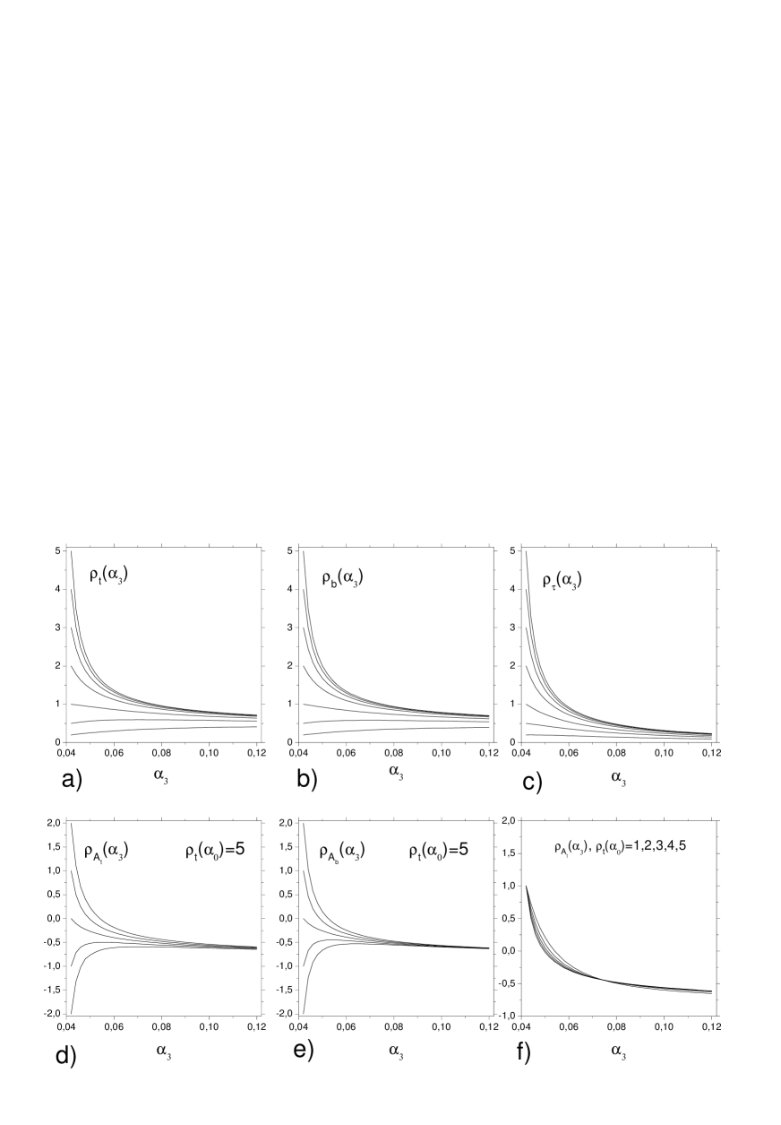
Figure 1: The infrared quasi fixed points for $\rho_{i}=Y_{i}/\tilde{\alpha}_{3}$ $i=t,b,\tau$ (a,b,c), $\rho_{A_{i}}=A_{i}/M_{3}$ $i=t,b$ (d,e) and $\rho_{A_{t}}$ with $\rho_{A_{t}}(\alpha_{0})=1$ for different initial values of $\rho_{t}(\alpha_{0})$ (f).

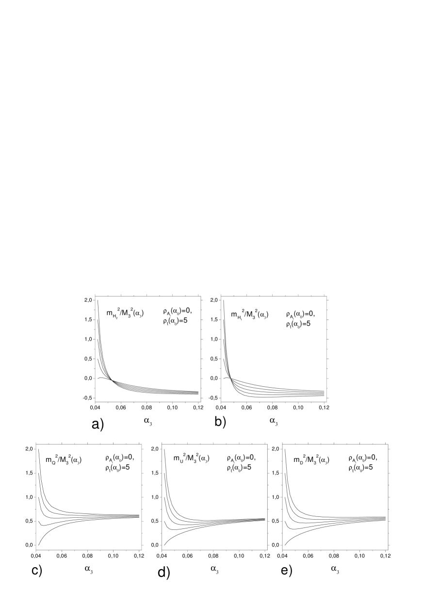
Figure 2: The infrared quasi fixed points for mass parameters.

In contrast with the low $\tan\beta$ MSSM scenario, where there is no obvious infrared attractive fixed point for $m_{H_{1}}^{2}$, for large $\tan\beta$ it has almost the same infrared behaviour as $m_{H_{2}}^{2}$ because of the non-negligible bottom-quark Yukawa coupling in the corresponding RGE. One can see in Figs. 2a,b that both the ratios $m_{H_{1}}^{2}/M_{3}^{2}$ and $m_{H_{2}}^{2}/M_{3}^{2}$ are negative in the infrared region. This requires a proper value of the parameter $\mu$ for the electro-weak symmetry breaking to take place.

As one can see from Figs. 2a,b, there exist IRQFP’s

$$m_{H_{1}}^{2}/M_{3}^{2}\approx-0.306\ \ m_{H_{2}}^{2}/M_{3}^{2}\approx-0.339,$$

The numbers correspond to the initial condition $m_{0}^{2}/m_{1/2}^{2}=0$. When calculating the mass of the Higgs bosons one has to take into account small deviation from these fixed points. Later on we consider initial values for the ratio $m_{0}^{2}/m_{1/2}^{2}$ belonging to the following interval $m_{0}^{2}/m_{1/2}^{2}\in<0,2>$.

In Figs. 2c,d,e the infrared behaviour of the soft SUSY breaking squark masses is shown. One can immediately see that all masses have IRQFPs which we use in the next section to find the mass spectrum. For further analysis only the squark masses are important. As for sleptons they also have an attractive infrared behaviour but it does not influence the mass spectrum of the Higgs bosons and we do not show them explicitly.

Numerical values of the ratios are the following:

$$m_{Q}^{2}/M_{3}^{2}\approx 0.58,\ \ m_{U}^{2}/M_{3}^{2}\approx 0.52,\ \ m_{D}^{2}/M_{3}^{2}\approx 0.53,$$

obtained for $m_{0}^{2}/m_{1/2}^{2}=0$. One can refer to them as to IRQFPs. Small deviations from these fixed points are again taken into account when we calculate the mass spectrum of the Higgs bosons. To do this we again address the question of stability of these IRQFPs. Solving the RGE’s for different initial values of the Yukawa couplings, one again finds a very week dependence on them.

We have analyzed also the behaviour of the bilinear SUSY breaking parameter $B$. The situation here is the same as in low $\tan\beta$ case. The ratio $B/M_{3}$ does not exhibit the infrared quasi fixed point behaviour and so we do not use it in further discussion.

Thus, one can see that solutions of RGE’s for all MSSM SUSY breaking parameters (the only exception is the parameter $B$) are driven to the infrared attractive fixed points if the Yukawa couplings at the GUT scale are large enough. In the next section we use the obtained IRQFPs to calculate the masses of some particles of interest.

Our analysis is constrained by the one-loop RG equations. On the other hand Abel and Allanach [14] have studied the two-loop RGEs in the low $\tan\beta$ case. The difference between one-loop and two-loop IRQFPs is around 10 per cent. At the same time the deviations from the IRQFPs obtained by one-loop RGEs are also around 10-15 per cent. However, as we show in the next section (see Fig.3,4), these deviations give negligible corrections to the Higgs boson masses. For this reason and in order to make our arguments simple and clear we follow the strategy described in Ref.[15] and consider only one-loop RG equations to determine the IRQFPs.

3 Masses of Stops, Sbottoms and Higgs Bosons

In this section we use the obtained restrictions on the parameter space coming from the IRQFP behaviour for the computation of the masses of the Higgs bosons, stops and sbottoms.

We begin with the description of our strategy. As input parameters we take the known values of the top-quark, bottom-quark and $\tau$-lepton masses ($m_{t},m_{b},m_{\tau}$), the experimental values of the gauge couplings [21] $\alpha_{3}=0.12,\alpha_{2}=0.034,\alpha_{1}=0.017$, the sum of Higgs vev’s squared $v^{2}=v_{1}^{2}+v_{2}^{2}=(174.1GeV)^{2}$ and the IRQFPs obtained in the previous section. First, we use the well-known relations between the running quark and lepton masses and the Higgs v.e.v.s in the MSSM

$$m_{t} = h_{t}v\sin\beta\,,$$ (15)

$$m_{b} = h_{b}v\cos\beta\,,$$ (16)

$$m_{\tau} = h_{\tau}v\cos\beta\,.$$ (17)

One can use one of these equations or some combination of them for determination of the value of $\tan\beta$. As has been shown in the previous section the ratio $h_{t}/h_{b}$ is almost constant in the range of possible values of $h_{t}$ and $h_{b}$. This opens a possibility to determine the value of $\tan\beta$, which depends only on the running masses $m_{t}$ and $m_{b}$ and very weakly on the Yukawa couplings $h_{t}$ and $h_{b}$. Thus, we use the following relation for $\tan\beta$:

$$\tan\beta=\frac{m_{t}}{m_{b}}\frac{h_{b}}{h_{t}}\,.$$ (18)

First, we determine $\tan\beta$ using the QCD-corrections to the running top-quark and bottom-quark masses (see below). Then, we apply this value for calculation of all needed quantities to determine the SUSY corrections to these masses, which are again used as input parameters for evaluation of corrections to $\tan\beta$. After such procedure we are able to obtain a stable value for $\tan\beta$.

As has been mentioned above, for the evaluation of $\tan\beta$ we first need to determine the running top- and bottom-quark masses. We find them using the well-known relations to the pole masses (see e.g. [12, 22, 23]). We begin with the top-quark running mass which is given by the following relation:

$$m_{t}(m_{t})=\frac{m_{t}^{pole}}{1+\left(\frac{\Delta m_{t}}{m_{t}}\right)_{QCD}+\left(\frac{\Delta m_{t}}{m_{t}}\right)_{SUSY}},$$ (19)

where $m_{t}^{pole}=(174.1\pm 5.4)$ GeV [24]. Eq.(19) includes the QCD gluon correction (in the $\overline{MS}$ scheme)

$$\left(\frac{\Delta m_{t}}{m_{t}}\right)_{QCD}=\frac{4\alpha_{3}}{3\pi}+10.92\left(\frac{\alpha_{3}}{\pi}\right)^{2}\,,$$ (20)

and the stop/gluino correction [23]

$$\left(\frac{\Delta m_{t}}{m_{t}}\right)_{SUSY}= - \frac{g_{3}^{2}}{12\pi^{2}}\Bigl{\{}B_{1}(m_{t},M_{3},\tilde{m}_{t_{1}})+B_{1}(m_{t},M_{3},\tilde{m}_{t_{2}})$$ (21)

$$- \sin(2\theta_{t})\frac{M_{3}}{m_{t}}\left[B_{0}(m_{t},M_{3},\tilde{m}_{t_{2}})-B_{0}(m_{t},M_{3},\tilde{m}_{t_{1}})\right]\Bigr{\}},$$

where $\theta_{t}$ is the stop mixing angle, $\tilde{m}_{t_{1}}<\tilde{m}_{t_{2}}$, and

$$B_{n}(m_{t},m_{1},m_{2})=-\int_{0}^{1}dx\,x^{n}\ln\left[\frac{(1-x)m_{1}^{2}+xm_{2}^{2}-x(1-x)p^{2}}{m_{t}^{2}}\right].$$ (22)

We use the following procedure to evaluate the running top mass. First, we take into account only the QCD correction and find $m_{t}(m_{t})$ at the first approximation. This allows us to determine both the stop masses and the stop mixing angle. Next, having at hand the stop and gluino masses, we take into account the stop/gluino corrections. The results are given in the table below.

Now we consider the bottom-quark running mass at the $M_{Z}$ scale, $m_{b}(M_{Z})$. The situation is more complicated because the mass of the bottom $m_{b}$ is essentially smaller than the scale $M_{Z}$ and so we have to take into account the running of this mass from $m_{b}$ scale to $M_{Z}$ scale. The procedure is the following [23, 25, 26]: we start with the bottom-quark pole mass, $m_{b}^{pole}=4.94\pm 0.15$ [27]. Then we find the SM $\overline{MS}$ bottom-quark mass at the $m_{b}$ scale using the two-loop $QCD$ corrections

$$m_{b}(m_{b})^{SM}=\frac{m_{b}^{pole}}{1+\left(\frac{\Delta m_{b}}{m_{b}}\right)_{QCD}}\,,$$ (23)

where [23, 26]

$$\left(\frac{\Delta m_{b}}{m_{b}}\right)_{QCD}=\frac{4\alpha_{3}(m_{b})}{3\pi}+12.4\left(\frac{\alpha_{3}(m_{b})}{\pi}\right)^{2}\,,$$ (24)

and $\alpha_{3}(m_{b})$ is the five-flavour three-loop running $\overline{MS}$ coupling. Then, we evolve this mass to the scale $M_{Z}$ using a numerical solution of the two-loop (together with three-loop $O(\alpha_{3}^{3})$) SM RGE’s [23, 25]. Taking $\alpha_{3}(M_{Z})=0.12$ one obtains $m_{b}(M_{Z})_{SM}=2.91$GeV. Using this value we can now calculate sbottom masses and then return back to take into account the SUSY corrections from massive SUSY particles

$$m_{b}(M_{Z})=\frac{m_{b}(M_{Z})^{SM}}{1+\left(\frac{\Delta m_{b}}{m_{b}}\right)_{SUSY}}\,.$$ (25)

We approximate these corrections by the sbottom/gluino and stop/chargino loops (for details see [23] and references therein):

$$\left(\frac{\Delta m_{b}}{m_{b}}\right)_{SUSY}=\left(\frac{\Delta m_{b}}{m_{b}}\right)_{\tilde{b}\tilde{g}}+\left(\frac{\Delta m_{b}}{m_{b}}\right)_{\tilde{t}\tilde{\chi}^{+}}\,.$$ (26)

The sbottom/gluino contribution is given by (21) with the substitution $t\to b$. The sbottom/chargino contribution is as follows (see [23] for details):

$$\left(\frac{\Delta m_{b}}{m_{b}}\right)_{\tilde{t}\tilde{\chi}^{+}} = -\frac{h_{t}^{2}}{16\pi^{2}}\mu\frac{A_{t}\tan\beta-\mu}{\tilde{m}_{t_{1}}^{2}-\tilde{m}_{t_{2}}^{2}}\left[B_{0}(0,\mu,\tilde{m}_{t_{2}})-B_{0}(0,\mu,\tilde{m}_{t_{1}})\right]$$ (27)

$$- \frac{g^{2}}{16\pi^{2}}\Bigl{\{}\frac{\mu M_{2}\tan\beta}{\mu^{2}-M_{2}^{2}}\left[c_{t}^{2}B_{0}(0,M_{2},\tilde{m}_{t_{2}})+s_{t}^{2}B_{0}(0,M_{2},\tilde{m}_{t_{1}})\right]$$

$$+ (\mu\leftrightarrow M_{2})\Bigr{\}}\,,$$

where $c_{t}$ $(s_{t})$ is $\cos\theta_{t}$ $(\sin\theta_{t})$.

The running bottom-quark mass slightly depends on the values of the top-quark Yukawa coupling and SUSY breaking parameters. Hence, we consider possible restrictions on these parameters. First, from eq.(15) we have a mathematical condition which requires $\sin\beta\leq 1$. It means that for the value of the running top-quark mass, $m_{t}$, we have to take only such values of the top-quark Yukawa coupling, $h_{t}$, that give $h_{t}\geq m_{t}/v$. This gives us a restriction from below for the top-quark Yukawa coupling. One can also impose a restriction from above. In what follows, we require the values of the top-quark, bottom-quark and $\tau$-lepton masses to be in appropriate experimental intervals. After analyzing the system of eqs.(15-17) one can see that the restriction from above for the Yukawa couplings follows from the mass of the $\tau$-lepton. This mass is very well defined experimentally ($m_{\tau}^{pole}=(1.7771\pm 0.0005)$GeV [28]) and to get a proper value one imposes the restriction on the values of the Yukawa couplings. Provided these two conditions are satisfied one has the following intervals for the third generation of Yukawa couplings:

$$h_{t}\in<0.988,1.069>,\ \ h_{b}\in<0.937,0.982>,\ \ h_{\tau}\in<0.537,0.670>\ \ \ \mbox{ for}\ \mu>0,$$

$$h_{t}\in<0.924,0.988>,\ \ h_{b}\in<0.882,0.937>,\ \ h_{\tau}\in<0.475,0.537>\ \ \ \mbox{for}\ \mu<0.$$

As one can see, the restriction is larger for the case of $\mu<0$. These values are obtained through the self-consistent procedure described above.

Now we can return back and compute the running bottom-quark masses in each boundary case. It is also possible to write down the corresponding values of $\tan\beta$ (see the table).

$\tan\beta$	$m_{t}(M_{Z})$	$m_{b}(M_{Z})$	$h_{t}$	$h_{b}$	$m_{0}^{2}/m_{1/2}^{2}$	$\mu$
76.4	186.1	2.24	1.069	0.982	0	$>0$
75.5	172.0	2.16	0.988	0.937	0	$>0$
77.3	186.2	2.21	1.069	0.982	2	$>0$
75.3	172.2	2.17	0.989	0.938	2	$>0$
44.9	172.0	3.63	0.988	0.937	0	$<0$
46.9	160.8	3.27	0.924	0.882	0	$<0$
45.3	172.1	3.60	0.989	0.938	2	$<0$
47.6	163.6	3.28	0.940	0.897	2	$<0$

Table 1: The values of $\tan\beta$ and running masses of the top and bottom quarks for both signs of the parameter $\mu$ and the ratio $m_{0}^{2}/m_{1/2}^{2}=0$ and 2 and for the upper (odd lines) and lower (even lines) values of top and bottom Yukawa couplings.

Due to the stop/gluino, bottom/gluino and stop/chargino corrections to the running top and bottom masses the predictions for $\tan\beta$ are different for different signs of $\mu$. As a consequence, the predictions for the Higgs bosons masses are also different in spite of the fact that these parameters are not explicitly dependent on the sign of $\mu$ at the tree level.

Now one may return to eqs.(15-17) to verify if the masses obtained correspond to the upper and lower experimental bounds. Indeed, there is a good agreement. In the table we give the masses of the top and bottom quarks obtained with the help of eqs.(15-16). The running masses which are calculated using eqs.(19,23,25) are inside the intervals given in the table for different signs of $\mu$ and the ratio $m_{0}^{2}/m_{1/2}^{2}$.

When calculating the stop and sbottom masses we need to know the Higgs mixing parameter $\mu$. For determination of this parameter we use the well-known relation between the $Z$-boson mass and the low-energy values of $m_{H_{1}}^{2}$ and $m_{H_{2}}^{2}$ which comes from the minimization of the Higgs potential:

$$\frac{M_{Z}^{2}}{2}+\mu^{2}=\frac{m_{H_{1}}^{2}+\Sigma_{1}-(m_{H_{2}}^{2}+\Sigma_{2})\tan^{2}\beta}{\tan^{2}\beta-1}\,,$$ (28)

where $\Sigma_{1}$ and $\Sigma_{2}$ are the one-loop corrections [29]. Large contributions to these functions come from stops and sbottoms. This equation allows one to obtain the absolute value of $\mu$. As has already been mentioned, the sign of $\mu$ remains a free parameter.

Having all the relevant parameters at hand we are now able to estimate the masses of phenomenologically interesting particles. With the fixed point type behaviour we have the only dependence left, namely on $m_{1/2}$ or the gluino mass, $M_{3}$. It is restricted only experimentally: $M_{3}>144$GeV [21] for arbitrary values of the squarks masses.

The stop and sbottom masses are determined by diagonalizing the corresponding mass matrix [30, 31]. The results are shown in Figs.3a,b. Since the masses are very heavy, the one-loop corrections to them are not important from the phenomenological point of view. For $M_{3}\approx 1.5$TeV (which corresponds to $m_{1/2}\approx 500$ GeV) we obtain the following numerical values for the squark masses:

$$\tilde{m}_{t_{1}}\approx 1041\ GeV,\ \tilde{m}_{t_{2}}\approx 1195\ GeV,\ \tilde{m}_{b_{1}}\approx 1050\ GeV,\ \tilde{m}_{b_{2}}\approx 1185\ GeV\ \ \mbox{for}\ \mu>0,$$

$$\tilde{m}_{t_{1}}\approx 1050\ GeV,\ \tilde{m}_{t_{2}}\approx 1218\ GeV,\ \tilde{m}_{b_{1}}\approx 1066\ GeV,\ \tilde{m}_{t_{1}}\approx 1196\ GeV\ \ \mbox{for}\ \mu<0.$$

The dependence of the squark masses on the allowed variation of the Yukawa couplings is negligible.

Much interest attracts the mass spectrum of the Higgs bosons. In the MSSM, after electroweak symmetry breaking, the Higgs sector consists of five physical states. Their masses obtain large radiative corrections. In contrast with the low $\tan\beta$ case, for high $\tan\beta$ they are important for all Higgs bosons and not only for the lightest one. For the charged bosons and CP-odd one it is sufficient to take into account the one-loop corrections. As for the lightest CP-even Higgs boson we also include the two-loop contributions. For this purpose we need the masses of the stops and sbottoms calculated above.

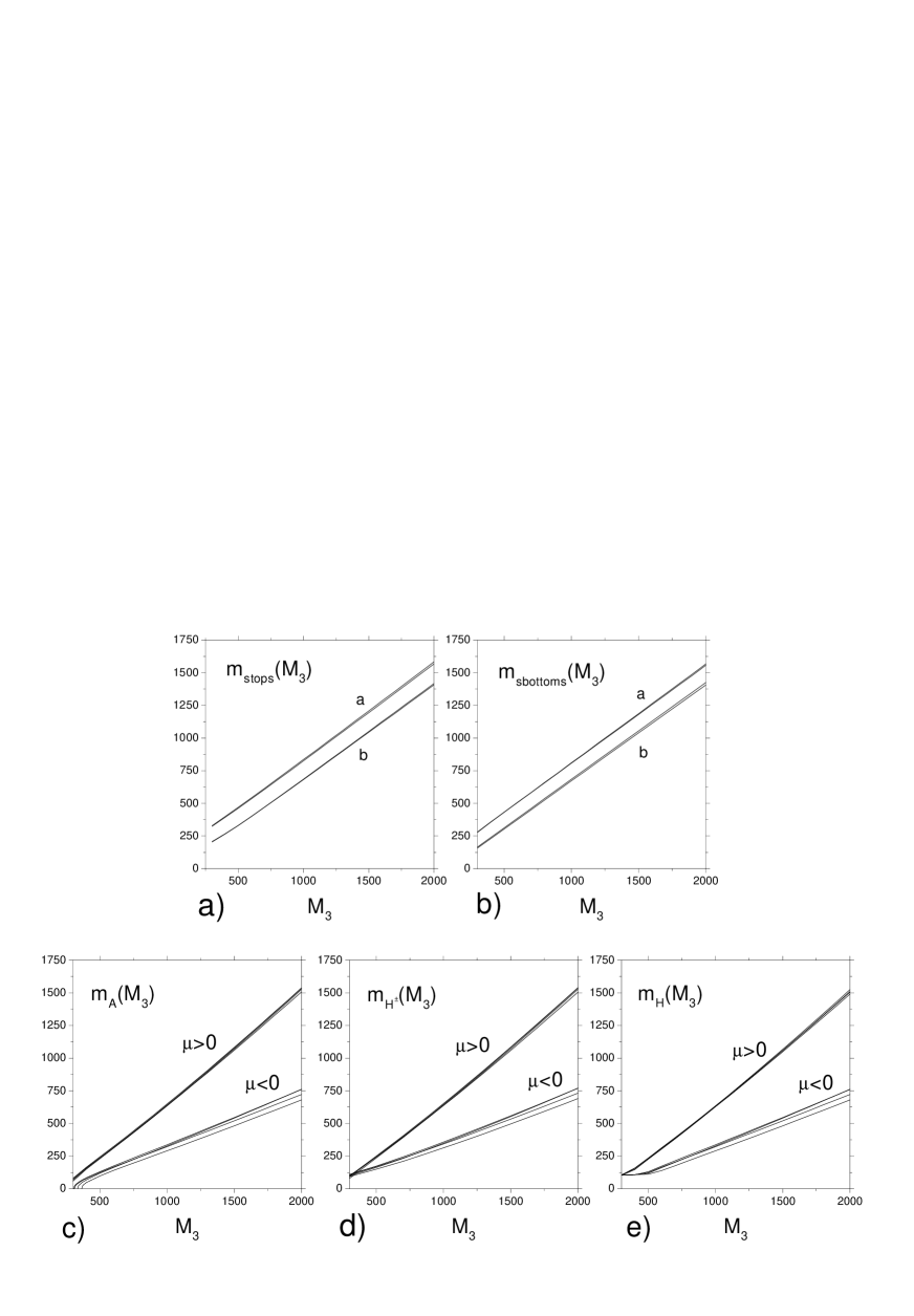
Figure 3: Masses of the stops a), sbottoms b) and Higgs bosons c),d),e) as functions of the gluino mass, $M_{3}$. The curves (a) in Figs. a) and b) correspond to $\tilde{m}_{t_{2}}$ and $\tilde{m}_{b_{2}}$ and the curves (b) correspond to $\tilde{m}_{t_{1}}$ and $\tilde{m}_{b_{1}}$ for both signs of $\mu$. Different lines for masses of the Higgs bosons in both the cases $\mu>0$ and $\mu<0$ are due to the deviations from the IRQFPs and from the uncertainty in the Yukawa couplings.

The one-loop corrected mass $M_{A}^{2}$ is given by the following equation [29]:

$$m_{A}^{2}=m_{H_{1}}^{2}+m_{H_{2}}^{2}+2\mu^{2}+\Sigma_{1}+\Sigma_{2}+\frac{\Delta}{\sin 2\beta}\,.$$ (29)

Following our strategy and using the IRQFPs obtained above we have the value of $m_{A}$ which depends only on the gluino mass $M_{3}$ shown in Fig.3c. One can see that the requirement of positivity of $m_{A}^{2}$ excludes the region with small $M_{3}$. This restriction is important when analyzing the lightest Higgs boson mass. In the most promising region $M_{3}>1$ TeV ($m_{1/2}>300$ GeV), however, for the both cases $\mu>0$ and $\mu<0$ the mass of the CP-odd Higgs boson is too heavy to be detected in the near future

$$m_{A}>1100\ \mbox{GeV for}\ \ \mu>0,\ \ \ m_{A}>570\ \mbox{GeV for}\ \ \mu<0,$$

when $M_{3}\approx 1.5$TeV.

The mass of the charged Higgs bosons $m_{H^{\pm}}^{2}$ with one-loop corrections can be written as follows [32]:

$$m_{H^{\pm}}^{2}=m_{A}^{2}+M_{W}^{2}+\Delta_{c}^{2}\,.\\$$ (30)

In Fig.3d one can see its behaviour for different signs of $\mu$. Like in the case of low $\tan\beta$ the charged Higgses are heavy but there is a big difference between the cases with $\mu>0$ and $\mu<0$. One can find the following values at the typical scale $M_{3}\approx 1.5$TeV:

$$m_{H^{\pm}}>1105\ \mbox{GeV for}\ \ \mu>0,\ \ \ m_{H^{\pm}}>575\ \mbox{GeV for}\ \ \mu<0.$$

The most phenomenologically interesting particle is the lightest Higgs boson $h$. The two-loop corrected masses of the CP-even Higgs bosons, $h$ and $H$ are given by

$$m_{H,h}^{2}=\frac{1}{2}(Tr(M^{2})\pm\sqrt{(Tr(M^{2}))^{2}-4\det(M^{2}))}\,,$$ (31)

where $M^{2}$ is the $2\times 2$ symmetric mass matrix given in Ref. [33]. One can see in Fig.3e that the heaviest CP-even Higgs boson, $H$, is too heavy for $\mu>0$ and not so heavy for $\mu<0$ but still far away from the range of the nearest experiments. For the typical value of the gluino mass $M_{3}\approx 1.5$ TeV its mass is

$$m_{H}>1100\ \mbox{GeV for}\ \ \mu>0,\ \ \ m_{H}>570\ \mbox{GeV for}\ \ \mu<0.$$

The dependence on the deviations from the IRQFPs is not relevant as one can see in Fig. 3e, and $H$-boson is too heavy to be detected in the near future.

The situation is different for the lightest Higgs boson, $h$, which is much lighter. As one can see from Fig.4 the deviations of the Yukawa couplings from their IRQFPs give rather wide interval of values for $m_{h}$ in both the cases $\mu>0$ and $\mu<0$. One has the following values of $m_{h}$ at a typical scale $M_{3}=1.5$TeV

$$m_{h} = 129.3-0.1-7.2\pm 5\ \mbox{GeV, for}\ \mu>0\,,$$

$$m_{h} = 121.8-0.3-4.1\pm 5\ \mbox{GeV, for}\ \mu<0\,.$$

The first uncertainty is connected with the deviations from the IRQFPs for mass parameters, the second one with the Yukawa coupling IRQFPs, and the third one is due to the experimental uncertainty in the top-quark mass. One can immediately see that the deviations from the IRQFPs for mass parameters are negligible and only influence the steep fall of the function on the left, which is related to the restriction on the CP-odd Higgs boson mass $m_{A}$. In contrast with the low $\tan\beta$ case, where the dependence on the deviations from the fixed points was about $1$ GeV, in the present case the dependence is much stronger. The experimental uncertainty in the strong coupling constant $\alpha_{s}$ is not included because it is negligable compared to those of the top-quark mass and the Yukawa couplings and is not important here contrary to the low $\tan\beta$ case (see Ref. [15]).

We show in Fig.4 the mass of the lightest Higgs boson as a function of $(\tilde{m}_{t_{1}}\tilde{m}_{t_{2}})^{1/2}$ which is usually referred to as the $M_{SUSY}$ scale. In this case we have the following values for the lightest Higgs boson for a typical value $M_{SUSY}=1$ TeV ($M_{3}\approx 1.3$TeV):

$$m_{h} = 128.2-0.4-7.1\pm 5\ \mbox{GeV, for}\ \mu>0\,,$$

$$m_{h} = 120.6-0.1-3.8\pm 5\ \mbox{GeV, for}\ \mu<0\,.$$

One can see that for large $\tan\beta$ scenario the masses of the lightest Higgs boson are typically around 120 GeV which is too heavy for observation at LEP II.

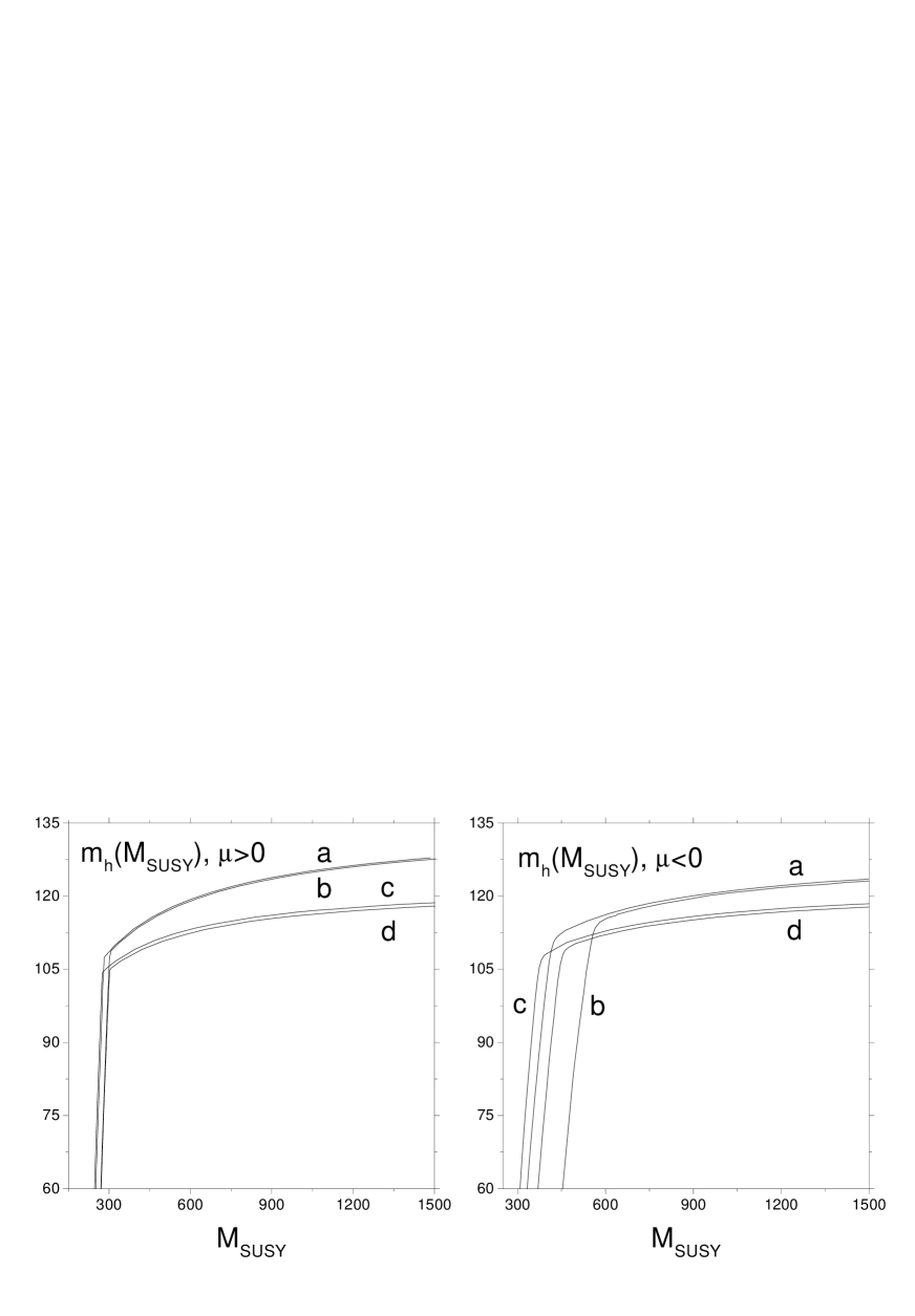
Figure 4: The mass of the lightest Higgs boson, $h$, as a function of $M_{SUSY}$ for different signs of $\mu$. The curves (a,b) correspond to the upper limit for the Yukawa couplings and $m_{0}^{2}/m_{1/2}^{2}=0$ (a) and $m_{0}^{2}/m_{1/2}^{2}=2$ (b). The curves (c,d) correspond to the lower limit for the Yukawa couplings and $m_{0}^{2}/m_{1/2}^{2}=0$ (c) and $m_{0}^{2}/m_{1/2}^{2}=2$ (d). The allowed values of the lightest Higgs boson mass lie inside the areas marked by these lines.

4 Summary and Conclusion

Thus, we have analyzed the fixed point behaviour of SUSY breaking parameters in the large $\tan{\beta}$ regime. We made this analysis assuming that the Yukawa couplings are initially large enough to be driven at infrared scales to their Hill-type quasi fixed points. This corresponds to a possible $SO(10)$ Grand Unification scenario with radiative EWSB.

We have found that solutions of RGE’s for some of the SUSY breaking parameters become insensitive to their initial values at unification scale. This is because at infrared scale they are driven to their IR quasi fixed points. These fixed points are used to make predictions for the masses of the Higgs bosons, stops and sbottoms. We have taken into account possible deviations from quasi IR fixed points. This leads to uncertainties in mass predictions which are much bigger than in the low $\tan\beta$ case, however, still dominated by the top mass experimental bounds.

In the IRQFP scenario all the Higgs bosons except for the lightest one are found to be too heavy to be accessible in the nearest experiments. The same is true for the stops and sbottoms. From this point of view the situation is the same as in the low $\tan\beta$ case and essentially coincides with the results of more sophisticated analyses [29]. The lightest neutral Higgs boson, contrary to the low $\tan\beta$ case, is not within the reach of LEPII leaving hopes for the Tevatron and LHC.

Acknowledgments

We are grateful to W. de Boer and G. K. Yeghiyan for useful discussions. Financial support from RFBR grants # 98-02-17453 and 96-15-96030 is kindly acknowledged.

References

-
[1]
H. P. Nilles, Phys. Rep. 110 (1984) 1,
H. E. Haber and G. L. Kane, Phys. Rep. 117 (1985) 75;
A.B. Lahanas and D.V. Nanopoulos, Phys. Rep. 145 (1987) 1;
R. Barbieri, Riv. Nuo. Cim. 11 (1988) 1; -
[2]
W. de Boer, Progr. in Nucl. and Particle Phys., 33
(1994) 201;
D.I. Kazakov, Surveys in High Energy Physics, 10 (1997) 153. - [3] M. Carena et al, Nucl. Phys. B419 (1994) 213.
- [4] W. Bardeen et al, Phys. Lett. B320 (1994) 110.
- [5] M. Carena and C.E.M. Wagner, Nucl. Phys. 452 (1995) 45.
- [6] V.Barger, M. S. Berger, P.Ohmann and R. J. N. Phillips, Phys. Lett. B314 (1993) 351.
- [7] P. Langacker and N. Polonsky, Phys. Rev. D50 (1994) 2199.
- [8] M. Lanzagorta and G.G. Ross, Phys.Lett. B349 (1995) 319.
-
[9]
J. Feng, N. Polonsky and S. Thomas, Phys. Lett. B370
(1996) 95,
N. Polonsky, Phys. Rev. D54 (1996) 4537. - [10] B. Brahmachari, Mod. Phys. Lett. A12 (1997) 1969.
- [11] P. Chankowski and S. Pokorski, Cern-TH-97-28, hep-ph/9702431, to appear in Perspectives on Higgs Physics II, edited by G.L. Kane (World Scientific, Singapure, 1998).
- [12] J. Casas, J. Espinosa, H. Haber, Nucl. Phys. B526 (1998) 3.
- [13] I. Jack, D.R.T. Jones and K.L. Roberts Nucl. Phys. B455 (1995) 83, P.M. Ferreira, I. Jack and D.R.T. Jones Phys. Lett. B357 (1995) 359.
- [14] S. A. Abel, B. C. Allanach Phys. Lett. B415 (1997) 371.
- [15] G. K. Yeghiyan, M. Jurčišin, D. I. Kazakov YERPHY-1520(20)-98, hep-ph/9807411.
-
[16]
C. T. Hill, Phys. Rev. D24 (1981) 691,
C. T. Hill, C. N. Leung, and S. Rao, Nucl. Phys. B262 (1985) 517. - [17] L.Ibanez and C. Lopez, Nucl.Phys. B233 (1984) 511.
-
[18]
E. G. Floratos, G. K. Leontaris, Nucl. Phys. B452 (1995) 471,
E.G. Floratos and G.K. Leontaris, Phys. Lett. B336 (1994) 194. - [19] I. Jack, and D. R. T. Jones, Phys. Lett. B443 (1998) 177.
- [20] D. I. Kazakov, hep-ph/9812513.
- [21] W. de Boer et al., hep-ph/9712376, Proc. of Int. Europhysics Conference on High Energy Physics (HEP 97), Jerusalem, Israel, August 1997.
- [22] B. Schrempp, M. Wimmer, Prog. Part. Nucl. Phys. 37 (1996) 1.
-
[23]
D. M. Pierce, J. A. Bagger, K. Matchev and R. Zhang,
Nucl. Phys. B491 (1997) 3,
J.A. Bagger, K. Matchev and D.M. Pierce, Phys. Lett. B348 (1995) 443. - [24] M. Jones, for the CDF and D0 Coll., talk at the XXXIIIrd Recontres de Moriond, (Electroweak Interactions and Unified Theories), Les Arcs, France, March 1998;
- [25] H.Arason, D. Castano, B. Keszthelyi, S. Mikaelian, E, Piard, P. Ramond, and B. Wright, Phys. Rev. D46 (1992) 3945.
- [26] N.Gray, D. J. Broadhurst, W. Grafe, and K. Schilcher, Z. Phys. C48 (1990) 673.
- [27] C. T. H. Davies, et al., Phys. Rev. D50 (1994) 6963.
- [28] Review of Particles Properties. Phys. Rev. D50 (1994).
- [29] A. V. Gladyshev, D. I. Kazakov, W. de Boer, G. Burkart, R. Ehret, Nucl. Phys. B498 (1997) 3.
- [30] L. Ibanez, C. Lopez, Phys. Lett B126 (1983) 54; Nucl. Phys. B233(1984) 511, Nucl. Phys. B256 (1985) 218.
- [31] W. de Boer, R. Ehret, D. Kazakov, Z. Phys. C67 (1995) 647.
- [32] A. Brignole, J. Ellis, G. Ridolfi and F. Zwirner, Phys. Lett. B271 (1991) 123.
- [33] M. Carena, M. Quiros, C.E.M. Wagner, Nucl. Phys. B461 (1996) 407.