Propagation of Gluons

From a Non-Perturbative Evolution Equation

in Axial Gauges

Abstract

We derive a non-perturbative evolution equation for the gluon propagator in axial gauges based on the framework of Wetterich’s formulation of the exact renormalization group. We obtain asymptotic solutions to this equation in the ultraviolet and infrared limits.

I INTRODUCTION AND SUMMARY

Non-Abelian gauge theories, and in particular QCD, are nowadays fairly well understood in the short-distance (large-momentum) regime where asymptotic freedom allows reliable calcuations within perturbation theory. On the other end of the scale, in the long-distance (low-momentum) domain, fundamental unanswered questions remain, linked intimately to the phenomenon of confinement (or the lack of detailed knowledge thereof), and posing severe infrared problems that present a tough challenge for developing adequate non-perturbative methods to perform practical calculations. Whereas the non-perturbative effects on QCD Green functions are small when all relevant momenta are large compared to the inverse confinement length, the properties of the vacuum, the dynamics of the QCD phase transition, or the formation of color-neutral hadronic excitations from colored quark and gluon fluctuations, are completely dominated by the non-perturbative infrared physics. Although lattice simulations provide to date the most rigorous non-perturbative studies of QCD, they suffer in one way or another from finite lattice size effects and violation of translational or rotational invariance. Moreover, the continuum limit of results obtained on a discrete Euclidean space lattice is a difficult problem itself.

A Average effective action and non-perturbative evolution equation

Therefore, it is clear that non-perturbative methods, formulated in continuous space and maintaining the symmetries of translations and rotations, are of fundamental need to complement insight into the infrared properties of QCD. Such a method has been developed [2, 3, 4] during the last few years and has found diverse applications [5, 6, 7]. It embodies the concept of the average effective action in continuous Euclidean or Minkowski space within the renormalization-group framework of quantum field theory. The basic idea is to study the theory within a volume $\Omega\propto 1/\kappa^{4}$ and effectively integrate out all quantum fluctuations that can be localized within that volume, i.e., fluctuations with squared momentum $q^{2}$ larger than $\kappa^{2}$. The average effective action $\overline{\Gamma}_{\kappa}$ is formulated as a functional integral over the microscopic quantum fields, and can be shown to be equal to the usual effective action $\Gamma$ for macroscopically averaged fields . The vacuum properties are obtained in the limit $\kappa\rightarrow 0$ where the volume $\Omega\propto 1/\kappa^{4}$ tends to infinity. In this paper, however, we are interested in the non-perturbative infrared behavior of gluons propagating in an unconfined quarkless world. The volume of such an idealized colored world cannot, of course, be infinite, since in reality confinement limits it to be of the size of a hadronic state $\Omega\,\sim 1$ fm³. Hence, as we ignore the existence of the QCD phase transition between the colored and the hadronic world, we must cut out the long-distance hadronic physics beyond distances of order 1 fm, and need to restrict $\kappa$ to be larger than the mass scale of the QCD phase transition:

$$\kappa\;\;\geq\;\;\kappa_{\rm PT}\;\;\approx 200\;{\rm MeV}\;.$$ (1)

As we shall see, the introduction of a new scale $\kappa$ into the theory is intimately related to the standard renormalization program of QCD, in which one needs to introduce a mass scale at which the Green functions are normalized (since they are not normalizable at zero momentum, due to the infrared divergence).

The dependence of the average effective action $\overline{\Gamma}_{\kappa}$ on the variation of the scale $\kappa$ is controlled by an exact non-perturbative evolution equation [2, 3], which is very sensitive to the infrared properties. It is of the generic form

$$\kappa^{2}\frac{\partial}{\partial\kappa^{2}}\;\overline{\Gamma}_{\kappa}\;\;=\;\;{\cal K}\left[\kappa^{2},\overline{\Gamma}^{(2)}_{\kappa}\right]\;$$ (2)

where the kernel ${\cal K}$ depends explicitly only on the (exact) 2-point function $\overline{\Gamma}_{\kappa}^{(2)}$, but not on higher-order Green functions (which however implicitly enter in determining the 2-point function). It has been shown [3] that $\overline{\Gamma}_{\kappa}$ approaches the classical action in the ultraviolet limit $\kappa\rightarrow\infty$ and becomes the usual effective action in the infrared limit $\kappa\rightarrow 0$. A solution to the evolution equation (2) therefore interpolates between the (short-distance) classical action and the (long-distance) effective action. Since $\overline{\Gamma}_{\kappa}\equiv\sum_{n}\overline{\Gamma}_{\kappa}^{(n)}$ generates the $\kappa$ dependent one-particle irreducible (1PI) Green functions $\overline{\Gamma}_{\kappa}^{(n)}$ (such as the inverse propagator for $n=2$, or the vertex functions for $n\geq 3$), the evolution equation for $\overline{\Gamma_{\kappa}}$ is equivalent to an infinite set of corresponding equations for the 1PI functions $\overline{\Gamma}_{\kappa}^{(n)}$, which are the differential version of the well-known Dyson-Schwinger equations [8], however with an additional infrared cut-off given by $\kappa$. Just as in the case of the infinite number of Dyson-Schwinger equations, a truncation to a finite number of coupled equations is unavoidable, if one wishes to find an explicit, but approximate solution.

B Evolution of the gluon propagator

The purpose of this paper is to demonstrate the powerful potential of the average effective action $\overline{\Gamma}_{\kappa}$ and its evolution equation by studying the simplest non-trivial object in QCD without quarks, namely the gluon propagator.

Since the gluon propagator $\Delta_{\kappa}$ is related to the inverse of the 2-point function $\overline{\Gamma}_{\kappa}^{(2)}$, we can obtain from the evolution equation for $\overline{\Gamma}_{\kappa}$ a corresponding equation for $\Delta_{\kappa}$, which determines how the propagator changes as the scale $\kappa$ is lowered from some large initial value in the ultraviolet all the way into the deep infrared regime. Unfortunately, the evolution equation for $\Delta_{\kappa}$ contains in addition the unknown 3-gluon and 4-gluon vertex functions $\overline{\Gamma}_{\kappa}^{(3)}$ and $\overline{\Gamma}_{\kappa}^{(4)}$, which are themselves determined by similar, but even more complex equations, involving further higher-order functions $\overline{\Gamma}_{\kappa}^{(5)}$, $\overline{\Gamma}_{\kappa}^{(6)}$, and so forth. However, by working within the class of axial gauges, the evolution equation for the propagator becomes remarkably simple (at least formally), because the exact propagator is just the bare propagator times a renormalization function ${\cal Z}_{\kappa}$,

$$\Delta_{\kappa}(q)\;\;=\;\;{\cal Z}_{\kappa}(q)\;\Delta^{(0)}_{\kappa}(q)\;,$$ (3)

and the evolution equation (2) translates to an evolution equation for ${\cal Z}_{\kappa}$,

$$\kappa^{2}\frac{\partial}{\partial\kappa^{2}}\;{\cal Z}_{\kappa}^{-1}(q)\;\;=\;\;{\cal K}^{\prime}\left[\kappa^{2},\Delta_{\kappa},\overline{\Gamma}_{\kappa}^{(3)},\overline{\Gamma}_{\kappa}^{(4)}\right]\;,$$ (4)

where the kernel ${\cal K}^{\prime}$ explicitly depends on the exact propagator $\Delta_{\kappa}$ and the exact 3- and 4-gluon vertex functions $\overline{\Gamma}_{\kappa}^{(3)}$ and $\overline{\Gamma}_{\kappa}^{(4)}$. In the class of axial gauges, it is furthermore possible to project out all contributions of 4-gluon vertex functions, so that the remaining unknown object is the exact 3-gluon vertex. The latter can be eliminated by exploiting the gauge symmetry properties of QCD, in particular the Slavnov-Taylor identities, which provide a constraint equation between the 3-gluon vertex $\overline{\Gamma}_{\kappa}^{(3)}$ and the propagator $\Delta_{\kappa}$. The strategy is then to construct an ansatz for $\overline{\Gamma}_{\kappa}^{(3)}$ in terms of $\Delta_{\kappa}$ such that this constraint equation is identically satisfied. As a result, one arrives at an evolution equation for $\Delta_{\kappa}$ in terms of the propagator alone, which must be solved as a function of $\kappa$. The crucial point of success in this program is the choice for $\overline{\Gamma}_{\kappa}^{(3)}$. Although constrained by gauge symmetry, this choice is hardly unique. In the present paper we construct a particularly simple ansatz, since our main motivation is to illustrate the concept and the techniques involved.

C Connection of propagator with gluon distribution function

An important point that one should bear in mind throughout is, that the gluon propagator $\Delta_{\kappa}(q)$, in general, is a gauge-dependent object. Only in the ultraviolet regime ($q\rightarrow\infty$), where asymptotic freedom is approached, it reduces to a gauge-independent form as given by the perturbative one-loop formula [9], In the infrared domain ($q\rightarrow 0$), on the other hand, confinement should manifest itself in the behavior of the gluon propagator, but here the gauge-dependence foils an unambiguous assignment of confinement effects. Yet, the fact that the propagator is gauge-dependent does not imply that it does not contain physics; rather, it is that the physics is obscure and difficult to extract.

Because of this problem it is desirable to relate the gluon propagator to gauge-invariant quantities, for example the Wilson loop or the gluon distribution function of hadrons measured in experiments. The latter is intimately connected with the spectral density of gluon modes in the propagator. Therefore the evolution equation for the propagator can be transcribed, as we shall show, into a corresponding evolution equation for the gluon distribution function. Indeed, in the regime where the longitudinal (or energy) component of $q$ is much larger than the invariant $q^{2}$, one recovers the famous DGLAP equation [10], the perturbative evolution equation for the gluon distribution function. Such a physical scenario is realized, for example, certain hard processes occurring in high-energy hadron collisions or deeply inelastic lepton hadron scattering where a hard gluon can be knocked out and initiate a gluon jet with $q_{0}\approx q_{z}\gg q_{\perp}\gg q^{2}$ that evolves by means of fluctuating (real and virtual) gluonic offspring towards lower and lower momenta.

D Related literature

A large body of work concerning non-perturbative analyses of the gluon propagator exists in the literature [8], which may be subdivided into analytical and lattice studies.

Most analytical studies were carried out by attempting to solve the Dyson-Schwinger equation for the gluon propagator in pure SU(3) gauge theory without quarks, and in various covariant and non-covariant gauges, for example in the Landau gauge [11, 12, 13, 14, 15], the temporal and spacelike axial gauge [16, 17, 18, 19, 20, 22, 21], and the light-cone gauge [23, 24]. The non-covariant axial and light-cone gauges have the advantage that they are ghost-free and involve only the physical gluon degrees of freedom, whereas in covariant gauges one faces a complex coupling between gluon and ghost variables. On the other hand, the structure of the propagator is more complicated in the non-covariant gauges. In either case, approximate solutions for the gluon propagator obtained in the literature from the Dyson-Schwinger equation vary widely [25] in the infrared behavior of the gluon propagator, whereas the large-momentum behavior is dictated by the well-known perturbative result. Predictions for the dependence of the propagator in the small-momentum limit include an infrared enhancement $\propto q^{-4}$ or $\propto q^{-2}(\ln q^{2})^{-1}$, infrared constant $\propto q^{2}$, or infrared vanishing $\propto q^{4}$. Recall however, that the gluon propagator is a gauge-dependent object, so that these very different results are not, necessarily, contradicting each other.

Lattice studies are at present equally obsure, since here (in addition to the gauge-dependence) finite lattice size effects make it difficult to penetrate the deep infrared where the gluon wavelength becomes close to or larger than the linear lattice length. There have been a number of lattice simulations of the gluon propagator [26, 27, 28], all of which used a fixed lattice Landau gauge, and thus are plagued by Gribov ambiguities that can lead to significant systematic errors. It is therefore not surprising that fits to the lattice results to date are not unique and consequently do not allow, at present, for a definite conclusion regarding the infrared behavior of the gluon propagator. Nevertheless, viewed as a whole, these studies seem to suggest that the Landau-gauge gluon propagator is finite and non-zero at $q^{2}=0$, although a propagator that vanishes at $q^{2}=0$ has also been claimed [26] to be consistent.

E Strategy of procedure

A roadmap of our approach to arrive at a solution for the gluon propagator within the framework of the average effective action may be given by the following list of conceptual steps:

  1.

We consider the pure SU(3) gauge theory without quarks in Minkowski space, and from the very beginning we choose to work in the class of axial gauges.

  2.

We start from the corresponding vacuum persistence amplitude $Z=\exp(iW)$, which allows us to separate out the ghost contribution so that in effect we deal with a ghost-free theory involving solely the gauge fields.

  3.

The generating functional $W=-i\ln Z$ is then extended to a scale-dependent version $W_{\kappa}$ by including an infrared regulating source term $\Re_{\kappa}={\cal A}_{\mu}{\cal R}_{\kappa}^{\mu\nu}{\cal A}_{\nu}$ that is quadratic in the gauge fields ${\cal A}$ and depends on the momentum scale $\kappa$, such that only quantum fluctuations with momenta $\geq\kappa$ are included and the limit $\kappa\rightarrow 0$ recovers the full theory.

  4.

From $W_{\kappa}$ we obtain then the corresponding scale-dependent effective action ${\Gamma}_{\kappa}$ which generates the one-particle irreducible $n$-point functions ${\Gamma}_{\kappa}^{(n)}$, such as the inverse propagator, the 3-gluon and 4-gluon vertex functions. all of which explicitly depend on the cut-off scale $\kappa$.

  5.

Subtracting from ${\Gamma}_{\kappa}$ the infrared regulator $\Re_{\kappa}$, and averaging over all gauge field configurations with in the effective volume $\Omega\propto 1/\kappa^{4}$, we arrive at the average effective action $\overline{\Gamma}_{\kappa}$. Differentiation of $\overline{\Gamma}_{\kappa}$ with respect its to $\kappa$ dependence leads the to the desired exact evolution equation.

  6.

From the evolution equation for $\overline{\Gamma}_{\kappa}\equiv\sum_{n}\overline{\Gamma}_{\kappa}^{(n)}$ we then project out the quadratic term $\overline{\Gamma}_{\kappa}^{(2)}$ that is related to the inverse gluon propagator. After decomposing the tensor structure of the inverse propagator, we obtain a set of coupled equations for two independent scalar functions, $a_{\kappa}$ and $b_{\kappa}$.

  7.

Next we focus our attention to the light-cone gauge, a special case of the axial gauges, in which the function $a_{\kappa}$ drops out, so that we are left with a single evolution equation for the dimensionless function ${\cal Z}_{\kappa}=q^{2}/b_{\kappa}$. Moreover, all 4-gluon vertex contributions can be eliminated, and consequently only the 3-gluon vertex function survives in the determination of ${\cal Z}_{\kappa}$.

  8.

By constructing a specific ansatz for the 3-gluon vertex function that obeys the constraint of the Slavnov-Taylor identity for the gluon propagator $\Delta_{\kappa}$, we obtain a closed equation for the $\Delta_{\kappa}$. The formal solution of this final evolution equation is simply $\Delta_{\kappa}={\cal Z}_{\kappa}\;\Delta^{(0)}_{\kappa}$, where $\Delta^{(0)}_{\kappa}$ is the bare propagator.

  9.

The remaining integration of the final evolution equation for ${\cal Z}_{\kappa}$ must be done numerically, but in the ultraviolet and infrared limits, we are able to extract analytical solutions, which depend (aside from the gluon momentum $q$) on the scale $\kappa$. In the limit $\kappa\rightarrow 0$ one obtains then from ${\cal Z}_{\kappa=0}(q^{2})$ the full gluon propagator in the light-cone gauge, $\Delta(q)={\cal Z}_{0}(q^{2})\;\Delta^{(0)}(q)$.

  10.

In its spectral representation, the gluon propagator can be related to the gauge-independent gluon distribution function $G(q,\kappa)$ through the renormalization function ${\cal Z}_{\kappa}(q^{2})$, and the evolution equation for ${\cal Z}_{\kappa}$ can be transcribed into a corresponding evolution equation for $G$. In the high-momentum limit we recover the perturbative DGLAP evolution equation, and we find that our solution coincides with the perturbative result.

F Main results

Although the full solution to the our evolution equation for the gluon propagator $\Delta_{\kappa}(q)={\cal Z}_{\kappa}(q^{2})\;\Delta^{(0)}(q)$ in the light-cone gauge requires a numerical analysis, we are able to arrive at analytical solutions for ${\cal Z}_{\kappa}$ in the extreme limits $q^{2}/\kappa^{2}\rightarrow\infty$ and $q^{2}/\kappa^{2}\rightarrow 0$. In the former case, the ultraviolet limit, we obtain:

$${\cal Z}^{-1}_{\kappa}(q^{2})\;\;\stackrel{{\scriptstyle q^{2}\rightarrow\infty}}{{\approx}}\;\;1\;-\;\frac{11g^{2}C_{G}}{48\pi^{2}}\;\ln\left(\frac{q^{2}}{\kappa^{2}}\right)\;.$$ (5)

On the other end of the energy scale, in the infrared limit, the leading behavior turns out to be:

$${\cal Z}^{-1}_{\kappa}(q^{2})\;\;\stackrel{{\scriptstyle q^{2}\rightarrow 0}}{{\approx}}\;\;\frac{g^{2}C_{G}}{48\pi^{2}}\;\;\frac{q^{2}}{\kappa^{2}}\;.$$ (6)

The corresponding limiting behavior of the actual gluon propagator then follows as:

$$\Delta_{\kappa}(q)\;\;\stackrel{{\scriptstyle q^{2}\rightarrow\infty}}{{\propto}}\;\;\frac{1}{q^{2}\;\ln(q^{2}/\kappa^{2})}\;,\;\;\;\;\;\;\;\;\;\;\;\;\;\;\;\Delta_{\kappa}(q)\;\;\stackrel{{\scriptstyle q^{2}\rightarrow 0}}{{\propto}}\;\;\frac{\kappa^{2}}{q^{4}}\;.$$ (7)

The ultraviolet behavior is consistent with asymptotic freedom, corresponding to a screening of the color charge due to $g_{0}^{2}/g^{2}={\cal Z}_{\kappa}^{-1}<1$. The infrared solution would, on the other hand, correspond to a linearly rising potential $V(r)\propto r$ as $r\rightarrow\infty$, in accordance with the phenomenological picture of confinement. These results are certainly rather qualitative, firstly, because the inclusion of quark degrees of freedom which we left out here, may alter the details of the infrared behavior and, secondly, because the weakest point of our analysis is the aforementioned ansatz for the 3-gluon vertex function, which may not be all that good in the long-wavelength limit. But even for our specific ansatz, an exact numerical solution of the evolution equation for the propagator needs to be carried out before more robust conclusions can be drawn.

G Organization of the paper

The reminder of the paper is structured in accordance with the above list of procedural steps:

In Sect. II, we recall the necessary basics of the functional formalism, which we then extend to its scale($\kappa$)-dependent analogue. The effective action $\Gamma_{\kappa}$ for this scale-dependent functional formulation, obtained as usual, is then related to the average effective action $\overline{\Gamma}_{\kappa}$, which is the generating functional for the Green functions in the presence of the cut-off $\kappa$. We derive the desired exact evolution equation for the change of $\overline{\Gamma}_{\kappa}$ with a variation of $\kappa$.

Sect. III is devoted to applying the formalism to the evolution of the gluon propagator $\Delta_{\kappa}^{\mu\nu}$. We first derive, from the fundamental evolution equation for $\overline{\Gamma}_{\kappa}$, the general equations that govern the $\kappa$-variation of the propagator. Next we restrict ourselves to the light-cone gauge, and arrive at a considerably simpler, single evolution equation for the renormalization function ${\cal Z}_{\kappa}$, the formal solution of which is equivalent to the solution of the gluon propagator in the light-cone gauge.

In Sect. IV, we take pragmatical steps to actually solve the evolution equation, subject to a necessary assumption about the form of the 3-gluon vertex function. The final master equation for the renormalization function ${\cal Z}_{\kappa}$ and hence for the propagator $\Delta_{\mu\nu}$, can then be solved in closed form, and we are able to obtain the above-quoted results in the ultraviolet and the infrared limits. A phenomenological formula for the propagator that may be useful for parton model applications, is constructed by interpolating between the two extreme limits.

Sect. V applies the results for renormalization function ${\cal Z}_{\kappa}$ to illustrate two important phenomenological connections with experimentally measurable quantities, namely the QCD running coupling $\alpha_{s}(q^{2})$ and the gluon distribution function $g_{\kappa}(q)$. First, we infer from ${\cal Z}_{\kappa}$ the running of the coupling $\alpha_{s}(q^{2})$, using standard renormalization group arguments, and then we relate ${\cal Z}_{\kappa}$ via the spectral density $\rho_{\kappa}$ of the gluon propagator, the gluon distribution function $g(q,\kappa)$ and its evolution equation.

Appendix A summarizes the notation and conventions used in the paper. Appendix B recalls some basic formulae of the functional formalism in QCD, and provides a list of relevant Green functions and vertices. In Appendix C, we discuss the absence of ghosts in axial gauges, allowing a factorization of the generating functionals for the ghost and the gluon fields. Appendix D elaborates the details of the general structure of the gluon propagator in axial gauges, and the simplifications that emerge when specifically using the light-cone gauge. Appendix E briefly reviews the connection between the gluon propagator and the gluon spectral density, the latter being related to the experimentally measurable gluon distribution function.

Table 1 provides a summary list of the notation used in this paper.

TABLE I.: List of basic quantities encountered in the paper. Note that all quantities with subscript $\kappa$ reduce to the standard forms when $\kappa=0$. Also, note that the separation of $Z_{\kappa}$ and $W_{\kappa}$ into gauge field and ghost field parts holds only in axial gauges.

II EFFECTIVE AVERAGE ACTION IN NON-COVARIANT GAUGES

This Section is devoted to a brief review of the path-integral formalism for QCD in non-covariant gauges, and its application to the renormalization group evolution of the effective action of QCD, as developed by Reuter and Wetterich [3]. We refer to Appendices A and B, where our notational conventions are collected and to Table 1, which summarizes the notation of basic quantities encountered in the following.

A QCD path-integral formalism for non-covariant gauges

We work in Minkowski space (as opposed to the Euclidean formulation of Refs. [3]), and consider pure $SU(3)_{c}$ Yang-Mills theory for $N_{c}=3$ colors in the absence of quark degrees of freedom. Our starting point is the path integral representation of the QCD vacuum persistence amplitude $Z[{\cal J}]=\langle\,0\,|\,0\,\rangle_{{\cal J}}$ in the presence of an external source ${\cal J}$. Employing the conventions of Appendix B, we define the generating functional for the connected Green functions $W[{\cal J}]$ as usual by $Z[{\cal J}]=\exp\left(i\,W[{\cal J}]\right)$, with

$$W[{\cal J}]\;\equiv\;-i\ln Z[{\cal J}]\;=\;-i\,{\cal N}\;\ln\left[\frac{}{}\;\int\,{\cal D}{\cal A}\;\mbox{det}\left(M\right)\;\,\delta\left(F^{a}[{\cal A}]\right)\;\;\exp\left(\frac{}{}\,i\,S_{\rm YM}\left[{\cal A}\right]\;+\;S_{\rm ext}\left[{\cal A}\right]\,\right)\right]\;,$$ (10)

with the normalization ${\cal N}$ determined by the condition $W[0]=0$ [29], and

$$S_{\rm YM}\left[{\cal A}\right]\;=\;-\frac{1}{4}\;\int d^{4}x\;{\cal F}_{\mu\nu}{\cal F}^{\mu\nu}\;\;\;\;\;\;\;\;\;\;\;\;\;\;\;\;\;S_{\rm ext}\left[{\cal A}\right]\;=\;\int d^{4}x\;{\cal J}_{\mu}{\cal A}^{\mu}\;.$$ (11)

Here ${\cal A}_{\mu}\equiv T^{a}\,{\cal A}_{\mu}^{a}$ denotes the gauge field, and the ${\cal F}_{\mu\nu}\equiv T^{a}\,{\cal F}_{\mu\nu}^{a}$ the corresponding field tensor. The path-integral measure in (10) is short-notated as ${\cal D}{\cal A}\equiv\prod_{x}\prod_{\mu}\prod_{a}d{\cal A}_{\mu}^{a}(x)$, and the gauge condition is embodied in $\delta\left(F^{a}[{\cal A}]\right)$,

$$F^{a}[{\cal A}_{\mu}^{b}(x)]\;\equiv\;F^{a}_{{\cal A}}(x)\;=\;0,\;\;\;\;\;\;\;\mbox{for all}\;a,b,\mu\;.$$ (12)

The gauge fixing determines the Jacobian $\mbox{det}(M)$ as the determinant of the Fadeev-Popov matrix

$$M_{ab}(x,y)\;\;=\;\;\frac{\delta F^{a}_{{\cal A}}(x)}{\delta\omega^{b}(y)}\;\;=\;\;\frac{\delta F^{a}_{{\cal A}}}{\delta{\cal A}^{c}_{\mu}}\;D_{\mu}^{cb}\;\delta^{4}(x-y)\;,$$ (13)

where $\omega^{b}$ describes local gauge transformations $g[\omega^{a}]\;\equiv\;\exp\left(-i\,\omega^{a}(x)\,T_{a}\right)$, under which the gauge fields transform as ${\cal A}_{\mu}^{a}\;\longrightarrow\;{\cal A}_{\mu}^{(\omega)\;a}\;=\;g[\omega^{a}]\;{\cal A}_{\mu}^{a}\;g^{-1}[\omega^{a}]$, so that ${\cal F}_{\mu\nu}^{a}{\cal F}_{\mu\nu}^{a}$ is gauge invariant.

Because of the practical advantages described before, we choose to work with a non-covariant gauge [30, 31], for which the gauge condition (12) reads,

$$F^{a}_{{\cal A}}(x)\;=\;n^{\mu}\,{\cal A}_{\mu}^{a}(x)\;=\;0\;,$$ (14)

where $n^{\mu}$ is a constant 4-vector, being either space-like ($n^{2}<0$), time-like ($n^{2}>0$), or light-like ($n^{2}=0$). The particular choice of the vector $n^{\mu}$ is usually dictated by physical considerations or computational convenience, and distinguishes axial gauge ($n^{2}<0$), temporal gauge ($n^{2}>0$), and light-cone gauge ($n^{2}=0$). Among these gauges, the light-cone gauge is most often employed in the literature [30]. It is well suited for describing high-energy QCD in the infinite momentum frame [32], since Lorentz contraction and time-dilation causes the quantum fluctuations to be concentrated in close proximity of the light-cone, the direction of which naturally suggests the choice of the gauge vector $n^{\mu}$. For these reasons we will later adopt the light-cone gauge by specifying $n^{2}=0$. For the time being, however, we keep $n^{\mu}$ general, so that the considerations apply to the class of non-covariant gauges as a whole. As elaborated in Appendix C, the gauge condition (14) implies for the general case of arbitrary $n^{\mu}$

$$\mbox{det}\left(M\right)\;=\;\mbox{det}\left(\frac{}{}\delta^{ac}\;n^{\mu}\;[\delta_{a}^{b}\partial_{\mu}\,+\,g\,f^{cb}_{d}\,{\cal A}_{\mu}^{d}]\right)\;\;=\;\;\mbox{det}\left(\delta^{ab}\;n\cdot\partial\right)\;,$$ (15)

because $\delta F^{a}_{{\cal A}}/\delta{\cal A}^{c}_{\mu}=\delta^{ac}\;n^{\mu}\;\delta^{4}(x-y)$ and $n\cdot{\cal A}_{\mu}^{d}=0$. As a consequence, the ghost degrees of freedom decouple, since $\mbox{det}(M)$ no longer depends on the gauge field ${\cal A}$. We may cast the generating functional (10) in a more practical form by rewriting the Jacobi determinant $\det(M)$ in terms of a Gaussian integral over ghost fields $\overline{\eta},\eta$,

$$\mbox{det}\left(M\right)\;=\;\int{\cal D}\overline{\eta}{\cal D}\eta\;\exp\left\{i\;\frac{}{}\int d^{4}x\;\overline{\eta}_{a}(x)\;M^{ab}\;\eta_{b}(x)\right\}\int{\cal D}\overline{\eta}{\cal D}\eta\;\;=\;\exp\left\{i\;\int d^{4}x\;\overline{\eta}_{a}(x)\;\left(\delta^{ab}\;n^{\mu}\,\partial_{\mu}\right)\;\eta_{b}(x)\right\}\;,$$ (16)

and the functional $\delta(F^{a}_{{\cal A}})$ as an exponential of a gauge-fixing action,

$${\cal D}{\cal A}\;\,\delta\left(F^{a}[{\cal A}]\right)\;=\;{\cal D}{\cal A}\;\exp\left\{-i\int d^{4}x\;\frac{1}{2\xi}\;\left(F^{a}_{{\cal A}}(x)\right)^{2}\right\}\;=\;{\cal D}{\cal A}\;\exp\left\{-\frac{i}{2\xi}\;\int d^{4}x\;\left(n\cdot{\cal A}^{a}(x)\right)^{2}\right\}\;.$$ (17)

The gauge parameter $\xi$ allows here, just as in covariant gauges, to specify a particular gauge within class the of non-covariant gauges, e.g. Feynman-type gauges with $\xi=1$, or Landau-type gauges with $\alpha=0$. Since $\mbox{det}(M)$ in (16) is independent of the gauge fields ${\cal A}$, it can be pulled out of the functional integral over the gauge field configurations in (10), so that we can factor out the ghost field dependence by rewriting (10) as

$$W[{\cal J},\overline{\sigma},\sigma]\;\,=\;\,-i\,\ln\;\,\left(\frac{}{}Z^{({\cal A})}[{\cal J}]\;\;Z^{(\eta)}[\overline{\sigma},\sigma]\right)\;.$$ (18)

Here, and henceforth, we have set arbitrarily the normalization ${\cal N}$ appearing in (10) equal to unity, since it is an irrelevant constant factor, and introduced the functionals

$$Z^{({\cal A})}[{\cal J}]\;=\;\int\,{\cal D}{\cal A}\;\exp\left(i\,\frac{}{}S_{\rm eff}[{\cal A},{\cal J}]\right)\;\;\;\;\;\;\;\;\;\;\;\;\;Z^{(\eta)}[\overline{\sigma},\sigma]\;=\;\;\int\,{\cal D}\overline{\eta}{\cal D}\eta\;\exp\left(i\,\frac{}{}S_{\rm eff}[\overline{\eta},\eta,\overline{\sigma},\sigma]\right)$$ (19)

with the combined gauge field action

$$S_{\rm eff}[{\cal A},{\cal J}] = S_{\rm YM}[{\cal A}]\;+\;S_{rmfix}^{(\xi)}[{\cal A}]\;+\;S_{\rm ext}[{\cal A},{\cal J}]$$ (20)

$$S_{\rm YM}[{\cal A}] = -\frac{1}{4}\;\int d^{4}x\;{\cal F}_{\mu\nu}^{a}{\cal F}^{\mu\nu}_{a}$$ (21)

$$S^{(\xi)}_{rmfix}[{\cal A}] = -\frac{1}{2\xi}\;\int d^{4}x\;\left(n^{\mu}{\cal A}^{a}_{\mu}\right)^{2}$$ (22)

$$S_{\rm ext}[{\cal A},{\cal J}] = \;\int d^{4}x\;{\cal J}^{a}_{\mu}{\cal A}_{a}^{\mu}\;,$$ (23)

and the combined ghost field action

$$S_{\rm eff}[\overline{\eta},\eta,\overline{\sigma},\sigma] = S_{\rm ghost}[\overline{\eta},\eta]\;+\;S_{\rm ext}[\overline{\eta},\eta,\overline{\sigma},\sigma]$$ (24)

$$S_{\rm ghost}[\overline{\eta},\eta] = \int d^{4}x\;\overline{\eta}_{a}\;\left(\delta^{ab}\;n^{\mu}\,\partial_{\mu}\right)\;\eta_{b}$$ (25)

$$S_{\rm ext}[\overline{\eta},\eta,\overline{\sigma},\sigma] = \;\int d^{4}x\;\left(\frac{}{}\overline{\sigma}_{a}\eta^{a}\;+\;\sigma_{a}\overline{\eta}^{a}\right)\;.$$ (26)

B Generalization to scale-dependent formalism

On the basis of the generating functional $W[{\cal J}]$ of (18), one can construct a corresponding scale-dependent functional. Whereas in (10) quantum fluctuations with arbitrary momenta are to be included, the scale-dependent functional should only involve an integration over modes with momenta larger than some infrared cut-off $\kappa$. A variation of $\kappa$ describes then the successive integration over fluctuations corresponding to different length scales with the aim to recover the full theory in the limit $\kappa\rightarrow 0$. Following the rationale of Ref. [3], a scale($\kappa$)-dependent generalization $W_{\kappa}$ of the functional $W$ in (18) is defined as

$$W_{\kappa}[{\cal J},\overline{\sigma},\sigma]\;\equiv\;W_{\kappa}^{({\cal A})}[{\cal J}]\;+\;W_{\kappa}^{(\eta)}[\overline{\sigma},\sigma]\;\,=\;\,-i\,\left\{\frac{}{}\ln\left(\frac{}{}Z_{\kappa}^{({\cal A})}[{\cal J}]\right)\;\;+\;\;\ln\;\,\left(\frac{}{}Z_{\kappa}^{(\eta)}[\overline{\sigma},\sigma]\right)\right\}\;.$$ (27)

Here the scale-dependent functionals $Z_{\kappa}$ are related to the usual $\kappa$-independent vacuum amplitudes $Z$, eq. (19), by adding invariant infrared cut-offs $\Re_{\kappa}$ for the gauge field ${\cal A}$ and for the ghost fields, respectively,

$$Z_{\kappa}^{({\cal A})}[{\cal J}] = \int\,{\cal D}{\cal A}\;\exp\left\{i\,\frac{}{}S_{\rm eff}[{\cal A},{\cal J}]\right\}\;\;\exp\left\{\frac{}{}i\,\Re_{\kappa}[{\cal A}]\right\}\;,$$ (28)

$$Z_{\kappa}^{(\eta)}[\overline{\sigma},\sigma] = \;\int\,{\cal D}\overline{\eta}{\cal D}\eta\;\exp\left\{i\,\frac{}{}S_{\rm eff}[\overline{\eta},\eta,\overline{\sigma},\sigma]\right\}\;\;\exp\left\{\frac{}{}i\,\Re_{\kappa}[\overline{\eta},\eta]\right\}\;,$$ (29)

with $S_{\rm eff}[{\cal A},{\cal J}]$ and $S_{\rm eff}[\overline{\eta},\eta,\overline{\sigma},\sigma]$ defined by (23) and (25), respectively, and the infrared regulators

$$\Re_{\kappa}[{\cal A}] = -\frac{1}{2}\int d^{4}x\;{\cal A}^{\mu}_{a}\;\left[{\cal R}_{\kappa}(\partial^{2})\right]^{ab}_{\mu\nu}\;{\cal A}^{\nu}_{b}\;,$$ (30)

$$\Re_{\kappa}[\overline{\eta},\eta] = \int d^{4}x\;\overline{\eta}_{a}\;\left[\widetilde{\cal R}_{\kappa}\left((n\cdot\partial)^{2}\right)\right]^{ab}\;\eta_{b}\;.$$ (31)

with

$$\;\;\;\;\left[{\cal R}_{\kappa}(\partial^{2})\right]^{ab}_{\mu\nu}\;\;\;\;\;=\;\;\delta^{ab}\;R_{\kappa}(\partial^{2})\;\left(g_{\mu\nu}\;-\;\frac{\partial_{\mu}\partial_{\nu}}{\partial^{2}}\;+\;\frac{1}{\xi}\frac{n_{\mu}n_{\nu}}{\partial^{2}}\right)$$ (32)

$$\left[\widetilde{\cal R}_{\kappa}\left((n\cdot\partial)^{2}\right)\right]^{ab}\;=\;\;\;\;\;\;\;\;\delta^{ab}\;\left(1+\frac{\widetilde{R}_{\kappa}\left((n\cdot\partial)^{2}\right)}{(n\cdot\partial)^{2}}\right)\;.$$ (33)

One may wonder about the form of the infrared regulators $\Re_{\kappa}$ in (30) and (31). These have been constructed, so that they affect only the gluon and ghost propagators, respectively, as $\kappa$-dependent squared mass terms that regularize the infrared poles in the propagators. As we shall see in detail later, by combining the quadratic pieces of $S_{\rm YM}[{\cal A}]$ with $\Re_{\kappa}[{\cal A}]$ and similarly the quadratic terms of $S_{\rm ghost}[\overline{\eta},\eta]$ with $\Re_{\kappa}[\overline{\eta},\eta]$, the inverse gluon propagator $\Delta^{-1}$ and ghost propagator ${\cal D}^{-1}$, respectively, are modified such that

$$\Delta^{-1}\propto\partial^{2}\;\;\;\; \longrightarrow \;\;\;\;\Delta_{\kappa}^{-1}\propto\partial^{2}R_{\kappa}(\partial^{2})$$ (34)

$${\cal D}^{-1}\propto n\cdot\partial\;\;\;\; \longrightarrow \;\;\;\;{\cal D}_{\kappa}^{-1}\propto n\cdot\partial\left(1+\frac{\widetilde{R}_{\kappa}\left((n\cdot\partial)^{2}\right)}{(n\cdot\partial)^{2}}\right)\;.$$ (36)

In general, the functions $R_{\kappa}$ and $\widetilde{R}_{\kappa}$ can be different, but their specific forms are unconstrained. One may therefore take the freedom to choose their analytic form to be the same,

$$R_{\kappa}(d^{2})\;\;\equiv\;\;R_{\kappa}\;=\;\widetilde{R}_{\kappa}\;,$$ (37)

but with different arguments $d^{2}$, namely the operators $\partial^{2}$ and $(n\cdot\partial)^{2}$, respectively. The choice of the functional form for $R_{\kappa}$ specifies the details of how the fluctuations with eigenvalues of the operators $d^{2}=\partial^{2}$ and $d^{2}=(n\cdot\partial)^{2}$ larger than $\kappa^{2}$ are integrated out in the computation of the path integral (27). For example, a convenient parametrization [ after Fourier transformation to momentum space with $d^{2}\rightarrow p^{-2}$, and $p^{2}=q^{2}$ or $p^{2}=(n\cdot q)^{2}$ ] is (see Fig. 1),

$$R_{\kappa}(p^{2})\;=\;p^{2}\;\frac{\exp\left(-p^{2}/\kappa^{2}\right)}{1-\exp\left(-p^{2}/\kappa^{2}\right)}\;,$$ (38)

which has the following limiting behavior in the ultraviolet and the infrared, respectively:

$$\lim_{p^{2}/\kappa^{2}\rightarrow\infty}\;R_{\kappa}(p^{2})\;=\;0\;\;\;\;\;\;\;\;\;\;\;\;\lim_{p^{2}/\kappa^{2}\rightarrow 0}\;R_{\kappa}(p^{2})\;=\;\kappa^{2}\;.$$ (39)

Hence, the effect of $R_{\kappa}(q^{2})$ is vanishing in the high-momentum limit $q\gg\kappa$, but provides an infrared screening as $q\rightarrow 0$. Moreover, the original functional $W$ of (18), containing all quantum fluctuations, is recovered from $W_{\kappa}$ of (27) in the limit $\kappa=0$,

$$W_{\kappa}[{\cal J},\overline{\sigma},\sigma]\;\stackrel{{\scriptstyle\kappa\rightarrow 0}}{{\longrightarrow}}\;W[{\cal J},\overline{\sigma},\sigma]\;.$$ (40)

FIG. 1.: Form of the infrared regulator $R_{\kappa}(q^{2})$, eq. (39), and its damping effect on the propagator $\Delta_{\kappa}(q)\propto 1/[q^{2}+R_{\kappa}(q^{2})]$ at small values of $q^{2}$. The various curves illustrate the different choices of $\kappa$, with $\kappa=0$ corresponding to the case with no infrared cut-off at all.

The crux of the above discussion is the convenient decoupling of the ghost degrees of freedom from the gluon degrees of freedom in (27) due to the choice of gauge (14). Since we are interested in the variation of $W_{\kappa}$ against $\kappa$ with regard to the physical gluon degrees, the first term in (27), $W_{\kappa}^{(\eta)}$ amounts to an irrelevant constant that does not affect the change of $W_{\kappa}^{({\cal A})}$ and therefore may be absorbed in the overall normalization. In other words, for the evolution of the physical gluon fields with changing scale $\kappa$, we can henceforth omit the ghost contribution and restrict our attention to $W_{\kappa}^{({\cal A})}$. Then one can derive from (27) - with reference to Appendix B - the $\kappa$-dependent generalization $\Gamma_{\kappa}$ of the standard effective action $\Gamma\equiv\Gamma_{\kappa=0}$ by introducing the average gauge field

$$\overline{A}_{\mu}^{a}(x)\;\equiv\;\langle\,{\cal A}_{\mu}^{a}(x)\,\rangle_{\kappa}\;\;=\;\;\left.\frac{\delta W^{({\cal A})}_{\kappa}}{\delta{\cal J}_{a}^{\mu}(x)}\right|_{{\cal J}=0}\;\equiv\;\left({\cal G}_{\kappa}^{(1)}(x)\right)_{\mu}^{a}\;.$$ (41)

where the subscript $\kappa$ at $\langle{\cal A}\rangle_{\kappa}$ indicates that only field modes that survive the infrared cut-off contribute to the mean value. The $\kappa$-dependent effective action $\Gamma_{\kappa}$ is then defined as the Legendre transformation of $W_{\kappa}^{({\cal A})}$,

$${\Gamma}_{\kappa}[\overline{A}]\;=\;{W}^{({\cal A})}_{\kappa}[{\cal J}]\;-\;\int d^{4}x\;{\cal J}_{\mu}^{a}\overline{A}_{a}^{\mu}\;,$$ (42)

which amounts to a change of variables from $\{J_{\mu}\}$, the external source, to $\{\overline{A}_{\mu}\}$, the average gauge field, and yields the conjugate of (41) as

$$\left.\frac{\delta W^{({\cal A})}_{\kappa}}{\delta{\cal J}_{a}^{\mu}(x)}\right|_{{\cal J}=0}\;\equiv\;\left({\cal G}_{\kappa}^{(1)}(x)\right)_{\mu}^{a}\;\;=\;\;\overline{A}_{\mu}^{a}(x)\;\;\;\;\;\;\;\;\;\;\;\;\;\;\;\;\;\;\left.\frac{\delta{\Gamma}_{\kappa}}{\delta\overline{A}_{a}^{\mu}(x)}\right|_{\overline{A}=A_{0}}\;\equiv\;\left({\Gamma}_{\kappa}^{(1)}(x)\right)_{\mu}^{a}\;\;=\;\,-{\cal J}_{\mu}^{a}(x)\;.$$ (43)

Notice that switching off the external sources ${\cal J}=0$ corresponds to to the extremum of the effective action at $\overline{A}=A_{0}$, where $A_{0}$ is the mean value of the gauge field for which the effective action achieves its stationary extremum (we take $\overline{A}_{0}=0$ later). As summarized in Appendix B, repeated functional derivatives of ${W}_{\kappa}^{({\cal A})}[{\cal J}]$ with respect to the sources ${\cal J}$ generate the ($\kappa$-dependent) connected $n$-point Green functions, and functional differentiation of $\Gamma_{\kappa}[\overline{A}]$ with respect to the average fields $\overline{A}$ yields the one-particle irreducible $n$-point vertex functions. In particular, the second functional derivatives determine the 2-point functions

$$\left.\frac{-i\,\delta^{2}{W}^{({\cal A})}_{\kappa}}{\delta{\cal J}_{a}^{\mu}(x)\delta{\cal J}_{b}^{\nu}(y)}\right|_{{\cal J}=0}\;\equiv\;\left({\cal G}_{\kappa}^{(2)}\right)_{\mu\nu}^{ab}\;\;=\;\;\Delta_{\kappa\;\mu\nu}^{ab}\;\;\;\;\;\;\;\;\;\;\;\;\left.\frac{\delta^{2}{\Gamma}_{\kappa}}{\delta\overline{A}_{a}^{\mu}(x)\delta\overline{A}_{b}^{\nu}(y)}\right|_{\overline{A}=A_{0}}\;\equiv\;\left({\Gamma}_{\kappa}^{(2)}\right)_{\mu\nu}^{ab}\;\;=\;\;\left(\Delta_{\kappa}^{-1}\right)_{\mu\nu}^{ab}\;,$$ (44)

that is, ${\cal G}_{\kappa}^{(2)}$ is the exact gluon propagator, and ${\Gamma}_{\kappa}^{(2)}$ is its inverse, with

$$\Delta_{\kappa,\,\mu\nu}^{\;\;ab}(x,y)\;=\;-\,\frac{\delta\langle\,{\cal A}_{\nu}^{b}(y)\,\rangle_{\kappa}}{\delta{\cal J}_{a}^{\mu}(x)}\;\;=\;\;\langle\;{\cal A}_{\mu}^{a}(x)\,{\cal A}_{\nu}^{b}(y)\;\rangle_{\kappa}\;,$$ (45)

where again the contributing field modes ${\cal A}$ are subject to the infrared cut-off at $\kappa$. Similar relations hold for the higher $n$-point functions (c.f. Appendix B).

C Renormalization issues

The point of introducing the scale-dependent effective action ${\Gamma}_{\kappa}$ satisfying (42) is that it allows us to vary the scale $\kappa$, say, from some large initial value corresponding to the perturbative domain down to very small values in the non-perturbative regime. In effect, as we change $\kappa$, more and more gluon fluctuations are included in the effective action, and at the same time will define the renormalized quantities of the effective theory, i.e., the gauge field ${\cal A}_{\mu}$ and the coupling $g$. As the effective action ${\Gamma}_{\kappa}$ is a scalar quantity, the infinities appearing in it must take the Lorentz-invariant form of a scalar function ${\cal Z}$ times $S_{\rm eff}[{\cal A}]=S_{\rm YM}[{\cal A}]+\Re_{\kappa}[{\cal A}]$, i.e., $S_{\rm YM}[{\cal A}]={\cal Z}S_{\rm YM}[{\cal A}_{0}]$, and $\Re_{\kappa}[{\cal A}]={\cal Z}\Re_{\kappa}[{\cal A}_{0}]$. If we define the renormalized field ${\cal A}_{\mu}$ and the renormalized coupling $g$ in terms of the bare, unrenormalized quantitities ${\cal A}_{0\,\mu}$ and $g_{0}$,

$${\cal A}_{0\;\mu}^{a}\;=\;Z_{\cal A}^{1/2}\;{\cal A}_{\mu}^{a}\;\;\;\;\;\;\;\;\;\;\;\;g_{0}\;=\;Z_{g}\;g\;,$$ (46)

then the bare ${\cal F}_{0\;\mu\nu}^{\;\;\;a}$ is renormalized by

$${\cal F}_{0\;\mu\nu}^{\;\;\;a} = \partial_{\mu}{\cal A}_{0\;\nu}^{a}\;-\;\partial_{\nu}{\cal A}_{0\;\mu}^{a}\;+\;g_{0}\,f^{a}_{bc}\,{\cal A}_{0\;\mu}^{b}{\cal A}_{0\;\nu}^{c}\frac{}{}$$ (47)

$$= Z_{\cal A}^{1/2}\;\left[\frac{}{}\partial_{\mu}{\cal A}_{\nu}^{a}\;-\;\partial_{\nu}{\cal A}_{\mu}^{a}\;+\;(Z_{\cal A}^{1/2}Z_{g})\,g\,f^{a}_{bc}\,{\cal A}_{\mu}^{b}{\cal A}_{\nu}^{c}\right]$$ (48)

and consequently the squared field strength tensor is,

$$\left({\cal F}_{0\;\mu\nu}^{a}\right)^{2} = Z_{\cal A}\;\left[\frac{}{}\left(\partial_{\mu}{\cal A}_{\nu}^{a}\;-\;\partial_{\nu}{\cal A}_{\mu}^{a}\right)^{2}\;+\;(Z_{\cal A}^{1/2}Z_{g})\,g\,f_{abc}(\partial_{\mu}{\cal A}_{\nu,a}){\cal A}^{\mu}_{b}{\cal A}^{\nu}_{c}\right.$$ (50)

$$\;\;\;\;\;\;\;\;\;\;\;\;\;\;\;\;\;\;\;\;\;\;\;\;\;\;\;\;\;\;\;\;\;\;\;\;\;\left.\frac{}{}\;+\;(Z_{\cal A}Z_{g}^{2})\,g^{2}\,f_{abc}f_{ab^{\prime}c^{\prime}}{\cal A}_{\mu,b}{\cal A}_{\nu,c}{\cal A}^{\mu}_{b^{\prime}}{\cal A}^{\nu}_{c^{\prime}}\right]$$

Clearly, this will only take on a invariant form of a scalar function ${\cal Z}^{-1}$ times $({\cal F}_{\mu\nu})^{2}$ provided that

$$Z_{\cal A}\;\;=\;\;Z_{g}^{-2}\;\;\equiv\;\;{\cal Z}^{-1}\;.$$ (51)

Indeed, as has been demonstrated originally by Kummer [33] to order $O(g^{2})$ and later been proven in general [34], this equality of the renormalization factors for the gauge fields, the 3-gluon coupling and the 4-gluon coupling is a unique property of non-covariant gauges, and therefore holds in the light-cone gauge employed in this paper. Similarly, the infrared cut-off for the gauge fields, $\Re_{\kappa}[{\cal A}]$ of eq. (30) is renormalized by

$$\Re_{\kappa}[{\cal A}_{0}] = \frac{1}{2}{\cal A}^{\mu}_{0\;a}\;\left[\frac{}{}g_{\mu\nu}\delta^{ab}\;R_{\kappa}(\partial^{2})\right]\;{\cal A}^{\nu}_{0\;b}\;+\;\frac{1}{2}\left(\frac{1}{\xi}-1\right)\;(n_{\mu}{\cal A}^{\mu}_{0\;b})\;\left[\frac{(n\cdot\partial)^{2}+R_{\kappa}\left((n\cdot\partial)^{2}\right)}{R_{\kappa}\left((n\cdot\partial)^{2}\right)}\;\partial^{2}\;\delta^{ab}\right]\;(n_{\nu}{\cal A}_{0\;b}^{\nu})$$ (52)

$$= \frac{Z_{{\cal A}}}{2}{\cal A}^{\mu}_{a}\;\left[\frac{}{}\;g_{\mu\nu}\delta^{ab}\;R_{\kappa}(\partial^{2})\right]\;{\cal A}^{\nu}_{b}\;+\;\frac{Z_{{\cal A}}}{2}\left(\frac{1}{\xi}-1\right)\;(n_{\mu}{\cal A}^{\mu}_{b})\;\left[\,\frac{(n\cdot\partial)^{2}+R_{\kappa}\left((n\cdot\partial)^{2}\right)}{R_{\kappa}\left((n\cdot\partial)^{2}\right)}\;\partial^{2}\;\delta^{ab}\right]\;(n_{\nu}{\cal A}_{b}^{\nu})\;.$$ (53)

Hence,

$$\left({\cal F}_{0}^{\mu\nu}\right)^{2}\;\;=\;\;{\cal Z}^{-1}\;\;\left({\cal F}_{\mu\nu}\right)^{2}\;,\;\;\;\;\;\;\;\;\;\Re_{\kappa}[{\cal A}_{0}]\;\;=\;\;{\cal Z}^{-1}\;\;\Re_{\kappa}[{\cal A}]\;,$$ (54)

and consequently the forms of $S_{\rm eff}[{\cal A}]$, $W_{\kappa}^{(\cal A)}$ and the effective action ${\Gamma}_{\kappa}[\overline{A}]$ are preserved under simple multiplicative renormalization. Notice that all the physics of the renormalization group is encoded in a single scalar renormalization function ${\cal Z}$, which is a function of the gluon momentum $q$ as well as of the infrared scale $\kappa$, i.e.,

$${\cal Z}\;\;\equiv\;\;{\cal Z}_{\kappa}(q)\;\;=\;\;{\cal Z}_{\kappa}\left(q^{2},n\cdot q\right)\;,$$ (55)

where the last equality is true for the class of axial gauges, for which one can show [33] that the $q$-dependence can only enter in the combination of the two Lorentz invariants $q^{2}$ and $(n\cdot q)^{2}$. This function ${\cal Z}_{\kappa}$ will thus be the key to the $\kappa$-evolution of the effective action and the associated gluon propagator. In particular, we shall exploit the advantageous property of axial gauges that (for specific choices of the gauge vector $n$ and the gauge parameter $\xi$) the renormalized gluon propagator is simply the renormalization function ${\cal Z}_{\kappa}$ times the bare propagator,

$$\Delta_{\kappa,\,\mu\nu}(q)\;\;=\;\;{\cal Z}_{\kappa}(q)\;\;\Delta_{\kappa,\,\mu\nu}^{(0)}(q)\;,$$ (56)

and similarly, the renormalized running coupling is the bare coupling constant multiplied by ${\cal Z}_{\kappa}^{1/2}$:

$$g\;\equiv\;g(q^{2})\;\;=\;\;{\cal Z}^{1/2}_{\kappa}(q)\;\;g_{0}\;.$$ (57)

If we choose the mass scale $\Lambda$ as the point where we normalize the theory [c.f. (74)], then

$${\cal Z}_{\kappa}(\Lambda)\;\;=\;\;1\;\;\;\;\;\;\;\;\;\;\;\;\;\;\;g_{0}\;\;=\;\;g(\Lambda^{2})\;.$$ (58)

The roadmap for the following is to derive a $\kappa$-evolution equation for the effective action, and extract a corresponding evolution equation for the renormalization function ${\cal Z}_{\kappa}$, which then allows us to infer the exact propagator via (56) the running coupling from (57), subject to the normalization condition (58).

D The average effective action

After these preliminaries, we are now in the position to derive an average effective action $\overline{\Gamma}_{\kappa}$ from the effective action ${\Gamma}_{\kappa}$ of (42), as well as an exact evolution equation for this average $\overline{\Gamma}_{\kappa}$ within the renormalization group framework. This evolution equation determines how the physics changes when more and more gluon fluctuations are included in the functional by successively lowering $\kappa$ towards zero. The average effective action $\overline{\Gamma}_{\kappa}$ is defined [2, 3] as the effective action $\Gamma_{\kappa}$ of (42) minus the infrared regulator $\Re_{\kappa}$, eq. (30),

$$\overline{\Gamma}_{\kappa}[\overline{A}]\;=\;\Gamma_{\kappa}[\overline{A}]\;\,-\;\,\Re_{\kappa}[\overline{A}]\;,$$ (59)

and reads in view of (42),

$$\overline{\Gamma}_{\kappa}\left[\overline{A}\right] = -i\,\ln\;\,\left[\frac{}{}\;\int\,{\cal D}{\cal A}\;\;\exp\left\{\frac{}{}\,i\,\left(S_{\rm YM}\left[{\cal A}\right]\,+\,S_{\rm fix}^{(\xi)}\left[{\cal A}\right]\,+\,\Re_{\kappa}[{\cal A}]\,-\,\Re_{\kappa}[\overline{A}]\,+\,S_{\rm ext}[{\cal A},{\cal J}]\,-\,S_{\rm ext}[\overline{A},{\cal J}]\right)\right\}\right]$$ (60)

$$= -i\,\ln\;\,\left[\frac{}{}\;\int\,{\cal D}{\cal A}\;\;\;\exp\left\{\frac{}{}\,i\,\int d^{4}x\;\left(\frac{}{}-\frac{1}{2}\;{\cal A}_{a}^{\mu}\left(g_{\mu\nu}\partial^{2}-\partial_{\mu}\partial_{\nu}\right){\cal A}^{\nu\,a}\;-\;\frac{1}{2\xi}\;(n^{\mu}{\cal A}^{a}_{\mu})\;(n^{\nu}{\cal A}^{\nu\,a})\right.\right.\right.$$ (63)

$$\;\;\;\;\;\;\;\;\;\;\;\;\;\;\;\;\;\;\;\;\;\;\;\;\;\;-\;\frac{1}{2}\,g\,f_{a}^{bc}\;\frac{}{}\left(\partial_{\mu}{\cal A}^{a}_{\nu}-\partial_{\nu}{\cal A}^{a}_{\mu}\right)\;{\cal A}_{b}^{\mu}{\cal A}_{c}^{\nu}\;-\;\frac{1}{4}\,g^{2}\,f_{a}^{ce}f_{b\;e}^{d}\;{\cal A}^{a}_{\mu}{\cal A}^{b}_{\nu}{\cal A}_{c}^{\mu}{\cal A}_{d}^{\nu}$$

$$\left.\left.\left.\;\;\;\;\;\;\;\;\;\;\;\;\;\;\;\;\;\;\;\;\;\;\;\;\;\;-\;\frac{1}{2}\;\left({\cal A}_{a}^{\mu}\,{\cal R}_{\kappa\;\mu\nu}^{ab}\,{\cal A}^{\nu\,b}-\overline{A}_{a}^{\mu}\,{\cal R}_{\kappa\;\mu\nu}^{ab}\,\overline{A}^{\nu\,b}\right)\;+\;{\cal J}^{a}_{\mu}({\cal A}_{a}^{\mu}-\overline{A}_{a}^{\mu})\frac{}{}\;\right)\right\}\;\right]\;,$$

where ${\cal R}_{\kappa}\equiv{\cal R}_{\kappa}(\partial^{2})$ from (32). Evaluating the functional integral, and setting $\overline{A}=0$, one sees that the classical contribution to the action $\overline{S}\equiv\left[S_{\rm YM}+S_{\rm fix}^{(\xi)}\right]_{\overline{A}=0}=0$ vanishes, so that one arrives at [35]

$$\overline{\Gamma}_{\kappa}\;\;\equiv\;\;\overline{\Gamma}_{\kappa}[\overline{A}=0]\;\;=\;\;\overline{\Gamma}_{\kappa}^{(0)}\;+\;\widehat{\overline{\Gamma}}_{\kappa}\;,$$ (64)

where the $\overline{\Gamma}^{(0)}_{\kappa}$ is the ‘kinetic’ part at $\overline{A}=0$,

$$\overline{\Gamma}_{\kappa}^{(0)}\;=\;\;\frac{i}{2}\;\int d^{4}xd^{4}y\;\left({\Delta}^{(0)}_{\kappa}\right)^{-1}(x-y)\;{\Delta}_{\kappa}(y,x),\;,$$ (65)

and $\widehat{\overline{\Gamma}}$ is the ‘interaction’ part at $\overline{A}=0$,

$$\widehat{\overline{\Gamma}}_{\kappa} = \;\;\;\;\;\;\frac{1}{8}\,g^{2}\;\;\int d^{4}xd^{4}y\int d^{4}x_{1}d^{4}y_{1}W^{(0)}(x,y,x_{1},y_{1})\;{\Delta}_{\kappa}(y_{1},x_{1})\;{\Delta}_{\kappa}(y,x)$$ (71)

$$\;+\;\frac{i}{12}\,g^{2}\;\;\int d^{4}xd^{4}y\int\prod_{i=1}^{2}d^{4}x_{i}d^{4}y_{i}\;\;V^{(0)}(x,x_{1},x_{2})\;\;{\Delta}_{\kappa}(x_{1},y_{1})\;{\Delta}_{\kappa}(x_{2},y_{2})\;{\cal V}(y_{2},y_{1},y)\;{\Delta}_{\kappa}(y,x)$$

$$\;+\;\frac{1}{48}\,g^{4}\;\;\int d^{4}xd^{4}y\int\prod_{i=1}^{3}d^{4}x_{i}d^{4}y_{i}\;\;W^{(0)}(x,x_{1},x_{2},x_{3})\;\;{\Delta}_{\kappa}(x_{1},y_{1})\;{\Delta}_{\kappa}(x_{2},y_{2})\;{\Delta}_{\kappa}(x_{3},y_{3})\;$$

$$\;\;\;\;\;\;\;\;\;\;\;\;\;\;\;\;\;\;\;\;\;\;\;\;\;\;\;\;\;\;\;\;\;\;\;\;\;\;\;\;\;\;\;\;\;\;\;\;\;\;\;\;\;\;\;\times\;{\cal W}(y_{3},y_{2},y_{1},y)\;\;{\Delta}_{\kappa}(y,x)$$

$$\;+\;\frac{i}{96}\,g^{4}\;\;\int d^{4}xd^{4}y\int\prod_{i=1}^{2}d^{4}x_{i}d^{4}y_{i}d^{4}z_{i}\;\;W^{(0)}(x,x_{1},x_{2},x_{3})\;\;{\Delta}_{\kappa}(x_{2},z_{2})\;{\Delta}_{\kappa}(x_{3},z_{3})\;$$

$$\;\;\;\;\;\;\;\;\;\;\;\;\;\;\;\;\;\;\;\;\;\;\;\;\;\;\;\;\;\;\;\;\;\;\;\;\;\;\;\;\;\;\;\;\;\;\;\;\;\;\;\;\;\;\;\;\times\;{\cal V}(z_{3},z_{2},z_{1})\;\;{\Delta}_{\kappa}(z_{1},y_{1})\;{\Delta}_{\kappa}(x_{1},y_{2})\;\;{\cal V}(y_{1},y_{2},y)\;\;{\Delta}_{\kappa}(y,x)\;.$$

Here we made use of the formulae of Appendix B, in which ${\Delta}_{\kappa}$ denotes the exact proagator given by (B28), while ${\cal V}$ and ${\cal W}$ are the exact proper 3-gluon and 4-gluon vertex functions given by (B33) and (B42), respectively. Correspondingly, ${\Delta}^{(0)}_{\kappa}$ is the bare propagator, and $V^{(0)}$, $W^{(0)}$ the bare vertices, explicitly given by (B36) and (B45), respectively. The different contributions in $\widehat{\overline{\Gamma}}_{\kappa}$ correspond to the diagrams of Fig 2: the first term is the one-gluon loop, the second term is the tadpole contribution, the third term is the 2-gluon loop with exact 3-vertex, the fourth term is the three-loop contribution with exact 4-vertex and the last term is the three-loop contribution with two exact 3-vertices.

Notice that the infrared regulating terms $\Re_{\kappa}$ in (63) affect only the contributions that are quadratic in ${\cal A}$ or $\overline{A}$. Hence, if we write in analogy to (64) for the effective action $\Gamma_{\kappa}$ in the presence of the infrared regulator

$${\Gamma}_{\kappa}\;\;\equiv\;\;{\Gamma}^{(0)}_{\kappa}\;+\;\widehat{\Gamma}_{\kappa}\;,$$ (72)

we have in view of (59) the following mapping between $\overline{\Gamma}_{\kappa}$ and $\Gamma_{\kappa}$:

$$\Gamma^{(0)}\;\;=\;\;\overline{\Gamma}^{(0)}_{\kappa}\;+\;\Re_{\kappa}\;\;\;\;\;\;\;\;\;\;\;\;\;\;\widehat{\Gamma}_{\kappa}\;\;=\;\;\widehat{\overline{\Gamma}}_{\kappa}\;.$$ (73)

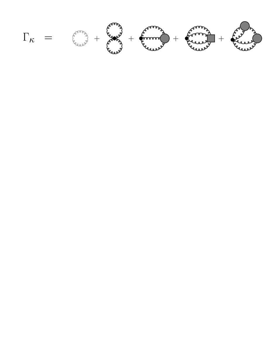
FIG. 2.: Diagrammatic representation of the effective action ${\overline{\Gamma}}_{\kappa}={\overline{\Gamma}}^{(0)}_{\kappa}+\widehat{\overline{\Gamma}}_{\kappa}$, eqs. (64)-(71): the first term is the ‘kinetic’ term, the second term is the tadpole contribution, the third contribution is the 2-gluon loop with exact 3-vertex, the fourth term is the three-loop contribution with exact 4-vertex and the last diagram is the three-loop contribution with two exact 3-vertices. The curly lines represent the exact gluon propagator in the presence of the infrared cut-off $\kappa$, the dots are bare 3-gluon or 4-gluon vertices vertices, while the shaded circles (boxes) are exact 3-gluon and 4-gluon vertices.

E Evolution equation for the average effective action

Following Ref. [3], one can derive an exact evolution equation for the average effective action $\overline{\Gamma}_{\kappa}$ defined by (59), which a type of renormalization group equation which governs the scale-dependence of $\overline{\Gamma}_{\kappa}$ as the infrared cut-off $\kappa$ is varied. Let us introduce the dimensionless evolution variable,

$$t\;\,\equiv\;\,\ln\left(\frac{\kappa}{\Lambda}\right)\;,\;\;\;\;\;\;\;\;\;dt\;\,=\;\,\frac{d\kappa}{\kappa}\;\,=\;\,\frac{1}{2}\;\frac{d\kappa^{2}}{\kappa^{2}}\;.$$ (74)

where $\Lambda$ is some convenient mass scale at which the theory is normalized (Secs. IV and V), and which may be chosen to match a specific physics situation, e.g., the total invariant mass of a high-energy particle collision, or the large momentum transfer in a hard scattering process. Recalling (59), and introducing for abbrevation

$$K[{\cal A},\overline{A},{\cal J}]\;\equiv\;\;\exp\left[\;\frac{}{}i\left(S_{\rm eff}[{\cal A},{\cal J}]+\Re_{\kappa}[{\cal A}]-{\cal J}\circ\overline{A}\right)\right]\,,$$ (75)

one obtains for the derivative of $\Gamma_{\kappa}$, using (18 – 21, 27, 42),

$$\frac{\partial}{\partial t}\,\Gamma_{\kappa}[\overline{A}]\; = \;\frac{\partial}{\partial t}\,W_{\kappa}^{({\cal A})}[{\cal J}]\;\;=\;\;-i\,\frac{\partial}{\partial t}\;\ln\left[\int\,{\cal D}{\cal A}\;K\left[{\cal A},\overline{A},{\cal J}\right]\right]\;\;=\;\;\left.\frac{\int\,{\cal D}{\cal A}\;\frac{1}{2}{\cal A}_{\mu}\,\left(\frac{\partial}{\partial t}{\cal R}_{\kappa}^{\mu\nu}\right)\,{\cal A}_{\nu}\,\;\;K\left[{\cal A},\overline{A},{\cal J}\right]}{\int\,{\cal D}{\cal A}\;\;K\left[{\cal A},\overline{A},{\cal J}\right]}\right|_{{\cal J}=0}$$ (76)

$$= \;\;\frac{1}{2}\;\mbox{Tr}\,\left[\frac{}{}\;\left(\frac{\partial}{\partial t}\,{\cal R}_{\kappa}\right)\;\;\left(\frac{}{}{\cal G}_{\kappa}^{(2)}\;+\;\overline{A}\,\circ\,\overline{A}\right)\right]\;,$$ (78)

while for the derivative of the second term on the right-hand side of (59) one has

$$\frac{\partial}{\partial t}\,\Re_{\kappa}[\overline{A}] = \left.\frac{1}{\int\,{\cal D}{\cal A}\;\;K\left[{\cal A},\overline{A},{\cal J}\right]}\;\;\left(\frac{1}{2}\;\frac{\partial}{\partial t}\,\;{\cal R}_{\kappa}^{\mu\nu}\right)\;\;\left(\frac{}{}\int\,{\cal D}{\cal A}\;{\cal A}_{\mu}\;\;K\left[{\cal A},\overline{A},{\cal J}\right]\;\;\int\,{\cal D}{\cal A}\;{\cal A}_{\nu}\;\;K\left[{\cal A},\overline{A},{\cal J}\right]\right)\;\right|_{{\cal J}=0}$$ (79)

$$= \;\;\frac{1}{2}\;\mbox{Tr}\,\left[\frac{}{}\;\left(\frac{\partial}{\partial t}\,{\cal R}_{\kappa}\right)\;\;\left(\frac{}{}\overline{A}_{\mu}\,\circ\,\overline{A}_{\nu}\right)\right]\;,$$ (81)

where $\mbox{Tr}\left[\ldots\right]$ stands for the trace over all internal indices, as well as an integration over continuous variables. Subtracting (81) from (78), utilizing that ${\cal G}_{k}^{(2)}=(\Gamma_{\kappa}^{(2)})^{-1}=(\overline{\Gamma}_{\kappa}^{(2)}+{\cal R}_{\kappa})^{-1}$, where $\overline{\Gamma}_{\kappa}^{(2)}$ is the second functional derivative of $\overline{\Gamma}_{\kappa}$ with respect to $\overline{A}$, one arrives at the desired evolution equation for the effective average action (59):

$$\frac{\partial}{\partial t}\,\overline{\Gamma}_{\kappa}[\overline{A}] = \;\;\frac{1}{2}\;\mbox{Tr}\,\left[\frac{}{}\left(\frac{\partial}{\partial t}\,{\cal R}_{\kappa}\right)\;\,\left(\overline{\Gamma}_{\kappa}^{(2)}\;+\;{\cal R}_{\kappa}\right)^{-1}\right]\;\;\;\equiv\;\;\;{\cal\gamma}_{\kappa}[\overline{A}]\;.$$ (82)

III The evolution equation for the gluon propagator

Working henceforth in momentum space, we now take practical steps to solve the evolution equation (82) for the gluon propagator. Recall that we defined the exact gluon propagator, respectively its inverse, as (c.f. (44, 45)):

$$\Delta_{\kappa,\,\mu\nu}^{\;\;\;ab}(q) = \;\left({\cal G}_{\kappa}^{(2)}(q,-q)\right)_{\mu\nu}^{ab}\;\;=\;\;\langle\;{\cal A}_{\mu}^{a}(q)\;{\cal A}_{\nu}^{b}(-q)\;\rangle_{\kappa}\;,$$ (83)

$$(\Delta_{\kappa}^{-1})_{\mu\nu}^{ab}(q) = \;\left({\Gamma}_{\kappa}^{(2)}(q,-q)\right)_{\mu\nu}^{ab}\;\;=\;\;\left(\overline{\Gamma}_{\kappa}^{(2)}(q,-q)\right)_{\mu\nu}^{ab}+{\cal R}_{\kappa,\,\mu\nu}^{\;\;\;ab}(q^{2})$$ (84)

Our goal is now to infer from the general evolution equation (82) for the average effective action $\overline{\Gamma}_{\kappa}$ a corresponding evolution equation for $\Delta_{\kappa}^{-1}$, from which we can then determine the properties of the propagator $\Delta_{\kappa}$ itself.

A The general case

We begin by rewriting (82) as

$$\frac{\partial}{\partial t}\,\overline{\Gamma}_{\kappa}[\overline{A}] = \frac{1}{2}\int\frac{d^{4}q}{(2\pi)^{4}}\;\;\left(\frac{\partial}{\partial t}\,{\cal R}_{\kappa}(q^{2})\right)_{\mu\nu}^{ab}\;\,\left(\frac{}{}\left[\overline{\Gamma}_{\kappa}^{(2)}(q,-q)\,+\,{\cal R}_{\kappa}(q^{2})\right]^{-1}\right)_{ab}^{\mu\nu}\;\;\;\equiv\;\;\;{\cal\gamma}_{\kappa}[\overline{A}]\;.$$ (85)

As this is an exact equation, any attempt to solve it in full is certainly out of question, because it would require to solve for an infinite number of the vertex functions $\overline{\Gamma}_{\kappa}^{(n)}$ which contribute to both sides of (85). On the left-hand side, the $\overline{\Gamma}_{\kappa}^{(n)}$ enter through the series representation of $\overline{\Gamma}_{\kappa}[\overline{A}]$,

$$\overline{\Gamma}_{\kappa}[\overline{A}]\;=\;\sum_{n=0}^{\infty}\;\frac{1}{n!}\;\int\frac{d^{4}q_{n}}{(2\pi)^{4}}\ldots\frac{d^{4}q_{1}}{(2\pi)^{4}}\;\left(\overline{\Gamma}_{\kappa}^{(n)}(q_{1},\ldots q_{n})\right)_{\mu_{1}\ldots\mu_{n}}^{a_{1}\ldots a_{n}}\;\overline{A}_{a_{1}}^{\mu_{1}}(q_{1})\ldots\overline{A}_{a_{n}}^{\mu_{n}}(q_{n})\;,$$ (86)

while on the right-hand side of (85), the $\overline{\Gamma}_{\kappa}^{(n)}$ are implicitly encoded in the 2-point function $\overline{\Gamma}_{\kappa}^{(2)}$. However, since we are here interested in the behavior of only the gluon propagator $\Delta_{\kappa}^{\mu\nu}=\langle{\cal A}^{\mu}{\cal A}^{\nu}\rangle_{\kappa}$, we do not need to solve (85) for the average effective action $\overline{\Gamma}_{\kappa}[\overline{A}]$ as a whole, but only for its contributions $\overline{\Gamma}_{\kappa}^{(2)}[\overline{A}]$ which are second order in $\overline{A}$ on the left-hand side of (85), and which are mapped on the corresponding quadratic contributions on the right-hand side, denoted by $\gamma_{\kappa}^{(2)}[\overline{A}]$, being the second order term in the series

$$\gamma_{\kappa}[\overline{A}]\;=\;\sum_{n=0}^{\infty}\;\,\gamma_{\kappa}^{(n)}\;.$$ (87)

That is, instead of (85) for the full $\overline{\Gamma}_{\kappa}$, we aim at the corresponding evolution equation with respect to $t=\ln\kappa$ for the 2-point contributions alone,

$$\;\;\;\;\;\;\;\;\;\;\;\frac{\partial}{\partial t}\,\overline{\Gamma}^{(2)}_{\kappa}\;=\;{\gamma}_{\kappa}^{(2)}\;.$$ (88)

We emphasize that (88) is still an exact equation: no truncations have been imposed on the way from the original evolution equation (85). If we were to know $\gamma_{\kappa}^{(2)}$ exactly, then it would be straightforward to solve for the evolution of $\overline{\Gamma}^{(2)}_{\kappa}$ with $\kappa$. Unfortunately, the function $\gamma_{\kappa}^{(2)}$ on the right-hand side is a tremendously complicated object, because it implicitly contains all sorts of contributions of higher order in the gauge fields, which one would have to determine by solving corresponding equations for $\overline{\Gamma}_{\kappa}^{(3)}$, $\overline{\Gamma}_{\kappa}^{(4)}$, and so forth. Fortunately, the gauge symmetries of QCD allow to relate these higher-order contributions among each other via the Slavnov-Taylor identities, and it is possible, as we shall demonstrate, to obtain a closed expression for $\gamma_{\kappa}^{(2)}$ without explicit knowledge of the higher-order terms, but rather by their implicit inclusion through the constraint equations that follow from first principles .

1 Left-hand side of the evolution equation (88)

Returning to (85), we pick out from the series representation of $\overline{\Gamma}_{\kappa}[\overline{A}]$ in (86) the contribution $\overline{\Gamma}_{\kappa}^{(2)}[\overline{A}]$ that is quadratic in $\overline{A}$, and then consider $\overline{A}=0$,

$$\overline{\Gamma}_{\kappa}^{(2)}\;\equiv\;\overline{\Gamma}_{\kappa}^{(2)}[\overline{A}=0]\;=\;\left.\frac{1}{2}\int\frac{d^{4}q}{(2\pi)^{4}}\;\overline{A}_{a}^{\mu}(q)\;\left(\overline{\Gamma}_{\kappa}^{(2)}(q,-q)\right)_{\mu\nu}^{ab}\;\overline{A}_{b}^{\nu}(-q)\;\right|_{\overline{A}=0}\;.$$ (89)

Now, the two-point function under the integral on the right-hand side is related to the inverse gluon propagator by $(\Delta_{\kappa})^{-1}_{\mu\nu}=\overline{\Gamma}_{\kappa,\,\mu\nu}^{(2)}+{\cal R}_{\kappa,\,\mu\nu}$, since $\overline{\Gamma}_{\kappa,\,\mu\nu}^{(2)}={\Gamma}_{\kappa,\,\mu\nu}^{(2)}-{\cal R}_{\kappa,\,\mu\nu}$ and $\Gamma_{\kappa,\,\mu\nu}^{(2)}=({\cal G}^{(2)}_{\kappa})_{\mu\nu}^{-1}=(\Delta_{\kappa})_{\mu\nu}^{-1}$. We may, therefore, parametrize $\overline{\Gamma}_{\kappa,\,\mu\nu}^{(2)}$ according to the most general tensor decomposition of the inverse propagator $(\Delta_{\kappa})^{-1}_{\mu\nu}$ that is compatible with the constraining Ward identities for the class of axial gauges. This requires two independent scalar functions, $a_{\kappa}(q)$ and $b_{\kappa}(q)$, in which the $q$-dependence can only involve [33] the two invariants $q^{2}/\Lambda^{2}$ and $n^{2}q^{2}/(n\cdot q)^{2}$. Introducing the variable

$$\chi\;\;\equiv\;\;\chi(n,q)\;\;=\;\;\frac{n^{2}\,q^{2}}{(n\cdot q)^{2}}\;,$$ (90)

the dependence of $a_{\kappa}$ and $b_{\kappa}$ on $q$ and $n$ appears as $a_{\kappa}(q)=a_{\kappa}(q^{2},\chi)$, $b_{\kappa}(q)=b_{\kappa}(q^{2},\chi)$. Hence, we can represent $\overline{\Gamma}_{\kappa\,\mu\nu}^{(2)}$ in the following form,

$$\;\left(\overline{\Gamma}_{\kappa}^{(2)}(q,-q)\right)_{\mu\nu}^{ab}\;\;=\;\;\delta^{ab}\left(\frac{}{}a_{\kappa}(q^{2},\chi)\;P_{\mu\nu}(q)\;+\;b_{\kappa}(q^{2},\chi)\;Q_{\mu\nu}(q)\right)\;,$$ (91)

with the orthogonal projection operators

$$P_{\mu\nu}(q) = \;g_{\mu\nu}\;+\;\frac{1}{1-\chi}\,\left[\;\;\chi\,\frac{q_{\mu}q_{\nu}}{q^{2}}\,-\,\frac{n_{\mu}q_{\nu}+q_{\mu}n_{\nu}}{n\cdot q}\,+\,\chi\,\frac{n_{\mu}n_{\nu}}{n^{2}}\right]$$ (92)

$$Q_{\mu\nu}(q) = \;\;-\;\frac{1}{1-\chi}\;\;\left[\;\;\frac{q_{\mu}q_{\nu}}{q^{2}}\,-\,\frac{n_{\mu}q_{\nu}+q_{\mu}n_{\nu}}{n\cdot q}\,+\,\left(\chi\,-\,\frac{(1-\chi)n^{2}}{\xi q^{2}}\right)\,\frac{n_{\mu}n_{\nu}}{n^{2}}\right]\;,$$ (93)

which have been constructed from the available vectors $q_{\mu}$, $n_{\mu}$ and from $g_{\mu}$ in the space $n_{\mu}P^{\mu\nu}=0=n_{\mu}Q^{\mu\nu}$. In the absence of interactions, the bare parameters would be $a_{\kappa}\rightarrow q^{2}+R_{\kappa}$ and $b_{\kappa}\rightarrow q^{2}+R_{\kappa}$. In general, however, the scalar functions $a_{\kappa}$ and $b_{\kappa}$ in (91) embody the full information about the running of $\overline{\Gamma}_{\kappa}^{(2)}$ and, hence, of the gluon propagator which is determined by the inverse of $\overline{\Gamma}_{\kappa}^{(2)}$, as we shall show below.

2 Right-hand side of the evolution equation (88)

Similar as above, we need to extract from ${\gamma}_{\kappa}[\overline{A}]$ in (85) the contribution ${\gamma}_{\kappa}^{(2)}[\overline{A}]$ that is quadratic in $\overline{A}$ and then set $\overline{A}=0$. We first notice that

$$\gamma_{\kappa}\;\equiv\;\gamma_{\kappa}[\overline{A}=0]\;=\;\frac{1}{2}\int\frac{d^{4}q}{(2\pi)^{4}}\frac{d^{4}q^{\prime}}{(2\pi)^{4}}\,\delta^{4}(q+q^{\prime})\;\left(\frac{\partial}{\partial t}\,{\cal R}_{\kappa}(q^{2})\right)_{\mu\nu}^{ab}\;\,\left(\frac{}{}\left[{\Gamma}_{\kappa}^{(2)}(q,q^{\prime})\right]^{-1}\right)_{\mu\nu}^{ab}$$ (94)

where ${\cal R}_{\kappa}(q)$ is the Fourier transform of (32),

$${\cal R}_{\kappa\,,\mu\nu}^{\;\,ab}(q)\;=\;{R}_{\kappa}(q^{2})\;\delta^{ab}\,\left(g_{\mu\nu}\,-\,\frac{q_{\mu}q_{\nu}}{q^{2}}\right)\;=\;{R}_{\kappa}(q^{2})\;\delta^{ab}\,\left(\,P_{\mu\nu}+Q_{\mu\nu}\right)\;.$$ (95)

Next, we decompose $\Gamma_{\kappa}^{(2)}$ in (94) into a kinetic term ($\Pi_{\kappa}^{(0)}$) and an interaction term ($\widehat{\Pi}_{\kappa}$),

$$(\Gamma_{\kappa}^{(2)})_{\mu\nu}^{ab}(q,q^{\prime})\;\;=\;\;\left(\frac{}{}\Pi_{\kappa}^{(0)}\;\;+\;\;\widehat{\Pi}_{\kappa}\,\right)_{\mu\nu}^{ab}(q,q^{\prime})\;.$$ (96)

From the relations (72), we infer

$$\Pi_{\kappa,\,\mu\nu}^{(0)\,ab}(q,q^{\prime}) = \;\;\;\;\;\;\left.\frac{\delta^{2}{\Gamma}_{\kappa}^{(0)}}{\delta\overline{A}_{a}^{\mu}(q)\delta\overline{A}_{b}^{\mu}(q^{\prime})}\right|_{\overline{A}=0}\;=\;\;\;\;2i\;\delta^{4}(q+q^{\prime})\;\,\frac{\delta{\Gamma}_{\kappa}^{(0)}}{\delta\Delta_{\kappa\,ab}^{\;\mu\nu}(q)}$$ (97)

$$\widehat{\Pi}_{\kappa,\,\mu\nu}^{\;\;\,ab}(q,q^{\prime}) = \left.\;\;\;\;\;\;\frac{\delta^{2}\widehat{\Gamma}_{\kappa}}{\delta\overline{A}_{a}^{\mu}(q)\delta\overline{A}_{b}^{\mu}(q^{\prime})}\right|_{\overline{A}=0}\;=\;2i\;\delta^{4}(q+q^{\prime})\;\frac{\delta\widehat{\Gamma}_{\kappa}}{\delta\Delta_{\kappa\,ab}^{\;\mu\nu}(q)}\;.$$ (98)

Applying these to the formulae (63 – 71), after Fourier transformation to momentum space, we obtain for the kinetic term

$$\Pi^{(0)\;ab}_{\kappa,\,\mu\nu}(q,-q) = \;\;\;\;\delta_{ab}\,\left(q^{2}+R_{\kappa}(q^{2})\right)\;\left(\;g_{\mu\nu}\,-\,\frac{q_{\mu}q_{\nu}}{q^{2}}\,+\;\frac{1}{\xi}\,\frac{n_{\mu}n_{\nu}}{q^{2}}\right)\;,$$ (99)

while the interaction term gives

$$\widehat{\Pi}^{\;\;ab}_{\kappa,\,\mu\nu}(q,-q) = \;\,\,\frac{g^{2}}{2}\;\int\frac{d^{4}k}{(2\pi)^{4}}\;\;W_{\;\;\mu\nu\lambda\sigma}^{(0),abcd}(q,k,-k,-q)\;{\Delta}_{\kappa}^{\lambda\sigma\,,cd}(k)\;$$ (105)

$$-\,\frac{i\,g^{2}}{2}\;\int\frac{d^{4}k}{(2\pi)^{4}}\;\;V_{\;\;\mu\lambda\sigma}^{(0),acd}(q,-k,-k^{\prime})\;\;{\Delta}_{\kappa}^{\lambda\lambda^{\prime},\,cc^{\prime}}(k)\;{\Delta}_{\kappa}^{\sigma\sigma^{\prime},\,dd^{\prime}}(k^{\prime})\;{\cal V}_{\sigma^{\prime}\lambda^{\prime}\nu}^{d^{\prime}c^{\prime}b}(k^{\prime},k,-q)$$

$$+\;\frac{g^{4}}{6}\;\int\frac{d^{4}k}{(2\pi)^{4}}\frac{d^{4}p}{(2\pi)^{4}}\;\;{W}_{\;\;\mu\lambda\sigma\tau}^{(0),acde}(q,-k,-k^{\prime},-p)\;\;{\Delta}_{\kappa}^{\lambda\lambda^{\prime},\,cc^{\prime}}(k)\;{\Delta}_{\kappa}^{\sigma\sigma^{\prime},\,dd^{\prime}}(k^{\prime})\;$$

$$\;\;\;\;\;\;\;\;\;\;\;\;\;\;\;\;\;\;\;\;\;\;\;\;\;\;\;\;\;\;\;\;\;\;\;\;\;\;\;\;\;\;\;\;\;\;\;\;\;\;\;\;\;\;\;\;\times\;{\Delta}_{\kappa}^{\tau\tau^{\prime},\,ee^{\prime}}(p)\;{\cal W}_{\tau^{\prime}\sigma^{\prime}\lambda^{\prime}\nu}^{e^{\prime}d^{\prime}c^{\prime}b}(k,k^{\prime},p,-q)$$

$$+\;\frac{g^{4}}{24}\;\int\frac{d^{4}k}{(2\pi)^{4}}\frac{d^{4}p}{(2\pi)^{4}}\;\;W_{\;\;\mu\lambda\sigma\tau}^{(0),acde}(q,-k,-k^{\prime},-p^{\prime})\;\;{\Delta}_{\kappa}^{\sigma\rho^{\prime},\,df^{\prime}}(k)\;{\Delta}_{\kappa}^{\tau\rho^{\prime\prime},\,ef^{\prime\prime}}(k^{\prime})\;$$

$$\;\;\;\;\;\;\;\;\;\;\;\;\;\;\;\;\;\;\;\;\;\;\;\;\;\;\;\;\;\;\;\times\;{\cal V}_{\rho^{\prime\prime}\rho^{\prime}\rho}^{f^{\prime\prime}f^{\prime}f}(k,k^{\prime},-p)\;\;{\Delta}_{\kappa}^{\rho\lambda^{\prime},\,fc^{\prime}}(p)\;{\Delta}_{\kappa}^{\lambda\sigma^{\prime},\,cd^{\prime}}(p^{\prime})\;\;\;{\cal V}_{\lambda^{\prime}\sigma^{\prime}}^{c^{\prime}d^{\prime}}(p,p^{\prime},-q)\;,$$

with $k^{\prime}=q-k$ in the second term, $k^{\prime}=q-k-p$ in the third term, and $k^{\prime}=q-k-p^{\prime},\;p^{\prime}=q-p$ in the last term. Fig. 3 depicts diagramatically the inverse propagator $(\Gamma_{\kappa}^{(2)})_{\mu\nu}$, eq. (96), in terms of the contributions $\Pi_{\kappa}^{(0)}$, eq. (65), and $\widehat{\Pi}_{\kappa}$, eq. (71).

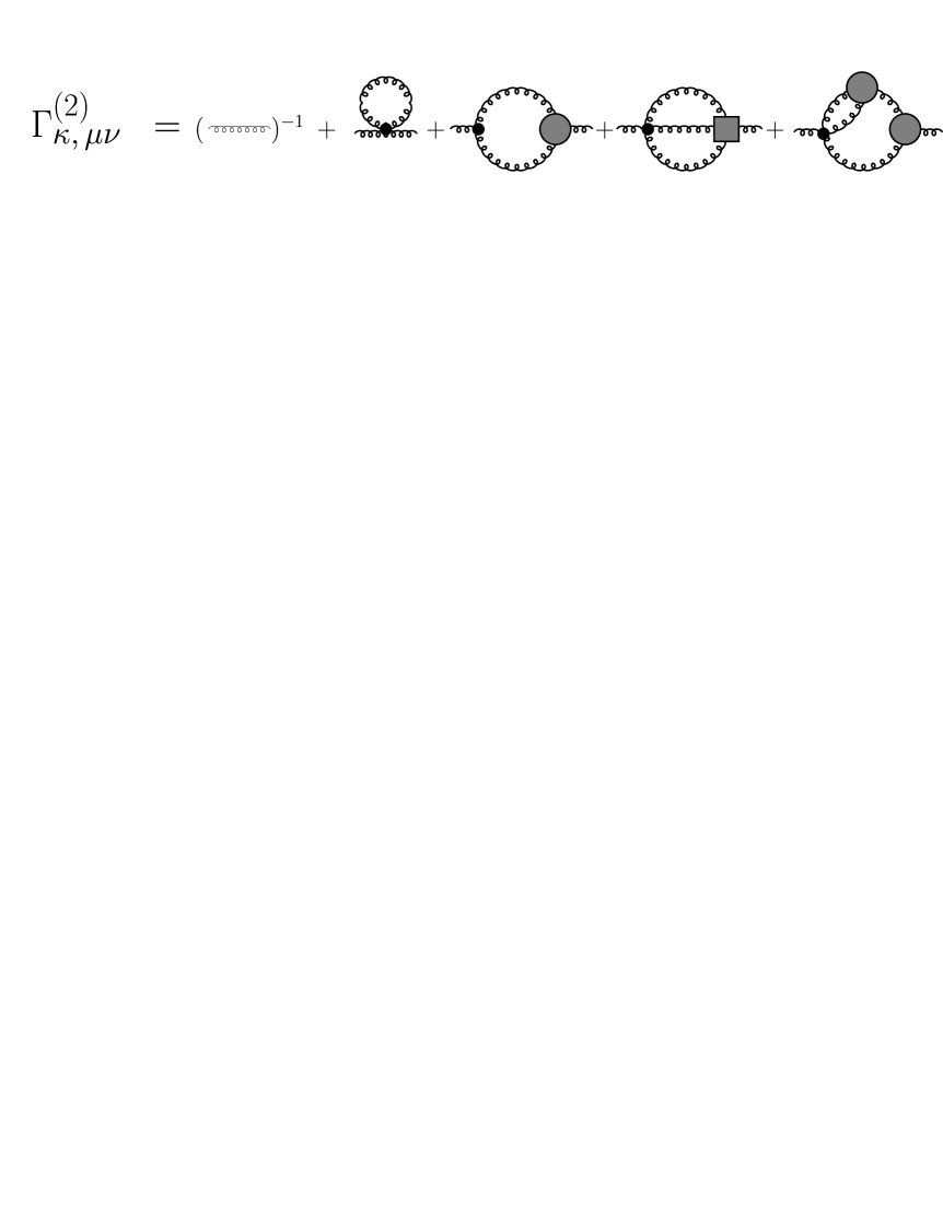
FIG. 3.: Diagrammatic representation of the inverse propagator $(\Gamma_{\kappa}^{(2)})_{\mu\nu}=(\Pi_{\kappa}^{(0)}+\widehat{\Pi}_{\kappa})_{\mu\nu}$, eqs. (96)-(105). The first term is the contribution from the ‘kinetic part’ $\Pi^{(0)}_{\kappa}$, while the remaining terms arise from the ‘interaction part’ $\widehat{\Pi}_{\kappa}$. The curly lines represent the exact gluon propagator in the presence of the infrared cut-off $\kappa$, the dots are bare 3-gluon or 4-gluon vertices vertices, while the shaded circles (boxes) are exact 3-gluon and 4-gluon vertices.

Now let us define a partial derivative $\partial^{\ast}_{t}$ that acts only on the $t=\ln\kappa$ dependence of $\Pi^{(0)}_{\kappa}$, but not on $\widehat{\Pi}_{\kappa}$,

$$\partial^{\ast}_{t}\,\Gamma_{\kappa}^{(2)}\;\;:=\;\;\partial^{\ast}_{t}\,\left(\Pi^{(0)}_{\kappa}+\widehat{\Pi}_{\kappa}\right)\;\;=\;\;\partial^{\ast}_{t}\,\Pi^{(0)}_{\kappa}\;\;=\;\;\frac{\partial}{\partial t}\Pi^{(0)}_{\kappa}\;,$$ (106)

so that we may write the right-hand side of eq. (85) in a form that is reminescent of the derivative of a one-loop expression, but which is exact,

$${\gamma}_{\kappa}\;\;=\;\;\frac{1}{2}\int\frac{d^{4}q}{(2\pi)^{4}}\;\;\partial^{\ast}_{t}\,\left[\frac{}{}\ln\left.{\Gamma}_{\kappa}^{(2)}\right._{\mu\,a}^{\mu\,a}(q,-q)\right]\;\;=\;\;\frac{1}{2}\,\mbox{Tr}\left[\frac{\partial^{\ast}}{\partial t}\ln\left.{\Gamma}_{\kappa}^{(2)}\right.\right]\;.$$ (107)

From this representation of $\gamma_{\kappa}$ we extract now the contribution which corresponds to terms quadratic in the gluon fields, and therefore is relevant for the evolution of the gluon propagator: We utilize

$$\mbox{Tr}\,[\;\partial_{t}^{\ast}\ln\Gamma_{\kappa}^{(2)}\;]\;=\;\mbox{Tr}\,[\;\ln\Pi_{0}\;]\;+\;\mbox{Tr}\,[\;\partial_{t}^{\ast}(\;\widehat{\Pi}_{\kappa}\;\Pi_{\kappa}^{(0)\;-1})]\;-\;\frac{1}{2}\mbox{Tr}\,[\;\partial_{t}^{\ast}(\;\widehat{\Pi}_{\kappa}\;\Pi_{\kappa}^{(0)\;-1}\;\widehat{\Pi}_{\kappa}\;\Pi_{\kappa}^{(0)\;-1})\;]\;+\;\ldots\;,$$ (108)

where the dots refer to higher-order terms which are cubic and higher in the gluon fields and therefore contribute only to the 3-point, 4-point functions, etc., but not to the gluon propagator or its inverse. Now, the first term in (108) amounts to an irrelevant constant which may be dropped in view of (99), so that we finally arrive at

$${\gamma}_{\kappa}^{(2)} = \;\;\;\,\frac{1}{2}\,\int\frac{d^{4}q}{(2\pi)^{4}}\;\;\partial^{\ast}_{t}\left[\frac{}{}\widehat{\Pi}_{\kappa,\,\mu\nu}^{\;\;\;ab}(q,-q)\;\,(\Pi_{\kappa}^{-1})_{ba}^{\nu\mu}(-q,q)\right]$$ (110)

$$-\;\frac{1}{4}\,\int\frac{d^{4}q}{(2\pi)^{4}}\,\frac{d^{4}p}{(2\pi)^{4}}\;\;\partial^{\ast}_{t}\left[\frac{}{}\widehat{\Pi}_{\kappa,\,\mu\lambda}^{\;\;\;ac}(q,-p)\,\;(\Pi_{\kappa}^{-1})_{cd}^{\lambda\sigma}(-p,p)\;\,\widehat{\Pi}_{\kappa,\,\sigma\tau}^{\;\;\;de}(p,-q)\,\;(\Pi_{\kappa}^{-1})_{ea}^{\sigma\mu}(-q,q)\right]\;.$$

3 The master equations for the gluon propagator

Now we have collected all the ingredients for the evolution equation (88): $\overline{\Gamma}_{\kappa}^{(2)}$ appearing on the left-hand side, is given by (89 – 92), and ${\gamma}_{\kappa}^{(2)}$ on the right-hand side, is determined by (110) together with (99) and (105). In order to infer from this evolution equation two independent, coupled scalar equations for the two unknown functions $a_{\kappa}$ and $b_{\kappa}$, we project (88) with $P_{\mu\nu}$ and $Q_{\mu\nu}$, given by (93) and (92), respectively. Using $P_{\mu\lambda}P^{\lambda}_{\nu}=P_{\mu\nu}$, $Q_{\mu\lambda}Q^{\lambda}_{\nu}=Q_{\mu\nu}$, and $P_{\mu\lambda}Q^{\lambda}_{\nu}=0$, as well as $n^{\mu}(\Pi_{\kappa}^{(0)\;-1})_{\mu\nu}=0$, $q^{\mu}(\widehat{\Pi}_{\kappa})_{\mu\nu}=0$, we obtain after some algebra,

$$\frac{\partial}{\partial t}\,a_{\kappa}(q^{2},\chi) = \;\frac{1}{2}\;\left(\;g_{\mu\nu}\;+\;\frac{\chi}{1-\chi}\frac{n_{\mu}n_{\nu}}{n^{2}}\;\right)\;\;\frac{\partial}{\partial t}\;\widehat{\Pi}_{\kappa}^{\mu\nu}(q,-q)$$ (111)

$$\frac{\partial}{\partial t}\,b_{\kappa}(q^{2},\chi) = \;\;-\;\frac{\chi}{1-\chi}\;\frac{n_{\mu}n_{\nu}}{n^{2}}\;\;\frac{\partial}{\partial t}\;\widehat{\Pi}_{\kappa}^{\mu\nu}(q,-q)\;.$$ (112)

We remind the reader of the complexity of these equations, which are equivalent to (88), and hence our comments after (88) apply also here. The key problem becomes clear in view of (105), which shows that $\widehat{\Pi}_{\kappa}$ contains not only the exact propagator $\Delta_{\kappa}$, but also the exact 3-gluon and 4-gluon vertex functions ${\cal V}$, respectively ${\cal W}$. In principle, one would therefore have to solve even more complicated equations for ${\cal V}$ and ${\cal W}$, and then plug the solutions into $\widehat{\Pi}_{\kappa}$ of (105). Then (112) and (111) would contain on the right-hand sides only the unknown $\Delta_{\kappa}$, the solution of which we are after. However, as we show in the next subsections, it is possible to get rid of the explicit dependence on ${\cal V}$ and ${\cal W}$ by (i) eliminating the 4-gluon vertices and (ii) expressing the 3-gluon vertices through the propagator $\Delta_{\kappa}$ alone. Then we can evaluate $\widehat{\Pi}_{\kappa}$, (112) and (111) serve to determine the functions $a_{\kappa}$ and $b_{\kappa}$ which, in turn, would give a unique solution to the exact gluon propagator from (96),

$$\Delta_{\kappa,\,\mu\nu}^{\;\;ab}(q)\;=\;\left({\Gamma}_{\kappa}^{(2)\;-1}\right)_{\mu\nu}^{ab}(q,-q)\;\;=\;\;\left(\left[\Pi_{\kappa}^{(0)}\;+\widehat{\Pi}_{\kappa}\right]^{-1}\right)_{\mu\nu}^{ab}$$ (113)

Decomposing the propagator analogous to (91),

$$\Delta_{\kappa,\,\mu\nu}^{\;\;ab}(q)\;=\;\delta^{ab}\left(\frac{}{}A_{\kappa}(q^{2},\chi)\;S_{\mu\nu}(q)\;+\;B_{\kappa}(q^{2},\chi)\;T_{\mu\nu}(q)\right)\;,$$ (114)

with the projectors

$$S_{\mu\nu}(q) = \;g_{\mu\nu}\;+\;\frac{1}{1-\chi}\,\left[\;\chi\;\left(1+\xi q^{2}\right)\,\frac{q_{\mu}q_{\nu}}{q^{2}}\,-\,\frac{n_{\mu}q_{\nu}+q_{\mu}n_{\nu}}{n\cdot q}\,+\,\chi\,\frac{n_{\mu}n_{\nu}}{n^{2}}\right]$$ (115)

$$T_{\mu\nu}(q) = \;\;-\;\frac{1}{1-\chi}\;\;\left[\;\chi\;\left(1+\xi q^{2}\right)\,\frac{q_{\mu}q_{\nu}}{q^{2}}\,-\,\frac{n_{\mu}q_{\nu}+q_{\mu}n_{\nu}}{n\cdot q}\,+\,\frac{n_{\mu}n_{\nu}}{n^{2}}\right]\;,$$ (116)

and inverting $\Pi_{\kappa}^{(0)}+\widehat{\Pi}_{\kappa}$ on the right-hand side of (113), one finds (c.f. Appendix D) that the functions $A_{\kappa}$ and $B_{\kappa}$ are related to $a_{\kappa}$ and $b_{\kappa}$ by

$$A_{\kappa}(q^{2},\chi)\;=\;\frac{1}{a_{\kappa}(q^{2},\chi)}\;,\;\;\;\;\;\;\;\;\;\;\;\;\;\;\;\;B_{\kappa}(q^{2},\chi)\;=\;\frac{\chi}{b_{\kappa}(q^{2},\chi)}\;.$$ (117)

In the limit of vanishing coupling $g\rightarrow 0$, we have $a_{\kappa}\rightarrow q^{2}+R_{\kappa}$ and $b_{\kappa}\rightarrow q^{2}+R_{\kappa}$, so that the bare propagator $\Delta_{\kappa}^{(0)}$, respectively its inverse $\Pi_{\kappa}^{(0)}$ are,

$$\Delta_{\kappa,\;\mu\nu}^{(0)}(q)\; = \;\frac{S_{\mu\nu}\,+\,\chi\,T_{\mu\nu}}{q^{2}+R_{\kappa}(q^{2})}$$ (118)

$$= \;\frac{1}{q^{2}+R_{\kappa}(q^{2})}\;\;\left[\;g_{\mu\nu}\,-\,\frac{n_{\mu}q_{\nu}+q_{\mu}n_{\nu}}{n\cdot q}\,+\,(n^{2}+\xi q^{2})\,\frac{q_{\mu}q_{\nu}}{(n\cdot q)^{2}}\right]$$ (119)

$$\Pi_{\kappa,\;\mu\nu}^{(0)}(q,-q)\; = \;\left(q^{2}+R_{\kappa}(q^{2})\right)\;\,\left(\,P_{\mu\nu}\,+\,Q_{\mu\nu}\,\right)$$ (121)

$$= \;\left(q^{2}+R_{\kappa}(q^{2})\right)\;\;\left[\;g_{\mu\nu}\,-\,\frac{q_{\mu}q_{\nu}}{q^{2}}\,+\,\left(n^{2}q^{2}+\frac{1}{\xi}\right)\frac{n_{\mu}n_{\nu}}{(n\cdot q)^{2}}\right]\;,$$ (122)

and, since $\Delta_{\kappa}^{(0)}=\left(\Pi_{\kappa}^{(0)}\right)^{-1}$, the following inversion property holds: $\Delta_{\kappa,\;\mu\lambda}\;(\,\Pi^{(0)}_{\kappa}+\widehat{\Pi}_{\kappa}\,)^{\lambda}_{\;\;\;\nu}=g_{\mu\nu}$.

B The case $\chi\;\rightarrow\;0$

The system of evolution equations (111) and (112) for the functions $a_{\kappa}$, $b_{\kappa}$, and hence for $A_{\kappa}$, $B_{\kappa}$, is still immensely difficult to solve, because, as is evident from (105), the self-energy tensor $\widehat{\Pi}_{\kappa}$ contains products of exact propagators $\Delta_{\kappa}$ (the solution of which we do not know yet) with the exact 3-gluon and 4-gluon vertex functions $\widehat{V}$ and $\widehat{W}$ (which are themselves unknown combinations of propagators). However, we can make substantial progress, if we can eliminate the explicit $\chi$-dependence, by considering $\chi=n^{2}q^{2}/(n\cdot q)^{2}=0$: There are two possibilities to achieve this condition: (i) choosing $n^{2}\rightarrow 0$, or (ii) considering $q^{2}/(n\cdot q)^{2}\rightarrow 0$. The first possibility corresponds to choosing, among all the axial gauges with arbitrary $n^{2}$, the light-cone gauge with $n^{2}=0$. The second possibility, $q^{2}/(n\cdot q)^{2}\rightarrow 0$, holds for any $n^{2}$, and corresponds to the quasi-real limit, by which we mean the kinematic regime in which the gluon energy $q_{0}$ is large as compared to the virtual mass $\sqrt{q^{2}}$ so that the gluons are practically on-shell. Specifically, we require for the gluon four-momentum $q_{\mu}=\left(q_{0},{\bf q}_{\perp},q_{z}\right)$ that

$$q_{0}^{2}\;\;\approx\;\;q_{z}^{2}\;\;\gg\;\;q^{2}_{\perp}\;\;\gg\;q^{2}\;.$$ (123)

This situation is typical for high-energy particle collisions with (gluon) jet production, for example, hadronic collisions with center-of-mass energy $E_{\rm cm}\,\lower 3.0pt\hbox{$\buildrel>\over{\sim}$}\,100$ GeV, where the gluon (and quark) fluctuations in the colliding hadrons have highly boosted longitudinal momentum along the beam axis, and comparably very small transverse momentum. Bearing this physics picture in mind, it is then suggestive to choose the vector $n_{\mu}$ along the preferred longitudinal $z$-direction that is dictated by the collision geometry, i.e., to choose $n_{\mu}$ in the $t$-$z$ plane, parametrized as

$$n_{\mu}\;=\;\left(u+v,{\bf 0}_{\perp},u-v\right)\;\;\;\;\;\;\;\;\;\;\;n^{2}\;=\;4\,u\,v\;.$$ (124)

The two assertions (123) and (124) imply

$$n\cdot q\;\approx\;2\,v\,q_{0}\;\;\;\;\;\;\;\;\mbox{and}\;\;\;\;\;\;\;\;\;\frac{q^{2}}{(n\cdot q)^{2}}\;\simeq\;0\;.$$ (125)

Consequently, from (90) and (117), we have for $q^{2}/(n\cdot q)^{2}\rightarrow 0$ or $n^{2}\rightarrow 0$ (assuming the functions $a_{\kappa}$ and $b_{\kappa}$ are finite for all $q$),

$$\chi\;\;\longrightarrow\;\;0\;,\;\;\;\;\;\;\;\;\;\;\;\;B_{\kappa}=\frac{\chi}{b_{\kappa}}\;\;\longrightarrow\;\;0\;,$$ (126)

so that we are left with only one unknown function $A_{\kappa}=1/a_{\kappa}$. We find that in this limit (111) and (112) coincide, since

$$g_{\mu\nu}\widehat{\Pi}^{\mu\nu}\;\;=\;\;\widehat{\Pi}_{\mu}^{\;\,\mu}\;\;=\;\;-\;3\;\frac{\chi}{1-\chi}\;\frac{n_{\mu}n_{\nu}}{n^{2}}\;\widehat{\Pi}^{\mu\nu}\;,$$ (127)

and therefore only the tensor structure $n_{\mu}n_{\nu}\widehat{\Pi}^{\mu\nu}$ appears in both equations. Using (127) together with the definition of $\chi$, eq. (90), and the expression (105) for $\widehat{\Pi}$, we obtain the master equation for $a_{\kappa}$ in the limit (126),

$$\frac{\partial}{\partial t}\,b_{\kappa}(q^{2},\chi)\; = \;-\,\frac{\chi}{1-\chi}\;\,\frac{n_{\mu}n_{\nu}}{n^{2}}\;\left(\frac{\partial}{\partial t}\;\widehat{\Pi}_{\kappa}^{\mu\nu}(q,-q)\right)$$ (128)

$$\;.\; = \;-\,\left(\frac{q^{2}}{(n\cdot q)^{2}-n^{2}q^{2}}\right)\;\;\left\{\frac{}{}\;\frac{1}{2}g^{2}\;\int\frac{d^{4}k}{(2\pi)^{4}}\;n^{2}\;\left(\frac{\partial}{\partial t}\Delta_{\kappa}^{\lambda\lambda}(k)\right)\right.$$ (129)

$$\;\;\;\;\;\;\;\;\;\;\;\left.\frac{}{}+\;\frac{i}{2}g^{2}\;\int\frac{d^{4}k}{(2\pi)^{4}}\;n\cdot(k-k^{\prime})\;n^{\nu}\;\left(\frac{}{}\frac{\partial}{\partial t}\left[\Delta_{\kappa}^{\lambda\sigma}(k)\;\Delta_{\kappa,\,\lambda}^{\;\;\;\;\,\sigma^{\prime}}(k^{\prime})\;{\cal V}_{\sigma\sigma^{\prime}\nu}(k^{\prime},k,-q)\right]\right)\,\right\}\;,$$ (130)

where $k^{\prime}=q-k$, and we have utilized the form of the bare 3-gluon vertex $V^{(0)}$, as given by (B37). Notice that (129) contains only the tadpole contribution and the 3-gluon vertex contribution, as diagramatically represented in Fig. 4: all the other 4-gluon terms that are present in $\widehat{\Pi}_{\mu\nu}$ of (105) vanish identically upon contraction with $n_{\mu}$ and $n_{\nu}$, because $\Delta_{\kappa}$ is orthogonal to $n$, which is a direct consequence of the orthogonality of $\widehat{\Pi}$ with respect to $q$ due to current conservation (both properties hold, of course, also for the bare functions $\Delta_{\kappa}^{(0)}$ and $\Pi_{\kappa}^{(0)}$),

$$n^{\mu}\,\Delta_{\kappa,\;\mu\nu}\;\;=\;\;0\;\;=\;\;\Delta_{\kappa,\;\mu\nu}\;n^{\nu}\;\;\;\;\;\;\;\;\;\;\;\;\;\;\;\;\;\;\;\;\;q^{\mu}\,\widehat{\Pi}_{\kappa,\;\mu\nu}\;=\;0\;=\;\widehat{\Pi}_{\kappa,\;\mu\nu}\;q^{\nu}\;.$$ (131)

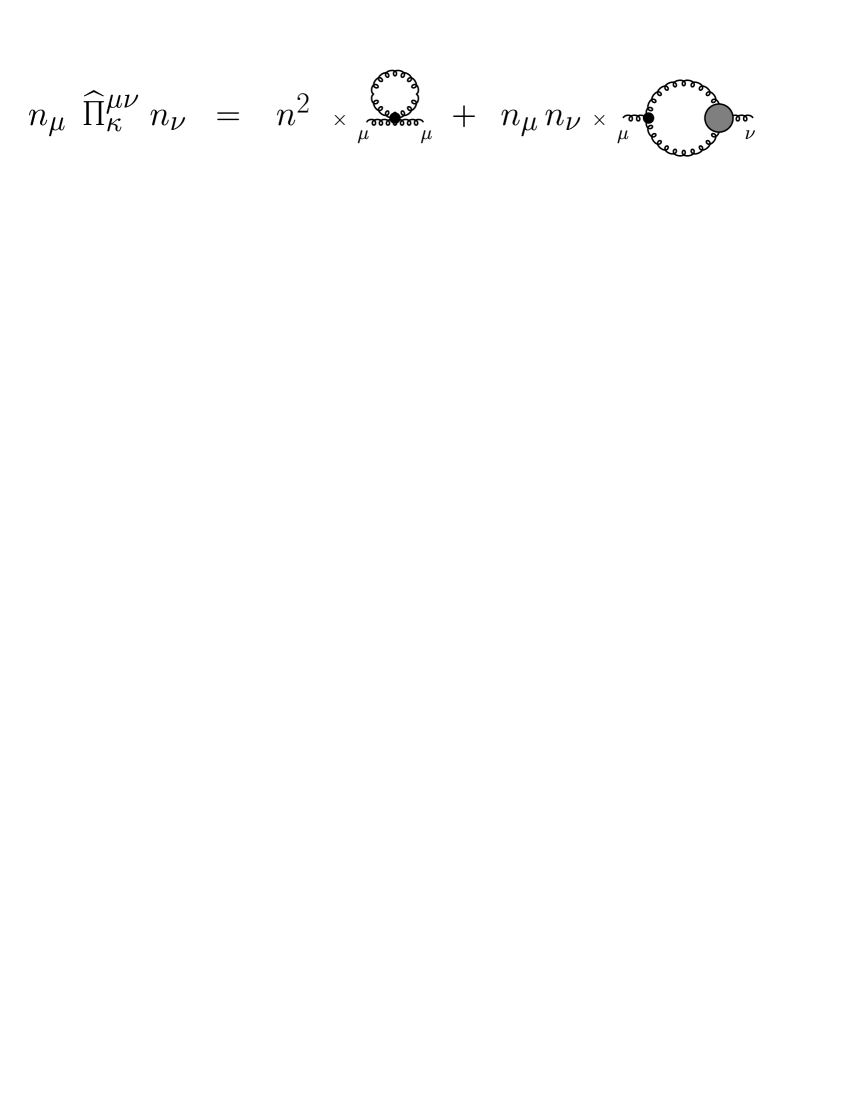
FIG. 4.: Diagrammatics of the contraction $n_{\mu}\widehat{\Pi}_{\kappa}^{\mu\nu}n_{\nu}$: Only the tadpole contribution (proportional to $n^{2}$) and the 3-gluon vertex contribution (proportional to $n_{\mu}n_{\nu}$) survive. All the terms drop out upon contraction with $n_{\mu}$ and $n_{\nu}$,

The initial conditions for the evolution equation (129) are dictated by asymptotic freedom in the ultraviolet limit as $q\rightarrow\infty$, or more precisely, $q^{2}\rightarrow\Lambda^{2}$ with the normalization scale $\Lambda^{2}/\kappa^{2}\rightarrow\infty$ [cf. (74)]:

$$a_{\kappa}(q^{2},\chi)\;\;\stackrel{{\scriptstyle q^{2}\rightarrow\Lambda^{2}}}{{\longrightarrow}}\;\;q^{2}\;,$$ (132)

which implies that the gluon propagator becomes the bare propagator at the renormalization point,

$$\Delta_{\kappa}(q)\;\stackrel{{\scriptstyle q^{2}\rightarrow\Lambda^{2}}}{{\longrightarrow}}\;\;\Delta^{(0)}_{\kappa}(q)\;.$$ (133)

As we move away from the asymptotic normalization scale $\Lambda$, the full gluon propagator propagator (114) remains proportional to its bare counterpart, modulo the function $A_{\kappa}=1/a_{\kappa}$, which encodes all effects of including softer and softer gluon fluctuations in the evolution equation (129),

$$\Delta_{\kappa,\;\mu\nu}(q)\;\;=\;\;\frac{1}{a_{\kappa}(q^{2},\chi)}\;\;S^{\prime}_{\mu\nu}(q)\;\;=\;\;\left(\frac{q^{2}+R_{\kappa}(q^{2})}{b_{\kappa}(q^{2},\chi)}\right)\;\;\Delta^{(0)}_{\kappa,\;\mu\nu}(q)\;,$$ (134)

with $S^{\prime}_{\mu\nu}$ given by (115) at the value $\chi=0$, i.e.,

$$S^{\prime}_{\mu\nu}(q)\;\;=\;\;g_{\mu\nu}\,-\,\frac{n_{\mu}q_{\nu}+q_{\mu}n_{\nu}}{n\cdot q}\;.$$ (135)

Hence, the bare propagator and its inverse (taking now and henceforth $\xi\rightarrow 0$) reads

$$\Delta_{\kappa,\;\mu\nu}^{(0)}(q)\; = \;\frac{1}{q^{2}+R_{\kappa}(q^{2})}\;\left[\;g_{\mu\nu}\,-\,\frac{n_{\mu}q_{\nu}+q_{\mu}n_{\nu}}{n\cdot q}\right]$$ (136)

$$\Pi_{\kappa,\;\mu\nu}^{(0)}(q,-q)\; = \;\left(q^{2}+R_{\kappa}(q^{2})\right)\;\left[\;g_{\mu\nu}\,-\,\frac{q_{\mu}q_{\nu}}{q^{2}}\right]\;,$$ (137)

and the inversion property, noted after eq. (122), is modified for $\xi\rightarrow 0$:   $\Delta_{\kappa,\;\mu\lambda}\;(\,\Pi^{(0)}_{\kappa}+\widehat{\Pi}_{\kappa}\,)^{\lambda}_{\;\;\;\nu}=g_{\mu\nu}\,-\,n_{\mu}q_{\nu}/(n\cdot q)$.

C Remarks

Let us summarize the conceptual steps of the preceding subsections. From the general form of the evolution equation (88) for the quadratic (in the average gauge field) contributions of the average effective action, we inferred a coupled set of equations (111) and (112) that determine the exact form of the gluon propagator via (114) and (117) in terms of the scalar functions $a_{\kappa}$ and $b_{\kappa}$. In the case of $\chi=n^{2}q^{2}/(n\cdot q)^{2}$, we could eliminate the dependence on the function $b_{\kappa}$, and arrived at the master equation (129) for $a_{\kappa}$ alone, the solution of which determines the full gluon propagator by simply mutiplying the bare propagator with the single function $a_{\kappa}$. The presumption $\chi\rightarrow 0$ can be achieved either by letting $n^{2}\rightarrow 0$, or by considering $q^{2}/(n\cdot q)^{2}\rightarrow 0$. The former possibility corresponds to going over to the light-cone gauge, while the latter possibility is fulfilled in the kinematic regime (123) of “quasireal” gluons. In either case, we have the condition (126), under which the master equation (129) is an exact equation in the sense that it contains the full non-perturbative evolution associated with the function $a_{\kappa}$ in general axial gauges specified by the vector $n_{\mu}$ and the gauge parameter $\xi$.

IV Solution for the gluon propagator in the light-cone gauge

Recall that (129) holds for the class of axial gauges (14) in general, viz. for any choice of $n_{\mu}$ with finite $n^{2}$ and arbitrary gauge parameter $\xi$. For $n^{2}\neq 0$, the expression on the right-hand side of this equation is then still very difficult to integrate, as has been discussed, e.g., in Ref. [19] for the case , $n_{\mu}=(1,0,0,0)$ $n^{2}=1$, and $\xi=0$. On the other hand, for $n^{2}=0$, which we will consider in the following, the right-hand side of (129) simplifies considerably, so that an exact (numerical) integration is straightforward. Moreover, we will show that it is even possible to integrate eq. (129) in closed form by utilizing the methods of Ref. [23], with the result being expressable in terms of elementary functions.

A Evolution of the renormalization function ${\cal Z}_{\kappa}$ for $n^{2}=0$

The light-cone gauge can be specified by choosing, in the parametrization (124), the constant vector $n_{\mu}$, such that it is directed along the forward light-cone in the $t-z$ plane. Setting in (124) $u=0$ and $v=1$, we have

$$n_{\mu}\;=\;\left(1,{\bf 0}_{\perp},-1\right)\;\;\;\;\;\;\;\;\;\;\;n^{2}\;=\;0\;.$$ (138)

It follows then that $\chi=0$, and if we introduce instead of $a_{\kappa}$ the dimensionless renormalization function

$${\cal Z}_{\kappa}(q^{2})\;\equiv\;\frac{q^{2}}{a_{\kappa}(q^{2},0)}\;,$$ (139)

with initial condition (132) at the normalization scale $\Lambda^{2}\gg\kappa^{2}$ in the ultraviolet:

$${\cal Z}_{\kappa}(q^{2})\;\;\stackrel{{\scriptstyle q^{2}\rightarrow\Lambda^{2}}}{{\longrightarrow}}\;\;\;1\;,$$ (140)

then we may rewrite the evolution equation (129) as

$$\frac{\partial}{\partial t}\,\frac{1}{{\cal Z}_{\kappa}(q^{2})}\; = \;\frac{\partial}{\partial t}\,\frac{a_{\kappa}(q^{2},0)}{q^{2}}$$ (141)

$$= \;-\,\frac{n_{\mu}n_{\nu}}{(n\cdot q)^{2}}\;\;\left(\frac{\partial}{\partial t}\;\widehat{\Pi}_{\kappa}^{\mu\nu}(q,-q)\right)$$ (142)

$$= \;-\,\frac{i}{2}\;g^{2}\;\int\frac{d^{4}k}{(2\pi)^{4}}\;\frac{n\cdot(k-k^{\prime})}{(n\cdot q)^{2}}\;n^{\nu}\;\left(\frac{}{}\frac{\partial}{\partial t}\left[\Delta_{\kappa}^{\lambda\sigma}(k)\;\Delta_{\kappa,\,\lambda}^{\;\;\;\;\,\sigma^{\prime}}(k^{\prime})\;{\cal V}_{\sigma\sigma^{\prime}\nu}(k^{\prime},k,-q)\right]\right)\;,$$ (143)

in which now only the 3-gluon contribution with the exact vertex function ${\cal V}$ and exact propagators $\Delta_{\kappa}$ is present, while the tadpole contribution, i.e., the first term on the right-hand side of (129), vanishes since it is proportional to $n^{2}$. The solution of (143) then determines the full gluon propagator in terms of ${\cal Z}_{\kappa}$, so that we have instead of (134),

$$\Delta_{\kappa,\;\mu\nu}(q)\;\;=\;\;{\cal Z}_{\kappa}(q^{2})\;\;\Delta^{(0)}_{\kappa,\;\mu\nu}(q)\;,$$ (144)

with the bare propagator $\Delta_{\kappa}^{(0)}$ given by (136).

B The spectral representation of propagator and vertex function

The evolution equation (143) still contains the unknown exact 3-gluon vertex function ${\cal V}$, which, as one would expect, would have to be determined first, by solving a corresponding evolution equation for ${\cal V}$, itself involving higher-order vertex functions. Luckily, the gauge symmetry properties of QCD imply the Slavnov-Taylor identities, which are the Ward identities of QCD relating the vertex functions to the propagator. In general these relations are non-trivial, however, in the class of axial gauges, the Slavnov-Taylor identities have a simple form. For example, the 3-gluon vertex function ${\cal V}$ can be expressed in terms of the propagator $\Delta_{\kappa}$ as

$$q_{\lambda}\,\;{\cal V}_{\lambda\sigma\tau}(q,k,k^{\prime})\;\;\Delta_{\kappa}^{\sigma\mu}(k)\;\;\Delta_{\kappa}^{\tau\nu}(k^{\prime})\;\;=\;\;\Delta_{\kappa}^{\mu\nu}(k^{\prime})\;\;-\;\;\Delta_{\kappa}^{\mu\nu}(k)\;.$$ (145)

where $(k^{\prime}=q-k)$. This Slavnov-Taylor identity suggests the following strategy: (i) construct an ansatz for ${\cal V}$, in terms of $\Delta_{\kappa}$, such that (145) is identically satisfied, and, (ii) insert this ansatz into the evolution equation (143) for ${\cal Z}_{\kappa}$, upon which one obtains a closed equation for the propagator $\Delta_{\kappa}$, because of (144) and (136). To do so, we adopt the elegant method of Delbourgo [17] and represent the exact propagator in terms of its spectral representation

$$\Delta_{\kappa,\,\mu\nu}(q)\;\;=\;\;S^{\prime}_{\mu\nu}(q)\;\int dW^{2}\;\frac{\rho_{\kappa}(W^{2})}{\left(q^{2}+R_{\kappa}(q^{2})\right)-W^{2}}\;,$$ (146)

where $S^{\prime}_{\mu\nu}(q)$ is defined by (135), and the singularity at $W^{2}=q^{2}+R_{\kappa}$ in the denominator is to be evaluated with the usual $i\epsilon$ prescription. The form (146) includes the bare propagator (136), $\Delta_{\kappa,\,\mu\nu}^{(0)}=S^{\prime}_{\mu\nu}/(q^{2}+R_{\kappa}(q^{2}))$, upon setting $\rho_{\kappa}(W^{2})=\delta(W^{2})$. The physical interpretion of (146) is very intuitive: It expresses the propagator for a gluon with momentum $q$ and subject to the infrared cut-off scale $\kappa$, through the weighted spectral density $\rho_{\kappa}(W^{2})$ which corresponds to the number density of virtual gluon fluctuations with an effective mass $W$. The case $\rho_{\kappa}(W^{2})=\delta(W^{2})$ corresponds then to a massless, non-interacting on-shell gluon ($W=0$). This notion of the spectral density $\rho_{\kappa}$ is very reminescent of the gluon distribution function which is measured in lepton-hadron or hadron-hadron collisions, and which describes the substructure of a gluon in terms of virtual fluctuations. We will return to this issue in the next Section.

Inserting the spectral representation (146) for $\Delta_{\kappa}$ into the Slavnov-Taylor identity (145), one obtains an implicit equation for the 3-gluon vertex function ${\cal V}$ in terms of the spectral density $\rho_{\kappa}$. Since $\Delta_{\kappa}$ and $\rho_{\kappa}$ are not known at this point, we must make an ansatz for ${\cal V}$ that is compatible with the Slavnov-Taylor identity. A possible form [17] that satisfies the identity (145), is the following spectral ansatz:

$$\;\Delta_{\kappa}^{\mu\lambda}(q)\;\Delta_{\kappa}^{\nu\sigma}(k)\;\Delta_{\kappa}^{\rho\tau}(k^{\prime})\;\;{\cal V}_{\lambda\sigma\tau}(q,k,k^{\prime})\;\;=\;\;$$ (147)

$$\;\;\;\;\;\;\;\;\;\;\;\;\;\;\;\;\;=\;\frac{1}{3}\;\,\int dW^{2}\;\rho_{\kappa}(W^{2})\;\frac{S^{\prime\,\mu\lambda}(q)\;\;S^{\prime\,\nu\sigma}(k)\;\;S^{\prime\,\rho\tau}(k^{\prime})\;\;V^{(0)}_{\lambda\sigma\tau}(q,k,k^{\prime})}{\left[\left(q^{2}+R_{\kappa}(q^{2})\right)-W^{2}\right]\left[\left(k^{2}+R_{\kappa}(k^{2})\right)-W^{2}\right]\left[\left(k^{{}^{\prime}\,2}+R_{\kappa}(k^{{}^{\prime}\,2})\right)-W^{2}\right]}\;.$$ (148)

The integrand on the left-hand side is symmetrical product of three propagators $S^{\prime}_{\mu\nu}/[(p^{2}+R_{\kappa}(p^{2}))-W^{2}]$ and the bare 3-gluon vertex $V^{(0)}$, weighted by the spectral density $\rho_{\kappa}(W^{2})$. Notice that the combination of propagators and vertex function is just what is required to solve the identity (145), and moreover, it respects Bose symmetry, because all three legs are represented symmetrically. Also, the appearance of the bare vertex on the right-hand side of (148) does not imply that we are limiting ourselves to lowest order perturbation theory: on the contrary, the propagators $\Delta_{\kappa}$ attached to $V^{(0)}$ are the full propagators that embody the dynamics from the (perturbative) ultraviolet regime all the way into the (non-perturbative) infrared domain. Nevertheless, (148) is just an ansatz, and hardly unique: one may think of constructing a different form that is also compatible with (145) but has a richer structure .

C Solution for the spectral density $\rho_{\kappa}$ and the renormalization function ${\cal Z}_{\kappa}$

Putting the pieces together, we first multiply (143) by $-(n\cdot q)^{2}=-(n\cdot q)\,q_{\nu}\,n^{\nu}$, so that both sides of the equation are proportional to $n^{\nu}$. Next, we multiply both sides by $\Delta_{\kappa,\,\mu\nu}(q)$, in order to bring the right-hand side to the form $\Delta_{\kappa}\Delta_{\kappa}\Delta_{\kappa}\,{\cal V}$, as required by (148). Finally, we insert the spectral representation (146) and (148) for the propagators $\Delta_{\kappa}$, respectively for $\Delta_{\kappa}\Delta_{\kappa}\Delta_{\kappa}\,{\cal V}$. As the result of these manipulations, we obtain the following equation, which corresponds to (143):

$$\frac{\partial}{\partial t}\,\frac{1}{{\cal Z}_{\kappa}(q^{2})}\; = \;\frac{\partial}{\partial t}\,\int dW^{2}\;\frac{\rho_{\kappa}(W^{2})}{\left(q^{2}+R_{\kappa}(q^{2})\right)-W^{2}\,+\,i\epsilon}\;\;\;{\cal P}_{\kappa}(q^{2},W^{2})\;,$$ (149)

where

$${\cal P}_{\kappa}(q^{2},W^{2})\;\;=\;\;\;q_{\lambda}\,S^{\prime\;\lambda\mu}(q)\;\widehat{\Pi}^{\;\prime}_{\kappa,\,\mu\nu}(q^{2},W^{2})\,\;n^{\nu}\;\;=\;\;-\frac{q^{2}}{n\cdot q}\;\;n^{\mu}\;\widehat{\Pi}^{\;\prime}_{\kappa,\,\mu\nu}(q^{2},W^{2})\;n^{\nu}\;,$$ (150)

and

$$\widehat{\Pi}^{\;\prime}_{\kappa,\,\mu\nu}(q^{2},W^{2})\;\;=\;\;-\,\frac{i\,g^{2}}{2}\;\int\frac{d^{4}k}{(2\pi)^{4}}\;\;V_{\;\;\mu\lambda\sigma}^{(0),acd}(q,-k,-k^{\prime})\;\;S^{\prime\;\lambda\lambda^{\prime},\,cc^{\prime}}(k)\;S^{\prime\;\sigma\sigma^{\prime},\,dd^{\prime}}(k^{\prime})\;V_{\;\;\sigma^{\prime}\lambda^{\prime}\nu}^{(0),d^{\prime}c^{\prime}b}(k^{\prime},k,-q)$$ (151)

is the self-energy function (to order $g^{2}$) of an intermediate virtual gluon with mass $W$. The remarkable feature of this equation is that it is now linear in the spectral density $\rho_{\kappa}$ of the propagator, in contrast to the previous equation (143) which involved a product of propagators. After integration of (149) over $dt=d\kappa^{2}/(2\kappa^{2})$ as defined by (74), the formal solution for ${\cal Z}_{\kappa}^{-1}$ is:

$$\frac{1}{{\cal Z}_{\kappa}(q^{2})}\;\;=\;\;\frac{1}{{\cal Z}^{(0)}_{\kappa}(q^{2})}\;\;+\;\;\int dW^{2}\;\frac{\rho_{\kappa}(W^{2})}{\left(q^{2}+R_{\kappa}(q^{2})\right)-W^{2}\,+\,i\epsilon}\;\;\;{\cal P}_{\kappa}(q^{2},W^{2})\;.$$ (152)

Here the first term is determined by the initial condition (140) that ${\cal Z}_{\kappa}(q^{2})=1$ at the normalization point $\Lambda$. As $q^{2}\rightarrow\Lambda^{2}$, the contribution ${\cal Z}_{\kappa}^{(0)\;-1}$ must reproduce the bare propagator with spectral density $\rho_{\kappa}(W^{2})\rightarrow\delta(W^{2})$ in the limit $g\rightarrow 0$ due to asymptotic freedom, i.e.,

$$\frac{1}{{\cal Z}^{(0)}_{\kappa}(q^{2})}\;\;=\;\;q^{2}\;\int dW^{2}\;\frac{\rho_{\kappa}(W^{2})}{\left(q^{2}+R_{\kappa}(q^{2})\right)-W^{2}\,+\,i\epsilon}\;.$$ (153)

What remains to be done is to compute the second term in (152). Thus, we insert the explicit expressions for $S_{\mu\nu}^{\prime}$ of (143), and $V^{(0)\;abc}_{\mu\nu\lambda}$ of (B37) of Appendix B, into (151) for $\Pi^{\;\prime}_{\kappa}(W^{2},q)$, and after some algebra, we arrive at the following expression for ${\cal P}_{\kappa}$:

$${\cal P}_{\kappa}(q^{2},W^{2})\; = \;-q^{2}\;\;\frac{2i\,g^{2}\,C_{G}}{(2\pi)^{4}}\int d^{4}k\;\frac{n\cdot(k-k^{\prime})\;\;\;n\cdot k^{\prime}}{\left[\left(k^{2}+R_{\kappa}(k^{2})\right)-W^{2}\right]\left[\left(k^{{}^{\prime}\,2}+R_{\kappa}(k^{{}^{\prime}\,2})\right)-W^{2}\right]}\;\equiv\;-q^{2}\;\;\frac{g^{2}\,C_{G}}{8\pi^{4}}\;\;I_{\kappa}(q^{2},W^{2})\;,$$ (154)

where $k^{\prime}=q-k$ and the factor $C_{G}=N_{c}=3$ results from the color trace $f^{acd}f^{b}_{\;\,cd}=\delta^{ab}C_{G}$. We have abbreviated the integral (including a factor $1/i$) as $I_{\kappa}(q^{2},W^{2})$ for later convenience. Hence, (152) becomes:

$$\frac{1}{{\cal Z}_{\kappa}(q^{2})}\;\;=\;\;q^{2}\;\int dW^{2}\;\frac{\rho_{\kappa}(W^{2})}{\left(q^{2}+R_{\kappa}(q^{2})\right)-W^{2}\,+\,i\epsilon}\;\left[\frac{}{}\;1\;\;-\;\;\frac{g^{2}\,C_{G}}{8\pi^{4}}\;I_{\kappa}(q^{2},W^{2})\;\right]\;.$$ (155)

In order to evaluate $I_{\kappa}(q^{2},W^{2})$, we must now finally commit ourselves to a specific form of the infrared regulator $R_{\kappa}(p^{2})$. In general, a closed analytic solution is not possible as long as $R_{\kappa}$ varies strongly with $p^{2}/\kappa^{2}$, so that a numerical solution must be found on a computer. Specifically, we would like to use a slight generalization of the form (38) suggested in Sec. II,

$$R_{\kappa}(p^{2})=p^{2}\,\,\frac{\exp\left(-p^{2}/\kappa^{2}\right)}{\exp\left(-p^{2}/\Lambda^{2}\right)-\exp\left(-p^{2}/\kappa^{2}\right)}\;\;,$$ (156)

which includes an additional ultraviolet cut-off $\Lambda\gg\kappa$ and which contains (38) for $\Lambda\rightarrow\infty$. Such a form introduces a non-linear $p^{2}$-dependence in the denominators $\left[\left(p^{2}+R_{\kappa}(p^{2})\right)-W^{2}\right]^{-1}$ that appear in (155) and (154), which discourage an analytical evaluation. We intend to investigate solutions to (155) in the near future by integrating (154) numerically, using the infrared regulator (156).

D Asymptotic behavior of the gluon propagator

Notwithstanding an exact numerical study of (155), it is desirable to obtain at least an approximate analytical solution in the ultraviolet and the infrared limits. This may elucidate the behavior in these two extreme limits of the gluon propagator $\Delta_{\kappa}={\cal Z}_{\kappa}\Delta^{(0)}_{\kappa}$ within our specific approximate approach. Furthermore, it may serve as a check for an exact numerical treatment. In order to extract the behavior of ${\cal Z}_{\kappa}(q^{2})$ for $q^{2}\rightarrow 0$ and $q^{2}\rightarrow\infty$, we note that the dominant contribution to $I_{\kappa}(q^{2},W^{2})$ of (154) arises from fluctuations at small $k$ or $k^{\prime}=q-k$; only the presence of the infrared regulator $R_{\kappa}$ prevents a divergence. Hence, the integrand in (154) is substantially enhanced in the infrared region, where $k^{2},k^{\prime\,2}\leq\kappa^{2}$, and where from (39), $R_{\kappa}\rightarrow\kappa^{2}$. When on the other hand $k^{2},k^{\prime\,2}\gg\kappa^{2}$, the effect of the infrared regulator vanishes according to (39): $R_{\kappa}\rightarrow 0$. Thus, we may replace $R_{\kappa}$ by

$$\;\;\;\;\;\;\;\;\;\;\;R_{\kappa}(p^{2})\;\;\longrightarrow\;\;\;\kappa^{2}\;\;\;\;\;\;\;\;\;\;\;(\;p\equiv q,k,k^{\prime}\;)\;,$$ (157)

which is independent of $p^{2}$, as desired, but which has qualitatively the same effect as $R_{\kappa}(p^{2})$ on the propagator, in both the infrared and the ultraviolet,

$$\frac{1}{p^{2}+R_{\kappa}(p^{2})}\;\;\simeq\;\;\frac{1}{p^{2}+\kappa^{2}}\;\;\longrightarrow\;\;\left\{\begin{array}[]{l}1/p^{2}\;\;\;\;\;\;\mbox{for}\;\;p^{2}\rightarrow\infty\\ 1/\kappa^{2}\;\;\;\;\;\;\mbox{for}\;\;p^{2}\rightarrow 0\end{array}\right.\;.$$ (158)

Substituting (157) in (154), we obtain

$$I_{\kappa}(q^{2},W^{2})\;\;\approx\;\;\;\frac{1}{i}\int d^{4}k\;\frac{n\cdot(k-k^{\prime})\;\;\;n\cdot k^{\prime}}{\left[\left(k^{2}+\kappa^{2}\right)-W^{2}\right]\left[\left(k^{{}^{\prime}\,2}+\kappa^{2})\right)-W^{2}\right]}\;,$$ (159)

which can be evaluated exactly, by using the standard Feynman parametrization [37], and integrating over the momenta $k=q-k^{\prime}$ in a space of $d=2\omega$ dimensions,

$$I_{\kappa}^{(\omega)}(q^{2},W^{2}) = \;\frac{1}{i}\;\int d^{2\omega}k\;\frac{n\cdot(k-k^{\prime})\;\;\;n\cdot k^{\prime}}{\left[\left(k^{2}+\kappa^{2}\right)-W^{2}\right]\left[\left(k^{{}^{\prime}\,2}+\kappa^{2})\right)-W^{2}\right]}$$ (160)

$$= \;\frac{1}{i}\;\int_{0}^{1}dx\;\int d^{2\omega}k\;\frac{3(n\cdot k)(n\cdot q)-2(n\cdot k)^{2}-(n\cdot q)^{2}}{\left[k^{2}-2xk\cdot q+xq^{2}+\kappa^{2}-W^{2}\right]^{\,2}}$$ (161)

$$= \pi^{\omega}\;e^{-i\pi\omega}\;\Gamma(2-\omega)\;\int_{0}^{1}dx\;(1-x)(2x-1)\left(\frac{}{}\,x(1-x)q^{2}+\kappa^{2}-W^{2}\,\right)^{\omega-2}\;.$$ (162)

The remaining integral can be reduced to integrals of the type $\int_{0}^{1}dxx^{u-1}(1-x)^{v-1}(x-y)^{-w}$ which are integral representations of the hypergeometric function $F(w,u;u+v;1/y)$, so that the result for $I_{\kappa}$ can be cast in the following form [23],

$$I_{\kappa}^{(\omega)}(q^{2},W^{2}) = \pi^{\omega}\,e^{-i\pi\omega}\;(\kappa^{2}-W^{2})^{\omega-2}\;\Gamma(2-\omega)\;\;\;\times$$ (164)

$$\;\;\;\;\;\;\;\;\;\;\;\;\;\;\;\;\;\;\;\;\;\;\;\;\;\times\;\;\left[\,\frac{1}{3}\,F\left(2-\omega,\;2;\;\frac{5}{2};\;\frac{q^{2}}{4(W^{2}-\kappa^{2})}\right)\;\;-\;\;\frac{1}{2}\,F\left(2-\omega,\;1;\;\frac{3}{2};\;\frac{q^{2}}{4(W^{2}-\kappa^{2})}\right)\right]\;.$$

The expression (159) is singular in $d=4$ dimensions due to the pole of the Gamma function $\Gamma(2-\omega)$ which arises from the usual ultraviolet divergence of Feynman integrals of the type (159). If we were able to analytically compute of the original integral (154) with $R_{\kappa}$ given by (156), instead of the approximate form (159) with $R_{\kappa}$ replaced by $\kappa^{2}$, this divergence would be avoided due to the exponential suppression of momenta $q>\Lambda$ in (156). The result (164) of the approximate integral (159) therefore has to be regularized by hand, which we achieve by making a subtraction at some mass scale $\mu^{2}\ll\Lambda^{2}$, which we choose as $\mu^{2}=\kappa^{2}$,

$$I_{\kappa}^{\rm(reg)}(q^{2},W^{2})\;=\;\lim_{\omega\rightarrow 2}\;\left[\frac{}{}I_{\kappa}^{\rm(reg)}(q^{2},W^{2})\;-\;I_{\kappa}^{\rm(reg)}(\kappa^{2},\kappa^{2})\;\right]\;.$$ (165)

This regularized form $I^{\rm(reg)}(q^{2},W^{2})$ is then finite, because, from the following property of the imaginary part of the hypergeometric function $F(\alpha,\beta;\gamma;x)$,

$$F(\alpha,\beta;\gamma;x+i\epsilon) - F(\alpha,\beta;\gamma;x-i\epsilon)\;\;=\;\;$$ (166)

$$= \frac{2\pi\,i\;\Gamma(\gamma)\;\theta(x-1)}{\Gamma(\alpha)\Gamma(\beta)\Gamma(1+\gamma-\alpha-\beta)}\;\,(x-1)^{\gamma-\alpha-\beta}\;\;F(\gamma-\alpha,\gamma-\beta;\,1+\gamma-\alpha-\beta;\,1-x)\;,$$ (168)

one readily infers that the factor $\Gamma(2-\omega)$ in (164) cancels in the imaginary part of the regularized expression (165), while the real part is finite. Hence, the limit $\omega\rightarrow 2$ is now well defined, and (165) can be evaluated in terms of elementary functions, by using some transformation properties [38] of the hypergeometric function. The result is:

$$I_{\kappa}^{\rm(reg)}(q^{2},W^{2})\;=\;\mbox{Re}\;I_{\kappa}^{\rm(reg)}(q^{2},W^{2})\;+\;i\;\mbox{Im}\;I_{\kappa}^{\rm(reg)}(q^{2},W^{2})$$ (169)

with the real part,

$$\mbox{Re}\;I_{\kappa}^{\rm(reg)}(q^{2},W^{2}) = \,-\,\frac{1}{6}\left(1-4z\right)^{3/2}\;\ln\left|\frac{1-\sqrt{1-4z}}{1+\sqrt{1-4z}}\right|\;\theta(1-4z)$$ (172)

$$\,-\,\frac{1}{3}\;\left(4z-1\right)^{3/2}\;\arctan\left(\frac{1}{\sqrt{4z-1}}\right)\;\theta(4z-1)$$

$$\,+\,\frac{4}{3}\left(z-1\right)\,+\;\frac{11}{6}\;\ln\left(\frac{z\,q^{2}}{\kappa^{2}}\right)\,+\,\frac{\pi}{2\sqrt{3}}$$

the imaginary part,

$$\mbox{Im}\;I_{\kappa}^{\rm(reg)}(q^{2},W^{2})\;=\;-\frac{\pi}{6}\;\left(1-4z\right)^{3/2}\;\theta(1-4z)\;,$$ (173)

where

$$z\;\;=\;\frac{W^{2}-\kappa^{2}}{q^{2}}\;\;\;\;\;\;\;\;\;\;\;\;\;\;\;(\;W^{2}\geq\kappa^{2}\;)\;.$$ (174)

Substituting (169) in equation (155) for ${\cal Z}_{\kappa}^{-1}$, we get

$$\frac{1}{{\cal Z}_{\kappa}(q^{2})}\;\;=\;\;q^{2}\;\int_{0}^{\infty}dW^{2}\;\frac{\rho_{\kappa}(W^{2})}{\left(q^{2}+\kappa^{2}\right)-W^{2}\,+\,i\epsilon}\;\left\{\frac{}{}\;1\;\;-\;\;\frac{g^{2}\,C_{G}}{8\pi^{4}}\;I^{\rm(reg)}_{\kappa}(q^{2},W^{2})\;\right\}\;.$$ (175)

Upon taking the discontinuity at $q^{2}=W^{2}-\kappa^{2}$, using the principal-value prescription $(y\pm i\epsilon)^{-1}=P\,\left(\frac{1}{y}\right)\pm\pi i\delta(y)$, and calculating the imaginary part of eq. (175), one arrives at the following integral equation for $\rho_{\kappa}$:

$$\rho_{\kappa}(q^{2})\;\left[\;1+\frac{g^{2}\,C_{G}}{8\pi^{2}}\;\mbox{Re}I^{\rm(reg)}_{\kappa}(q^{2},q^{2}+\kappa^{2})\;\right]\;\;=\;\;\frac{\delta(q^{2})}{{\cal Z}_{\kappa}(q^{2})}\;+\;\frac{g^{2}\,C_{G}}{8\pi^{3}}\;\int_{\kappa^{2}}^{q^{2}/4+\kappa^{2}}dW^{2}\;\frac{\rho_{\kappa}(W^{2})}{\left(q^{2}+\kappa^{2}\right)-W^{2}}\;\,\mbox{Im}I^{\rm(reg)}_{\kappa}(q^{2},W^{2})\;.$$ (176)

For the case $g^{2}=0$, we recover, as anticipated, the free solution for the spectral density,

$$\rho_{\kappa}(q^{2})\;\;\stackrel{{\scriptstyle g^{2}\rightarrow 0}}{{=}}\;\delta(q^{2})\;\;\;\;\;\;\;\;\;\;\;\;\;\;{\cal Z}_{\kappa}(q^{2})\;\;\stackrel{{\scriptstyle g^{2}\rightarrow 0}}{{=}}\;1\;,$$ (177)

which corresponds to a single bare on-shell gluon.

For the case $g^{2}\neq 0$, we note that on the left-hand side of (176), $\mbox{Re}I_{\kappa}^{\rm(reg)}$ is to be evaluated from (172) at $W^{2}=q^{2}+\kappa^{2}$, i.e. $z=1$, while on the right-hand side of (176) the $\theta$-function in $\mbox{Im}I_{\kappa}^{\rm(reg)}$ from (173) cuts off the upper integration limit at $z=1/4$, or, $W^{2}=q^{2}/4+\kappa^{2}$. Furthermore, if we consider $q^{2}\geq\kappa^{2}$ (keeping in mind to let $\kappa^{2}\rightarrow 0$ at the end), and subtract the ‘single-gluon’ contribution (177), to define the ‘multi-gluon’ contribution of virtual fluctuations,

$$\widehat{\rho}_{\kappa}(q^{2})\;\;\equiv\;\;{\rho}_{\kappa}(q^{2})\;-\;\rho_{\kappa}^{(0)}(q^{2})\;,\;\;\;\;\;\;\;\;\;\;\;\;\;\;\;\;\;\;\;{\rho}_{\kappa}^{(0)}(q^{2})\;=\;\delta(q^{2})\;,$$ (178)

we find after insertion of the expressions (172 – 174) into (176),

$$\widehat{\rho}_{\kappa}(q^{2})\;\;\left[\,1+\frac{11g^{2}\,C_{G}}{48\pi^{2}}\;\ln\left(\frac{q^{2}}{\kappa^{2}}\right)\,\right]\;\;=\;\;-\,\frac{g^{2}\,C_{G}}{48\pi^{2}}\;\;\int_{0}^{q^{2}/4}\,dw^{2}\frac{\left(1-\frac{4w^{2}}{q^{2}}\right)^{3/2}}{q^{2}-w^{2}\;\;\;}\;\;\widehat{\rho}_{\kappa}(w^{2})\;,$$ (179)

where we have shifted the variable of integration on the right-hand side, $W^{2}\rightarrow w^{2}=W^{2}-\kappa^{2}$. Notice the characteristic feature of the integral over $w^{2}$: it is dominated by the contributions from the region $w^{2}\approx q^{2}$, provided that $\rho_{\kappa}$ finite and well-behaved in that region. From (179), we now can extract the asymptotic behavior of $\rho_{\kappa}$ in the ultraviolet $q^{2}\rightarrow\infty$ and the infrared $q^{2}\rightarrow 0$.

  a)

The ultraviolet limit $q^{2}\rightarrow\Lambda^{2}$ ($\Lambda^{2}\rightarrow\infty$): In the large-$q^{2}$ limit, the logarithm in the brackets of the left-hand side of (179) dominates, so that approximately

$$q^{2}\;\widehat{\rho}_{\kappa}(q^{2})\;\;\left[\,\frac{11g^{2}\,C_{G}}{48\pi^{2}}\;\ln\left(\frac{q^{2}}{\kappa^{2}}\right)\,\right]\;\;\approx\;\;-\,\frac{g^{2}\,C_{G}}{48\pi^{2}}\;\;\int_{0}^{q^{2}/4}\,d\ln w^{2}\;\;\;w^{2}\widehat{\rho}_{\kappa}(w^{2})\;.$$ (180)

It is easy to see, that the form

$$\widehat{\rho}_{\kappa}(q^{2})\;\;\approx\;\;\;\frac{1}{q^{2}}\;\;\;\left(\,\frac{c_{\infty}}{\ln^{2}\left(q^{2}/\kappa^{2}\right)}\,\right)\;,\;\;\;\;\;\;\;\;\;\;\;\;\;\;\;c_{\infty}^{-1}\;=\;\,\frac{11g^{2}C_{G}}{48\pi^{2}}\;,$$ (181)

is a consistent ultraviolet solution when substituted in (180).

  b)

The infrared limit $q^{2}\rightarrow 0$ ($\kappa^{2}\rightarrow 0$): When $q^{2}\approx\kappa^{2}$ with $\kappa^{2}$ tending to $\kappa_{\rm PT}$, eq. (1), we can drop the logarithm on the left-hand side of (179), so that,

$$q^{2}\;\widehat{\rho}_{\kappa}(q^{2})\;\;\;\;\approx\;\;-\,\,\frac{g^{2}\,C_{G}}{48\pi^{2}}\;\;\int_{0}^{q^{2}/4}\,\frac{dw^{2}}{w^{2}}\;\;\frac{\left(1-\frac{4w^{2}}{q^{2}}\right)}{1-\frac{w^{2}}{q^{2}}}^{3/2}\;\;w^{2}\widehat{\rho}_{\kappa}(w^{2})\;.$$ (182)

An approximate solution in this case is

$$\widehat{\rho}_{\kappa}(q^{2})\;\;\approx\;\;\;\frac{1}{q^{2}}\;\;\;\left(\,\frac{c_{0}\,\kappa^{2}}{q^{2}}\,\right)\;,\;\;\;\;\;\;\;\;\;\;\;\;\;\;\;c_{0}^{-1}\;=\;\frac{g^{2}C_{G}}{48\pi^{2}}\;,$$ (183)

which is consistent with eq. (181) in the infrared, when $w^{2}\approx q^{2}\rightarrow 0$.

The actual gluon propagator $\Delta_{\kappa,\,\mu\nu}(q)$ is now obtained by inserting the spectral density (178) into the spectral representation (146), using the expressions for the ultraviolet limit and the infrared region, (181) and (183), respectively:

$$\Delta_{\kappa,\,\mu\nu}(q)\;\; \approx \;\;\frac{S^{\,\prime}_{\mu\nu}(q)}{q^{2}+\kappa^{2}}\;\;\left[1\;+\;\frac{11g^{2}C_{G}}{48\pi^{2}}\;\;\ln\left(\frac{q^{2}}{\kappa^{2}}\right)\right]^{-1}\;\;\;\;\;\;\;\;\;\;\;\;\;\mbox{for}\;\;q^{2}\gg\kappa^{2},$$ (184)

$$\Delta_{\kappa,\,\mu\nu}(q)\;\; \approx \;\;\frac{S^{\,\prime}_{\mu\nu}(q)}{q^{2}+\kappa^{2}}\;\;\left[1\;+\;\frac{g^{2}C_{G}}{48\pi^{2}}\;\;\frac{q^{2}}{\kappa^{2}}\right]^{-1}\;\;\;\;\;\;\;\;\;\;\;\;\;\mbox{for}\;\;q^{2}\rightarrow 0.$$ (185)

where $S^{\prime}_{\mu\nu}(q)$ is defined in (135). In the ultraviolet limit $q^{2}\rightarrow\infty$, we recover the famous logarithmic dependence $\propto 1/q^{2}\ln(q^{2})$, while in the infrared limit $q^{2}\rightarrow 0$, the leading behavior is a power-law $\propto 1/q^{4}$.

The corresponding ultraviolet and infrared behavior of the renormalization function ${\cal Z}_{\kappa}(q^{2})$ can be read off (184) and (185), by utilizing the relation between $\Delta_{\kappa,\,\mu\nu}$ and ${\cal Z}_{\kappa}$, eqs. (144) and (136). These asymptotic results may be combined into a phenomenological, but hardly unique formula which interpolates smoothly between the ultraviolet and the infrared limit:

$$\Delta_{\kappa,\;\mu\nu}(q)\;\;=\;\;\frac{S^{\,\prime}_{\mu\nu}(q)}{q^{2}+\kappa^{2}}\;\;\;{\overline{\cal Z}}_{\kappa}(q^{2})\;,$$ (186)

with

$${\overline{\cal Z}}_{\kappa}(q^{2})\;\;=\;\;(1-C(q^{2}))\;\left[\,1\;+\;\frac{g^{2}C_{G}}{48\pi^{2}}\;\frac{q^{2}}{\kappa^{2}}\right]^{-1}\;\;+\;\;C(q^{2})\;\left[\,1\;+\;\frac{11g^{2}C_{G}}{48\pi^{2}}\;\ln\left(\frac{q^{2}}{\kappa^{2}}\right)\right]^{-1}\;.$$ (187)

Here the prefactors $1-C$ and $C$ interpolate between the infrared and the ultraviolet limits, with $C$ tending to 1 as $q^{2}\rightarrow\Lambda^{2}$ and approaching 0 as $q^{2}\rightarrow 0$, e.g. $C(q^{2})=2[1-\Lambda^{2}/(q^{2}+\Lambda^{2})]$.

In Fig. 5a, we plot this form of $\overline{{\cal Z}}_{\kappa}$ in comparison with the asymptotic results (181) and (183), for different choices of $\kappa$. Fig. 5b shows the corresponding gluon propagator $\Delta_{\kappa}$ in contrast to the free propagator $\Delta_{\kappa}^{(0)}$.

FIG. 5.: Left panel: The inverse renormalization function $\overline{{\cal Z}}^{-1}_{\kappa}$, eq. (187) versus $q^{2}$ for different values of $\kappa$, for different choices of $\kappa$. Right panel: the corresponding gluon propagator $\Delta_{\kappa}$, eq. (186), in contrast to the bare propagator $\Delta_{\kappa}^{(0)}$.

E Remarks

Let us summarize the strategy that has led to the main result of this paper, namely the asymptotic light-cone-gauge solutions of the renormalization function ${\cal Z}_{\kappa}$ for $q^{2}\rightarrow\infty$ and $q^{2}\rightarrow 0$, eqs. (184), (185) and (187). We derived an evolution equation (143) for ${\cal Z}_{\kappa}$ that involves only the exact propagator $\Delta_{\kappa,\,\mu\nu}$ and the exact 3-gluon vertex ${\cal V}_{\mu\nu\lambda}$, but no higher-order vertex functions. To obtain a closed equation for the gluon propagator alone, the 3-gluon vertex function was related to the propagator via the Slavnov-Taylor identity (145) and constructed an ansatz for ${\cal V}_{\mu\nu\lambda}$, eq. (148), which obeys the constraining Slavnov-Taylor identity. The necessity of making a particular (non-unique) ansatz is clearly the weakest point in our approach, yet it seems to be the only way to trade in the unknown ${\cal V}_{\mu\nu\lambda}$ in order to obtain a closed equation. The resulting evolution equation (149) for ${\cal Z}_{\kappa}$ then contains solely the gluon propagator in terms of its spectral density $\rho_{\kappa}$, and thus expresses the intimate relation between the renormalization function and the full gluon propagtor (on the basis of the specific ansatz for the 3-gluon vertex). The final equation (149) for ${\cal Z}_{\kappa}$ could be solved analytically in terms of elementary functions in the asymptotic ultraviolet $q^{2}\rightarrow\infty$ and the deep infrared $q^{2}\rightarrow 0$, provided we approximate the infrared regulator $R_{\kappa}(q^{2})$ by its asymptotic behavior in the limits $q^{2}\rightarrow\infty$ and $q^{2}\rightarrow 0$, respectively.

The ultraviolet result (184) for ${\cal Z}_{\kappa}$ is characterized by the logarithmic behavior consistent with asymptotic freedom, since the ratio of bare and renormalized coupling constants $g_{0}^{2}/g^{2}={\cal Z}^{-1}_{\kappa}<1$, corresponding anti-screening of the color charge, i.e., the bare charge is larger than the renormalized one (as opposed to QED, where $e_{0}^{2}/e^{2}>1$, implying screening of the electric charge due to virtual pair creation).

The infrared solution for ${\cal Z}_{\kappa}$, eq. (185), on the other hand, exposes a $1/q^{2}$ behavior, which would correspond to a linear static potential $V(r)\propto r$ as $r\rightarrow\infty$, as expected for confinement in the long-wavelength limit (as opposed to QED, where the infrared behavior is $\propto 1/q^{2}$, corresponding to the classical Coulomb potential $V(r)\propto 1/r$). Although the gluon propagator $\Delta_{\kappa,\,\mu\nu}$, and thus ${\cal Z}_{\kappa}$, is a gauge-dependent object, its gauge-invariant physics content may be extracted by relating it to the gauge-invariant Wilson loop [39].

V Phenomenological applications

In this Section, we apply our results to the $\kappa$-dependent renormalization function ${\cal Z}_{\kappa}(q^{2})$ to illustrate two important phenomenological connections with experimentally measurable quantities, namely the QCD running coupling $\alpha_{s}(q^{2})$ and the gluon distribution function $G(q)$. First we infer from ${\cal Z}_{\kappa}$ the running of the coupling $\alpha_{s}(q^{2})$, using standard renormalization group arguments, and then we relate ${\cal Z}_{\kappa}$ via the spectral density $\rho_{\kappa}$ of the gluon propagator, to the gluon distribution function $G(q,\kappa)$ and its evolution equation.

A Renormalization group equation and running coupling

Recall that the renormalized gluon propagator, respectively the renormalized coupling satisfy, [cf. 56)],

$$\Delta_{\kappa}(q^{2})\;\;=\;\;{\cal Z}_{\kappa}(q^{2})\;\Delta_{\kappa}^{(0)}(q^{2})\;\;\;\;\;\;\;\;\;\;\;\;\;\;g(q^{2})\;\;=\;\;{\cal Z}_{\kappa}(q^{2})^{1/2}\;\;g_{0}\;,$$ (188)

where the scalar propagator function $\Delta_{\kappa}(q^{2})$ is related to $\Delta_{\kappa,\,\mu\nu}(q)$ by

$$\Delta_{\kappa,\,\mu\nu}(q)\;\;\equiv\;\;\Delta_{\kappa}(q^{2})\;\;S^{\prime}_{\mu\nu}(q)$$ (189)

with $S^{\prime}_{\mu\nu}$ given by (135). As in (58), we specify the initial conditions at the scale $\Lambda\gg 1$ GeV where we normalize the theory, such that at $q^{2}=\Lambda^{2}$, it coincides with the bare one,

$${\cal Z}_{\kappa}(\Lambda^{2})\;\;=\;\;1,\;\;\;\;\;\;\;\;\;\;\;\;\;\Delta_{\kappa,\,\mu\nu}(\Lambda^{2})\;\;=\;\;\Delta_{\kappa,\,\mu\nu}^{(0)}(\Lambda^{2}),\;\;\;\;\;\;\;\;\;\;\;\;\;g_{0}\;\;=\;\;g(\Lambda^{2})\;.$$ (190)

In order to invoke the renormalization group formalism for the light-cone gauge representation of $\Delta_{\kappa}(q)$, ${\cal Z}_{\kappa}(q^{2})$, and $g(q^{2})$, it is convenient to introduce the dimensionless propagator function $D$ through

$$D_{\kappa}\left(\frac{q^{2}}{\Lambda^{2}},\,g(\Lambda^{2})\right)\;\;\;\;\equiv\;\;q^{2}\;\Delta_{\kappa}(q^{2})\;,$$ (191)

How the physics changes when we vary $\Lambda$ with ($\kappa$ fixed) is described by the renormalization group equation for $D_{\kappa}$: If we change the scale $\Lambda$, e.g. by $\Lambda^{2}\rightarrow\lambda\;\Lambda^{2}$, then the renormalizability of the theory requires that this is equivalent to a rescaling of $D_{\kappa}$ by the factor ${\cal Z}_{\kappa}$, that is,

$$D_{\kappa}\left(\frac{q^{2}}{\Lambda^{2}},\,g(\Lambda^{2})\right)\;\;=\;\;{\cal Z}_{\kappa}\left(\frac{q^{2}}{\Lambda^{2}},\,g(\Lambda^{2}),\,\lambda\right)\;\;D_{\kappa}\left(\frac{q^{2}}{\lambda\Lambda^{2}},g(\lambda\Lambda^{2})\right)\;,$$ (192)

where we have written

$${\cal Z}_{\kappa}(q^{2})\;\;\equiv\;\;{\cal Z}_{\kappa}\left(\frac{q^{2}}{\Lambda^{2}},\,g(\Lambda^{2}),\,\lambda\right)$$ (193)

in order to expose the implicit $\lambda$-dependence in ${\cal Z}_{\kappa}$. Now let us define the variable

$$\tau\;\equiv\;-\,\ln\left(\frac{q^{2}}{\kappa^{2}}\right)\;,$$ (194)

and differentiate (192) with respect to $\lambda$. Then, setting $\lambda=1$ yields the standard renormalization group equation:

$$\left[\frac{}{}\frac{\partial}{\partial\tau}\;+\;\beta_{\kappa}(g)\;+\;\eta_{\kappa}(\tau,g)\;\right]\;D_{\kappa}\left(\tau,g\right)=\;\;0\;,$$ (195)

where

$$\beta_{\kappa}(g)\; \equiv \;\left.\frac{\partial}{\partial\lambda}\;g\left(\lambda\Lambda^{2}\right)\,\right|_{\lambda=1}\;,$$ (196)

$$\eta_{\kappa}(\tau,\,g)\; \equiv \;\left.\frac{\partial}{\partial\lambda}\;\ln{\cal Z}_{\kappa}\left(\frac{q^{2}}{\Lambda^{2}},\,g(\Lambda^{2}),\,\lambda\right)\,\right|_{\lambda=1}\;,$$ (198)

with $\beta_{\kappa}$ denoting the Callan-Szymanzik function in the presence of the cut-off scale $\kappa$, and $\eta_{\kappa}$ the anomalous dimension $\eta_{\kappa}$, also being $\kappa$-dependent. The solution (195) to the renormalization group equation for $D_{\kappa}$ is obviously

$$D_{\kappa}\left(\tau,\,g_{0}\right)\;\;=\;\;D_{\kappa}\left(0,\,g(-\tau)\right)\;\;\exp\left[\,-\int_{0}^{\tau}d\tau^{\prime}\;\,\eta_{\kappa}\left(\tau^{\prime},\,g(-\tau^{\prime})\right)\right]\;,$$ (199)

or,

$$D_{\kappa}\left(\frac{q^{2}}{\Lambda^{2}},\,g(\Lambda^{2})\right)\;\;=\;\;D_{\kappa}\left(\frac{q^{2}}{\kappa^{2}},\,g(q^{2})\right)\;\;\exp\left[\,-\int_{\kappa^{2}}^{q^{2}}\frac{dq^{\prime\;2}}{q^{\prime\;2}}\;\,\eta_{\kappa}\left(\frac{q^{\prime\;2}}{\kappa^{2}},\,g(q^{\prime\;2})\right)\right]\;,$$ (200)

which shows, since $D_{\kappa}=q^{2}\Delta_{\kappa}$, that the evolution of the gluon propagator is simply governed by the multiplicative factor ${\cal Z}_{\kappa}$ involving the integrated anomalous dimension $\eta_{\kappa}$. In view of (192) we therefore can make the identification,

$$\ln\,{\cal Z}_{\kappa}\left(\frac{q^{2}}{\kappa^{2}},\,g(q^{2})\right)\;\;=\;\;-\frac{1}{2}\,\int_{\kappa^{2}}^{q^{2}}\frac{dq^{\prime\;2}}{q^{\prime\;2}}\;\,\eta_{\kappa}\left(\frac{q^{\prime\;2}}{\kappa^{2}},\,g(q^{\prime\;2})\right)\;.$$ (201)

In order to find the large-$q^{2}$ behaviour, we return to the approximate solution $\overline{\cal Z}^{-1}_{\kappa}$ of (187), and invert it by expanding in a power series in $g^{2}$,

$${\overline{\cal Z}}_{\kappa}(q^{2})\;\;=\;\;1\;-\;\frac{g^{2}}{(4\pi)^{2}}\;\frac{11C_{G}}{3}\ln\left(\frac{q^{2}}{\kappa^{2}}\right)\;\;+\;\;O\left(g^{4}\right)\;,$$ (202)

In the large-$q^{2}$ limit, substitution of (202) into (196) then yields the asymptotic behavior of the $\beta_{\kappa}$-function to order $O(g^{3})$:

$$\beta_{\kappa}(g)\;\;=\;\;-\,\beta^{(0)}\,g^{3}\;\;+\;\;O\left(g^{5}\right)\;\;\;\;\;\;\;\;\;\;\;\;\;\;\;\;\;\;\;\;\;\beta^{(0)}\;=\;\frac{1}{(4\pi)^{2}}\frac{11C_{G}}{3}\;.$$ (203)

The solution of (196) together with (203) then yields the (gauge-invariant) large-$q^{2}$ form of running coupling

$$\overline{g}^{2}(q^{2})\;\;=\;\;\frac{g^{2}}{1\;+\frac{11C_{G}}{3(4\pi)^{2}}\,g^{2}\,\ln\left(q^{2}/\kappa^{2}\right)}\;\;+\;\;O\left(g^{4}\right)\;\;=\;\;\frac{1}{1\;+\frac{11C_{G}}{3(4\pi)^{2}}\,\,\ln\left(q^{2}/\Lambda_{\rm QCD}^{2}\right)}\;,$$ (204)

with $\Lambda_{\rm QCD}^{2}=\kappa^{2}\,\exp(-1/(\beta^{(0)}g^{2})$ and $g=\overline{g}(\kappa^{2})$. Equivalent to (204) is the running coupling $\alpha_{s}=\overline{g}^{2}/(4\pi)$ at 1-loop order,

$$\alpha_{s}^{(1)}(q^{2})\;\;=\;\;\frac{12\pi}{11C_{G}\,\ln\left(q^{2}/\Lambda_{\rm QCD}^{2}\right)}\;.$$ (205)

Similarly, the solution of (198) in the large-$q^{2}$ limit gives the (gauge-dependent) anomalous dimension $\eta_{\kappa}(q^{2})$ to order $O(g^{2})$:

$$\eta(q^{2})\;\;=\;\;\frac{g^{2}}{(4\pi)^{2}}\frac{11C_{G}}{6}\;\;+\;\;O\left(g^{4}\right)\;.$$ (206)

The large-$q^{2}$ estimates (203 – 206), resulting from our approximate solution $\overline{\cal Z}_{\kappa}$ of eq. (187), agree with the standard results obtained within perturbation theory for the pure gauge theory [43].

B Evolution of the gluon distribution function

The gluonic substructure of a hadron can be measured in experiments, for instance in deep-inelastic lepton hadron scattering or high-energy hadronic collisions, through the gluon distribution function. The gluon distribution function is defined [40] as the density of gluon fluctuations inside a hadron, that is, in terms of matrix elements in a hadron state of specific operators that count the number of gluons carrying a certain fraction $x$ of the hadron momentum $P$. The natural choice for such a number operator would be ${\cal A}_{\mu}{\cal A}^{\mu}$, however, in QCD this is not a gauge-invariant object. Instead, one uses the gauge-invariant operator ${\cal F}_{\mu\nu}{\cal F}^{\mu\nu}$. The precise definition of the gluon distribution function is most conveniently expressed in the infinite momentum frame, in which the hadron moves in the $z-t$ plane along the light cone. Employing the standard light-cone representation of four-vectors,

$$v^{\mu}\;=\;\left(v^{+},v^{-},\vec{v}_{\perp}\right)\;,\;\;\;\;\;\;\;v^{\pm}\;=\;v_{\mp}\;=\;v^{0}\pm v^{3}\;,\;\;\;\;\;\;\;\vec{v}_{\perp}\;=\;\left(v^{1},v^{2}\right)\;,\;\;\;\;\;\;\;v_{\perp}\;=\;\sqrt{\vec{v}_{\perp}^{\;2}}$$ (207)

$$\;\;\;\;\;\;\;\;\;\;\;\;\;v^{2}\;=\;v^{+}v^{-}\;-\;v_{\perp}^{2}\;,\;\;\;\;\;\;\;\;\;\;\;\;v_{\mu}w^{\mu}\;=\;\frac{1}{2}\,\left(v^{+}w^{-}+v^{-}w^{+}\right)\;-\;\vec{v}_{\perp}\cdot\vec{w}_{\perp}\;,$$ (208)

the gluon distribution function is then the average number of gluons at light-cone time $r^{+}=0$ in a hadron state $|P\rangle$ moving with momentum $P^{+}$, with the gluon fluctuations carrying a fraction $x=q^{+}/P^{+}$ in an interval $dx$ and transverse momenta in a range $d^{2}q_{\perp}$ [40]:

$$G(x,{\bf q}_{\perp})\;\equiv\;\frac{1}{xP^{+}}\int dr^{-}d^{2}r_{\perp}\;e^{i(q^{+}r^{-}-\vec{q}_{\perp}\cdot\vec{r}_{\perp})}\;\;\;\langle\,P\,|\,{\cal F}^{+\nu}(0,r^{-},\vec{r}_{\perp})\;\;{\cal E}(r^{-},0)\;\;{\cal F}^{+}_{\;\;\nu}(0,0,\vec{0}_{\perp})\,|\,P\,\rangle\;.$$ (209)

Here the path-ordering exponential

$${\cal E}(r^{-}_{2},r^{-}_{1})\;\;\equiv\;\;P\;\exp\left\{\,ig\,\int_{r^{-}_{1}}^{r^{-}_{2}}dr^{\prime-}\,{\cal A}_{a}^{+}(0,r^{\prime-},{\bf 0}_{\perp})\;T^{a}\right\}$$ (210)

makes the definition (209) with the non-local operator ${\cal F}^{+\nu}(r^{-}_{1}){\cal F}^{+}_{\nu}(r^{-}_{2})$ fully gauge-invariant, as it orders the gauge-field operators ${\cal A}_{a}^{+}T^{a}$ along the line-integral between $r^{+}_{1}$ and $r^{+}_{2}$. Moreover, it provides the link to compute the gluon distribution function in different gauges.

We adopt the general definition to our choice of light-cone gauge, for which in terms of light-cone variables the choice of the gauge vector $n_{\mu}$, eq. (138) reads,

$$n_{\mu}\;\;=\;\;\left(n^{+},n^{-},\vec{n}_{\perp}\right)\;\;=\;\;(0,1,\vec{0}_{\perp})$$ (211)

so that the gauge constraint (14) becomes

$$n\cdot{\cal A}\;=\;{\cal A}^{+}\;=\;{\cal A}_{-}\;=\;0\;.$$ (212)

Thus, the factor ${\cal E}$ in (209) is equal to unity. Futhermore, we note that specifically in the axial gauges (including the light-cone gauge),

$${\cal F}^{+\nu}\,{\cal F}^{+}_{\nu}\;\;=\;\;(\partial^{+}{\cal A}^{i})\;(\partial^{+}{\cal A}_{i})\;,$$ (214)

where a summation over the transverse components $i=1,2$ is understood, and $\partial^{\pm}=\partial/\partial r^{\pm}$. This simple relation involves only the transverse gauge fields ${\cal A}_{i}$, which has its physics origin in the fact that in the axial gauges only the physical, transverse gluon degrees of freedom propagate, while ${\cal A}^{+}$ vanishes and ${\cal A}^{-}$ is a pure gauge which decouples. As a consequence, the gauge-invariant definition (209) of the gluon distribution takes the following form in the light-cone gauge:

$$G(x,{\bf q}_{\perp})\;\equiv\;xP^{+}\;\int dr^{-}d^{2}r_{\perp}\;e^{i(q^{+}r^{-}-\vec{q}_{\perp}\cdot\vec{r}_{\perp})}\;\;\;\langle\,P\,|\,{\cal A}^{i}(0,r^{-},\vec{r}_{\perp})\;{\cal A}_{i}(0,0,\vec{0}_{\perp})\,|\,P\,\rangle\;,$$ (215)

summed over the transverse components $i=1,2$. In order to extend this expression to accomodate our scale-dependent formalism of Sec. IIB, in which the gluon 2-point functions carry an explicit $\kappa$-dependence due to the infrared regulator ${\cal R}^{\mu\nu}_{\kappa}$, eq. (32), we generalize (215) by

$${\cal A}^{i}{\cal A}_{i}\;\;\longrightarrow\;\;{\cal A}_{i}\;\left(\delta^{ij}+\frac{{\cal R}_{\kappa}^{ij}(\partial^{2})}{\partial^{2}}\right)\;{\cal A}_{j}\;\;=\;\;{\cal A}^{i}\;\left(1+\frac{R_{\kappa}(\partial^{2})}{\partial^{2}}\right)\;{\cal A}^{i}{\cal A}_{i}\;,$$ (216)

with $R_{\kappa}$ given by (38) or (156). Thus, the $\kappa$-dependent gluon distribution may be defined as

$$G_{\kappa}(x,{\bf q}_{\perp},q^{2})\;\equiv\;\frac{xP^{+}}{1+R_{\kappa}(q^{2})/q^{2}}\,\int dr^{-}d^{2}r_{\perp}\;e^{i(q^{+}r^{-}-\vec{q}_{\perp}\cdot\vec{r}_{\perp})}\;\;\;\langle\,P\,|\,{\cal A}^{i}(0,r^{-},\vec{r}_{\perp})\;{\cal A}_{i}(0,0,\vec{0}_{\perp})\,|\,P\,\rangle\;,$$ (217)

Now, as discussed in Appendix E, the expectation value of the gluon number operator ${\cal A}^{i}{\cal A}_{i}$ on the right-hand side is essentially the gluon spectral density $\rho_{\kappa}$ that enters the spectral representation (146) of the gluon propagator. Precisely, it is the transverse spatial component $\rho_{\kappa\;i}^{(+)\;i}=\rho_{\kappa}^{11\;(+)}+\rho_{\kappa}^{22\;(+)}$, of the causal correlation function

$$\rho_{\kappa,\;\mu\nu}^{(+)}(q)\;\;=\;\;\int d^{4}r\;e^{iq\cdot r}\;\;\langle\,P\,|\,{\cal A}^{\mu}(r)\;{\cal A}^{\nu}(0)\,|\,P\,\rangle\;.$$ (218)

at $r^{+}=0$. Similarly, the anti-causal correlator is defined as

$$\rho_{\kappa,\;\mu\nu}^{(-)}(q)\;\;=\;\;-\;\int d^{4}r\;e^{iq\cdot r}\;\;\langle\,P\,|\,{\cal A}^{\nu}(0)\;{\cal A}^{\mu}(r)\,|\,P\,\rangle\;.$$ (219)

The spectral density is the sum of both contributions,

$$\rho_{\kappa,\;\mu\nu}(q)\;\;=\;\;\frac{1}{2}\;\left[\rho_{\kappa,\;\mu\nu}^{(+)}(q)\;\;+\;\;\rho_{\kappa,\;\mu\nu}^{(-)}(q)\right]\;\;=\;\;\rho_{\kappa,\;\mu\nu}^{(+)}(q)\;,$$ (220)

where the latter equality holds only if translational invariance is preserved (in which case the crossing relation $\rho_{\kappa,\;\mu\nu}^{(+)}=-\rho_{\kappa,\;\nu\mu}^{(+)}=\rho_{\kappa,\;\mu\nu}^{(-)}$ exists), while it is invalid in physics situations where one encounters a spatially inhomogenous medium. In the present context, we are interested in the gluon distribution of a physical hadronic state in free space, so that we may use (220) to relate the spectral density to the gluon distribution. To do so, we first note that in the light-cone gauge, the tensor stucture of $\rho_{\kappa,\,\mu\nu}$ is identical to that of the propagator [cf. Appendix E],

$$\rho_{\kappa,\;\mu\nu}(q)\;\;=\;\;\rho_{\kappa}(q^{2})\;\;\left(\,g_{\mu\nu}\,-\,\frac{n_{\mu}q_{\nu}+q_{\mu}n_{\nu}}{n\cdot q}\,\right)\;\;=\;\;\;\;\rho_{\kappa}(q^{2})\;\;S^{\,\prime}_{\mu\nu}(q)\;.$$ (221)

Defining the density $\rho_{\kappa}(x,{\bf q}_{\perp},q^{2})$ through

$$\rho_{\kappa}(q^{2})\;\;\equiv\;\;\int dx\,d^{2}q_{\perp}\;\rho_{\kappa}(x,{\bf q}_{\perp},q^{2})\;,$$ (222)

we see from (217 – 222) that the spectral density $\rho_{\kappa}(x,{\bf q}_{\perp},q^{2})$ can be identified with the gluon distribution (217),

$$\rho_{\kappa}(x,{\bf q}_{\perp},q^{2})\;\;=\;\;g_{\kappa}(x,{\bf q}_{\perp},q^{2})\;,$$ (223)

as one may intuitively expect, since the gluon distribution measures the density of gluonic fluctuations which is nothing else but the ‘level density’ of gluon states described by the spectral density. Accordingly, the bare density $\rho_{\kappa}^{(0)}$, in the absence of interactions, just

$$\rho^{(0)}_{\kappa}(x,{\bf q}_{\perp},q^{2})\;\;=\;\;g^{(0)}_{\kappa}(x,{\bf q}_{\perp},q^{2})\;\;=\;\;\delta(1-x)\delta^{2}({\bf q}_{\perp})\,\delta(q^{2})\;,$$ (224)

corresponds to single bare gluon carrying the full momentum fraction $x=1$. We remark that the density (223) satisfies the following sum rule [22],

$$\int_{0}^{1}dx\,x\,{\rho}_{\kappa}\left(x,{\bf q}_{\perp},q^{2}\right)\;=\;1\;.$$ (225)

As an immediate consequence of the above identification of $\rho_{\kappa}$ with the gluon distribution $g_{\kappa}$, the evolution of the latter is governed again by the renormalization function ${\cal Z}_{\kappa}$: Since the gluon propagator $\Delta_{\kappa,\,\mu\nu}(q)={\cal Z}_{\kappa}(q^{2})\Delta_{\kappa,\,\mu\nu}^{(0)}(q)$, we see from (146) that also $\rho_{\kappa}(q^{2})={\cal Z}_{\kappa}(q^{2})\rho_{\kappa}^{(0)}(q^{2})$, To derive the precise form of the evolution equation for $g_{\kappa}$, let us consider the transverse-momentum integrated density,

$$\rho_{\kappa}(x,q^{2})\;\equiv\;\;\int d^{2}q_{\perp}\;\rho_{\kappa}(x,{\bf q}_{\perp},q^{2})\;,$$ (226)

and introduce the $x$-moments

$$\widetilde{\rho}_{\kappa}(N,q^{2})\;\;\equiv\;\;\int_{0}^{1}dx\;x^{N-1}\;\rho_{\kappa}(x,q^{2})\;.$$ (227)

The first moment is just

$$\rho_{\kappa}(q^{2})\;\;=\;\;\widetilde{\rho}_{\kappa}(1,q^{2})\;\;=\;\;{\cal Z}_{\kappa}(q^{2})\;\widetilde{\rho}^{(0)}_{\kappa}(1,q^{2})\;.$$ (228)

Expressing ${\cal Z}_{\kappa}$ in terms of the anomalous dimension $\eta_{\kappa}$, eq. (201),

$${\cal Z}_{\kappa}(q^{2})\;\;=\;\;-\frac{1}{2}\,\int_{\kappa^{2}}^{q^{2}}\frac{dq^{\prime\;2}}{q^{\prime\;2}}\;\,\eta_{\kappa}\left(q^{\prime\;2},\,g(q^{\prime\;2})\right)\;,$$ (229)

the $N$-th moment generalization of (228) may be written as

$$\widetilde{\rho}_{\kappa}(N,q^{2})\;\;=\;\;\exp\left\{\,-\frac{1}{2}\int_{\kappa^{2}}^{q^{2}}\frac{dq^{\prime\;2}}{q^{\prime\;2}}\;\,\eta_{\kappa}\left(N,q^{\prime\;2},\,g(q^{\prime\;2})\right)\right\}\;\;\widetilde{\rho}_{\kappa}^{(0)}(N,q^{2})\;\;\equiv\;\;{\cal Z}_{\kappa}(N,q^{2})\;\widetilde{\rho}^{(0)}_{\kappa}(N,q^{2})\;.$$ (230)

The evolution with $q^{2}$ of the spectral density in $N$-space is therefore governed by the evolution equation

$$q^{2}\frac{\partial}{\partial q^{2}}\;\widetilde{\rho}_{\kappa}(N,q^{2})\;\;=\;\;-\frac{1}{2}\,\eta_{\kappa}\left(N,q^{2},\,g(q^{2})\right)\;\;\widetilde{\rho}_{\kappa}(N,q^{2})\;.$$ (231)

If we define a probability distribution $P\left(x,g(q^{2})\right)$ as

$$\int_{0}^{1}dx\;x^{N-1}\;P\left(N,g(q^{2})\right)\;\;\equiv\;\;-\frac{1}{2}\,\eta_{\kappa}\left(N,q^{2},\,g(q^{2})\right)\;,$$ (232)

we can express (231) as follows:

$$q^{2}\frac{\partial}{\partial q^{2}}\;\rho_{\kappa}(x,q^{2})\;\;=\;\;\int_{x}^{1}\frac{dz}{z}\;P\left(x,g(q^{2})\right)\;\;\rho_{\kappa}(x,q^{2})\;.$$ (233)

This evolution equation has the form of the DGLAP master equation [10], however, with the essential difference that it contains the non-perturbative infrared physics as well, while the DGLAP equation corresponds to the perturbative limit of (233). This is easily realized by expanding the probability function $P$ in power of $g^{2}$,

$$P\left(x,g(q^{2})\right)\;\;=\;\;\left(\frac{g^{2}(q^{2})}{8\pi^{2}}\right)\;P^{(0)}(x)\;+\;\left(\frac{g^{2}(q^{2})}{8\pi^{2}}\right)^{2}\;P^{(1)}(x)\;+\;\ldots\;,$$ (234)

and substituting in (233). It is now evident that $P^{(0)}$ must coincide with the DGLAP probability for gluon splitting, $g\rightarrow gg$ [10],

$$P^{(0)}(x)\;=\;P^{\rm DGLAP}_{g\rightarrow gg}(x)\;=\;2\;C_{G}\;\;\left(\,\frac{x}{1-x}_{+}\,+\,\frac{1-x}{x}\,+\,z(1-x)\,\right)\;.$$ (235)

Hence, one may regard [41] $P\left(x,g(q^{2})\right)$ as a generalization of the DGLAP probability to all orders in $g^{2}/8\pi^{2}$, or $\alpha_{s}/2\pi$.

The integral form of the evolution equation (233) can now be expressed as

$${\rho}_{\kappa}(x,q^{2})\;=\;{\cal Z}_{\kappa}(q^{2})\;\rho_{\kappa}^{(0)}\left(x,q^{2}\right)\;+\;\;{\cal Z}_{\kappa}(q^{2})\;\int_{\kappa^{2}}^{q^{2}}\frac{dq^{\prime\,2}}{q^{\prime\,2}}\;\int_{0}^{1}\frac{dz}{x}\;P\left(z,g(q^{\prime\,2})\right)\;{\rho}_{\kappa}\left(\frac{x}{z},q^{2}\right)\;{\cal Z}_{\kappa}^{-1}\left(\frac{q^{\prime\,2}}{z}\right)\;,$$ (236)

where $\rho_{\kappa}^{(0)}$ is defined in (224). Multiplying by $x$ and integrating over $x$ from 0 to $1$ yields on account of the sum rule (225) an integral equation for ${\cal Z}_{\kappa}$ in terms of the probability $P$,

$${\cal Z}^{-1}_{\kappa}(q^{2})\;\;=\;\;1\;\;+\;\;\frac{}{}\int_{\kappa^{2}}^{q^{2}}\frac{dq^{\prime\,2}}{q^{\prime\,2}}\;\int_{0}^{1}dz\;P\left(z,g(q^{\prime\,2})\right)\;\;{\cal Z}^{-1}_{\kappa/\sqrt{z}}\left(q^{2}\right)\;.$$ (237)

This equation is reminescent of (155) encountered in the context of the evolution of the gluon propagator, reflecting the universal role of the renormalization function ${\cal Z}_{\kappa}$ in the light-cone gauge.

A Definitions and notation

This Appendix gives a summary of the basic quantities encountered in the paper, and the various notations used. Throughout the paper pure $SU(3)_{c}$ Yang-Mills theory in Minkowski space is considered, with $N_{c}=3$ colors and the absence of quark degrees of freedom.

Our convention for placing indices and labels are the following:

• Lorentz vector indices $\mu,\nu,\ldots$ may be raised or lowered according to the Minkowski metric $g_{\mu\nu}=\mbox{diag}(1,-1,-1,-1)$, and the usual convention for summation over repeated indices is understood.

• Similarly, color indices $a,b,\ldots$ may be raised or lowered according to the commutation rules of the $SU(3)$ generators, eq. (A8).

• All other labels that do not refer to internal degrees of freedom, as e.g., $\Gamma_{\kappa}$ or $\Gamma^{(2)}$, are consistently placed either as subscripts or superscripts.

In order to avoid ‘inflationary labeling’ with sub- or superscripts, we often choose to suppress the color indices of vectors or tensors, when the color labels corresponds to the Lorentz indices, e.g., $\Gamma_{\mu\nu}^{ab}(q,q^{\prime})\equiv\Gamma_{\mu\nu}$.

Furthermore, the following shorthand notations are employed:

$$A\cdot B \equiv A_{\mu}g^{\mu\nu}B_{\nu}\;,\;\;\;\;\;\;\;\;\;\;\;\;\;\;\;\;\;\;\;\;\;\;\;\;\;A\circ B\;\equiv\;\int d^{4}x\,A_{\mu}(x)\,B^{\mu}(x)$$ (A1)

$$\left(A\,B\right)\cdot C \equiv \,A^{\mu}B^{\nu}\;C_{\mu\nu}\;,\;\;\;\;\;\;\;\;\;\;\;\;\;\;\;\;\left(A\,B\right)\circ C\;\equiv\;\int d^{4}xd^{4}y\,\left(\frac{}{}A^{\mu}(x)\,B^{\nu}(y)\right)\;C_{\mu\nu}(x,y)\;.$$ (A2)

We use the symbol $Tr$ for the trace over discrete indices,

$$\mbox{Tr}\left[AB\right]\;=\;\left\{\begin{array}[]{l}A_{\mu}^{a}(x)B_{\nu}^{b}(y)g^{\mu\nu}\delta^{ab}\delta^{4}(x-y)\;\;\;\;\;\;\;\;\;\;\;\;\mbox{in space-time}\\ \\ A_{\mu}^{a}(k)B_{\nu}^{b}(k^{\prime})g^{\mu\nu}\delta^{ab}\delta^{4}(k-k^{\prime})\;\;\;\;\;\;\;\;\;\;\mbox{in momentum space}\end{array}\right.\;.$$ (A3)

Similarly, we use the symbol $Sp$ for tracing over discrete indices as well as integrating over continuous variables,

$$\mbox{Tr}\left[AB\right]\;=\;\left\{\begin{array}[]{l}\int d^{4}xd^{4}y\,\mbox{Tr}\left[A(x)B(y)\right]\;\;\;\;\;\;\;\;\;\;\;\;\;\;\;\;\;\mbox{in space-time}\\ \\ \int\frac{d^{4}k}{(2\pi)^{4}}\frac{d^{4}k^{\prime}}{(2\pi)^{4}}\,\mbox{Tr}\left[A(k)B(k^{\prime})\right]\;\;\;\;\;\;\;\;\;\;\;\;\mbox{in momentum space}\end{array}\right.\;.$$ (A4)

The gauge field is denoted by ${\cal A}_{\mu}(x)\equiv T^{a}\,{\cal A}_{\mu}^{a}(x)$, and the corresponding gauge field tensor and covariant derivative are defined as

$${\cal F}_{\mu\nu}(x) \equiv T^{a}\,{\cal F}_{\mu\nu}^{a}(x)\;=\;\frac{1}{(-ig)}\,\left[D_{\mu}\,,D_{\nu}\right]$$ (A5)

$$D_{\mu}(x) \equiv \partial_{\mu}\,-\,ig\,T^{a}\,{\cal A}_{\mu}^{a}(x)\;=\;\partial_{\mu}\,-\,ig\,{\cal A}_{\mu}(x)\;,$$ (A6)

or, explicitly in color components,

$${\cal F}_{\mu\nu}^{a} = \partial_{\mu}{\cal A}_{\nu}^{a}\;-\;\partial_{\nu}{\cal A}_{\mu}^{a}\;+\;g\,f^{a}_{bc}\,{\cal A}_{\mu}^{b}{\cal A}_{\nu}^{c}$$ (A7)

$$D_{\mu}^{ab} = \delta^{ab}\partial_{\mu}\,-\,g\,f^{ab}_{c}\,{\cal A}_{\mu}^{c}\;.$$ (A8)

The derivative $\partial_{\mu}\equiv\partial/\partial x^{\mu}$ acts on the space-time argument $x^{\mu}=(x^{0},\vec{x})$, and the generators of the $SU(3)$ color group are the traceless hermitian matrices $T_{a}$ with the structure constants $f^{abc}$, as matrix elements ($a,b,\ldots$ running from $1$ to $N_{c}$) with

$$\mbox{Tr}\left(T^{a},T^{b}\right)\;=\;N_{c}\;\delta^{ab}\;,\;\;\;\;\;\;\;\;\left[T^{a},T^{b}\right]\;=\;+i\,f^{abc}T_{c}\;,\;\;\;\;\;\;\;\;\left(T^{a}\right)_{bc}\;=\;-i\,f^{a}_{bc}\;=\;-i\,f^{abc}\;.$$ (A9)

For example, the Yang-Mills action reads then with these conventions:

$$S_{\rm YM} = -\;\frac{1}{4}\int d^{4}x{\cal F}_{\mu\nu}^{a}(x){\cal F}^{\mu\nu,\,a}(x)$$ (A10)

$$= -\;\frac{1}{2}\;\int d^{4}x\left\{\frac{}{}\left(\partial_{\mu}{\cal A}_{\nu}^{a}\right)^{2}\;-\;\left(\partial_{\mu}{\cal A}_{\nu}^{a}\right)\left(\partial^{\nu}{\cal A}^{\nu,\,a}\right)\;+\;g\,f_{abc}\left(\partial_{\mu}{\cal A}_{\nu}^{a}\right){\cal A}^{\mu,\,b}{\cal A}^{\nu,\,c}\;+\;g^{2}\,f^{abc}f^{ab^{\prime}c^{\prime}}{\cal A}_{\mu}^{b}{\cal A}_{\nu}^{c}{\cal A}^{\mu,\,b^{\prime}}{\cal A}^{\nu,\,c^{\prime}}\right\}$$ (A11)

B Scale-dependent generating functionals and $n$-point functions

Here we recollect the formulae for the various functionals, Green functions and vertex functions that we refer to in the paper. We restrict ourselves to the case of non-covariant gauges and focus our attention on the gauge field sector. Our formulation is in complete analogy with the usual pathintegral formalism of QCD, except for the presence of the infrared scale $\kappa$ which effectively truncates the theory to one which includes only field modes with momenta $\,\lower 3.0pt\hbox{$\buildrel>\over{\sim}$}\,\kappa$. In the limit $\kappa\rightarrow 0$ the full quantum theory is recovered, whereas the opposite limit $\kappa\rightarrow\infty$ correponds to the pure classical Yang-Mills theory.

The scale-dependent vacuum persistance amplitude $Z_{\kappa}[{\cal J}]=\langle\,0\,|\,0\,\rangle_{{\cal J},\,\kappa}$ in the presence of an external source ${\cal J}$ and the infrared regulator $\Re_{\kappa}$ (with $\lim_{\kappa\rightarrow 0}\Re_{\kappa}=0$) is defined as,

$$Z_{\kappa}[{\cal J}]\;=\;{\cal N}^{\prime}\;\;\int\,{\cal D}{\cal A}\;\mbox{det}\left(M\right)\;\,\delta\left(F[{\cal A}]\right)\;\;\exp\left[\frac{}{}\,i\,\left(S_{\rm YM}[{\cal A}]\;+\;{\cal J}\circ{\cal A}\right)\right]\;\;\exp\left(\frac{}{}\,i\,\Re_{\kappa}[{\cal A}]\right)\;,$$ (B1)

and the expectation values of time-ordered products of field operators (in the presence of $\Re_{\kappa}$) are given by,

$$\langle\;{\cal A}_{\mu_{1}}^{a_{1}}(x_{1})\ldots{\cal A}_{\mu_{n}}^{a_{n}}(x_{n})\;\,\rangle_{\kappa}\;\;\equiv\;\;\langle\,0\,|\;\mbox{T}\,\left[\,{\cal A}_{\mu_{1}}^{a_{1}}(x_{1})\ldots{\cal A}_{\mu_{n}}^{a_{n}}(x_{n})\,\right]\;|\,0\,\rangle_{\kappa}$$ (B2)

(B3)

$$\;\;=\;\;\frac{{\cal N}^{\prime}}{Z_{\kappa}[0]}\;\;\;\int\,{\cal D}{\cal A}\;\mbox{det}\left(M\right)\;\,\delta\left(F[{\cal A}]\right)\;\exp\left[\frac{}{}\,i\,\left(S_{\rm YM}[{\cal A}]\;+\;{\cal J}\circ{\cal A}\right)\right]\;\;\exp\left(\frac{}{}\,i\,\Re_{\kappa}[{\cal A}]\right)\;\;\;\mbox{T}\left[{\cal A}_{\mu_{1}}^{a_{1}}(x_{1})\ldots{\cal A}_{\mu_{n}}^{a_{n}}(x_{n})\,\right]\;.$$ (B4)

Here the functional integration is over all gauge field configurations with the path-integral measure ${\cal D}{\cal A}\equiv\prod_{x}\prod_{\mu}\prod_{a}d{\cal A}_{\mu}^{a}(x)$, and $S_{\rm YM}[{\cal A}]=-\frac{1}{4}\int d^{4}x\,{\cal F}_{\mu\nu}{\cal F}^{\mu\nu}$. The determinant $\mbox{det}(M)$ is the Fadeev-Popov determinant for the matrix $M_{ab}(x,y)=\delta F^{a}_{{\cal A}}(x)/\delta\omega^{b}(y)$ with the gauge constraint for non-covariant gauges $F^{a}[{\cal A}(x)]=n\cdot{\cal A}^{a}(x)=0$ ($n^{\mu}$ being a constant 4-vector). As discussed in Sect. 2, the factor $\mbox{det}(M)\,\delta\left(F[{\cal A}]\right)$ can be converted into a ghost field contribution to the action in the exponential of (B1). The great advantage of non-covariant gauges is the decoupling of the ghost degrees of freedom from the gauge field, so that (B1) can be written as a sum of a ghost contribution and a gauge field contribution,

$$Z_{\kappa}[{\cal J},\overline{\sigma},\sigma]\;\,=\;\,Z_{\kappa}^{({\cal A})}[{\cal J}]\;\;+\;\;Z_{\kappa}^{(\eta)}[\overline{\sigma},\sigma]\;,$$ (B5)

where [ c.f. (19)-(25) ],

$$Z_{\kappa}^{({\cal A})}[{\cal J}] = \int\,{\cal D}{\cal A}\;\exp\left\{\;i\;\int d^{4}x\left(\frac{}{}-\frac{1}{4}{\cal F}_{\mu\nu}^{a}{\cal F}^{\mu\nu}_{a}-\frac{1}{2\xi}\left(n^{\mu}{\cal A}^{a}_{\mu}\right)^{2}+{\cal J}^{a}_{\mu}{\cal A}_{a}^{\mu}\right)\;\right\}\;\;\exp\left(\frac{}{}i\,\Re_{\kappa}[{\cal A}]\right)$$ (B6)

$$Z_{\kappa}^{(\eta)}[\overline{\sigma},\sigma] = \int\,{\cal D}{\cal A}\;\exp\left\{\;i\;\int d^{4}x\left(\frac{}{}\overline{\eta}_{a}\;\left(\delta^{ab}\;n^{\mu}\,\partial_{\mu}\right)\;\eta_{b}+\overline{\sigma}_{a}\eta^{a}+\sigma_{a}\overline{\eta}^{a}\right)\;\right\}\;\;\exp\left(\frac{}{}i\,\Re_{\kappa}[\overline{\eta},\eta]\right)\;,$$ (B7)

where $\Re_{\kappa}[{\cal A}]$ and $\Re_{\kappa}[\overline{\eta},\eta]$ are given by (30) and (31), respectively. Concerning the dynamics of the gluon gauge fields, the ghost contribution amounts to a constant term that factors out when generating the gluon Green functions from (B5) via repeated functional differentiation $\left.Z_{\kappa}^{-1}[0]\;\delta^{n}Z_{\kappa}[{\cal J},\overline{\sigma},\sigma]/\delta{\cal J}^{n}\right|_{{\cal J}=\overline{\sigma}=\sigma=0}$. For the same reason, the normalization ${\cal N}^{\prime}$ in (B1) is irrelevant. Hence we focus on the pure gauge field functional $Z_{\kappa}^{({\cal A})}$, eq. (B6), and define for convenience

$$S_{\rm eff}[{\cal A},{\cal J}]\;\;\equiv\;\;\int d^{4}x\;\left(\frac{}{}-\frac{1}{4}\;{\cal F}_{\mu\nu}^{a}{\cal F}^{\mu\nu}_{a}\;-\;\frac{1}{2\xi}\;\left(n^{\mu}{\cal A}^{a}_{\mu}\right)^{2}\;+\;{\cal J}^{a}_{\mu}{\cal A}_{a}^{\mu}\right)\;.$$ (B8)

1 The functional $Z_{\kappa}[{\cal J}]$

We write the gauge-field part of the scale-dependent vacuum persistence amplitude as,

$$Z^{({\cal A})}_{\kappa}[{\cal J}]\;=\;\int\,{\cal D}{\cal A}\;\exp\left[i\,\frac{}{}\left(S_{\rm eff}[{\cal A},{\cal J}]+\Re_{\kappa}[{\cal A}]\right)\;\right]\;.$$ (B9)

The gluon $n$-point Green functions $\widetilde{\cal G}_{\kappa}$ (including both connected and disconnected parts) are then defined as the expectation values of time-ordered ($T\{\ldots\}$) products of $n$ gauge fields in the presence of the infrared regulator $\Re_{\kappa}$,

$$\left(\widetilde{\cal G}_{\kappa}^{(n)}(x_{1},\ldots x_{n})\right)_{\mu_{1}\ldots\mu_{n}}^{a_{1}\ldots a_{n}} \equiv \;\;\langle\;\;{\cal A}_{\mu_{1}}^{a_{1}}(x_{1})\ldots{\cal A}_{\mu_{n}}^{a_{n}}(x_{n})\;\;\rangle$$ (B10)

$$= \left.\frac{(-i)^{n}}{Z^{({\cal A})}_{\kappa}[{\cal J}]}\;\frac{\delta^{n}Z^{({\cal A})}_{\kappa}[{\cal J}]}{\delta{\cal J}_{a_{n}}^{\mu_{n}}(x_{n})\delta{\cal J}_{a_{n-1}}^{\mu_{n-1}}(x_{n-1})\ldots\delta{\cal J}_{a_{1}}^{\mu_{1}}(x_{1})}\right|_{{\cal J}=0}$$ (B11)

$$= \left.\frac{1}{Z^{({\cal A})}_{\kappa}[{\cal J}]}\;\int\,{\cal D}{\cal A}\;\exp\left[i\,\frac{}{}\left(S_{\rm eff}[{\cal A},{\cal J}]+\Re_{\kappa}[{\cal A}]\right)\;\right]\;\;T\left\{{\cal A}_{\mu_{1}}^{a_{1}}(x_{1})\ldots{\cal A}_{\mu_{n}}^{a_{n}}(x_{n})\right\}\right|_{{\cal J}=0}\;,$$ (B12)

such that the Volterra series representation of $Z$ reads

$$Z^{({\cal A})}_{\kappa}[{\cal J}]\;=\;\sum_{n=0}^{\infty}\;\frac{i^{n}}{n!}\;\int d^{4}x_{n}\ldots d^{4}x_{1}\;\left(\widetilde{\cal G}_{\kappa}^{(n)}(x_{1},\ldots x_{n})\right)_{\mu_{1}\ldots\mu_{n}}^{a_{1}\ldots a_{n}}\;,{\cal J}_{a_{1}}^{\mu_{1}}(x_{1})\ldots{\cal J}_{a_{n}}^{\mu_{n}}(x_{n})\;.$$ (B13)

2 The functional $W_{\kappa}[{\cal J}]$

Corresponding to (B9), we define the scale-dependent connected Green functional as,

$$W^{({\cal A})}_{\kappa}[{\cal J}]\;=\;-\,i\,\ln Z^{({\cal A})}_{\kappa}[{\cal J}]\;=\;-\,i\,\ln\left\{\;\int\,{\cal D}{\cal A}\;\exp\left[i\,\frac{}{}\left(S_{\rm eff}[{\cal A},{\cal J}]+\Re_{\kappa}[{\cal A}]\right)\;\right]\;\right\}\;.$$ (B14)

$W_{\kappa}$ generates connected $n$-point Green functions ${\cal G}_{\kappa}$ in the presence of the infrared regulator $\Re_{\kappa}$,

$$\left({\cal G}_{\kappa}^{(n)}(x_{1},\ldots x_{n})\right)_{\mu_{1}\ldots\mu_{n}}^{a_{1}\ldots a_{n}} \equiv \;\;\langle\;\;{\cal A}_{\mu_{1}}^{a_{1}}(x_{1})\ldots{\cal A}_{\mu_{n}}^{a_{n}}(x_{n})\;\;\rangle^{(c)}$$ (B15)

$$= \left.(-i)^{n-1}\;\frac{\delta^{n}W^{({\cal A})}_{\kappa}[{\cal J}]}{\delta{\cal J}_{a_{n}}^{\mu_{n}}(x_{n})\delta{\cal J}_{a_{n-1}}^{\mu_{n-1}}(x_{n-1})\ldots\delta{\cal J}_{a_{1}}^{\mu_{1}}(x_{1})}\right|_{{\cal J}=0}$$ (B16)

$$= \left.(-i)^{n-1}\;\frac{\delta^{n-1}}{\delta{\cal J}_{a_{n}}^{\mu_{n}}(x_{n})\delta{\cal J}_{a_{n-1}}^{\mu_{n-1}}(x_{n-1})\ldots\delta{\cal J}_{a_{2}}^{\mu_{2}}(x_{2})}\left(\frac{(-i)}{Z^{({\cal A})}_{\kappa}[{\cal J}]}\;\frac{\delta Z^{({\cal A})}_{\kappa}[{\cal J}]}{\delta{\cal J}_{a_{1}}^{\mu_{1}}(x_{1})}\right)\right|_{{\cal J}=0}\;,$$ (B17)

which generate the Volterra series

$$W^{({\cal A})}_{\kappa}[{\cal J}]\;=\;\sum_{n=0}^{\infty}\;\frac{i^{n-1}}{n!}\;\int d^{4}x_{n}\ldots d^{4}x_{1}\;\left({\cal G}_{\kappa}^{(n)}(x_{1},\ldots x_{n})\right)_{\mu_{1}\ldots\mu_{n}}^{a_{1}\ldots a_{n}}\;,{\cal J}_{a_{1}}^{\mu_{1}}(x_{1})\ldots{\cal J}_{a_{n}}^{\mu_{n}}(x_{n})\;.$$ (B18)

3 The effective action $\Gamma_{\kappa}[\overline{A}]$ and average effective action $\overline{\Gamma}_{\kappa}[\overline{A}]$

The effective action is the generating functional for the proper vertex functions. It is obtained as usual from Legendre transformation of (B14), by defining the average gauge field $\overline{A}$ (as opposed the the gauge field ${\cal A}$ of the quantum fluctuations), $\overline{A}_{\mu}^{a}(x)\equiv\delta W_{\kappa}^{({\cal A})}[{\cal J}]/\delta J_{a}^{\mu}(x)=\langle{\cal A}_{\mu}^{a}(x)\rangle$. Then, the transformation of $W_{\kappa}$ yields the scale-dependent vertex functional $\Gamma_{\kappa}$, i.e., the effective action in the presence of the infrared regulator $\Re_{\kappa}$,

$$\Gamma_{\kappa}[\overline{A}]\;=\;W_{\kappa}^{({\cal A})}\;\;-\;\;{\cal J}\circ\overline{A}\;=\;-\,i\,\ln\left\{\;\int\,{\cal D}{\cal A}\;\exp\left[i\,\frac{}{}\left(S_{\rm eff}[{\cal A},{\cal J}]+\Re_{\kappa}[{\cal A}]\right)\;-\;{\cal J}\circ\overline{A}\right]\;\right\}\;.$$ (B19)

One may think of (B19) as a change of variables from $\left\{{\cal J}(x)\right\}$ to $\left\{\overline{A}(x)\right\}$, the latter being the natural variable of the Legendre tranform $\Gamma_{\kappa}[\overline{A}]$. The derivative of $\Gamma_{\kappa}[\overline{A}]$ with respect to $\overline{A}$ gives the Legendre conjugate relation $\delta\Gamma_{\kappa}[\overline{A}]/\delta\overline{A}_{a}^{\mu}(x)=-{\cal J}_{\mu}^{a}(x)$. Repeated functional derivatives of $\Gamma_{\kappa}[\overline{A}]$ generate the one-particle irreducible $n$-point functions, or proper vertices, at the stationary point $\overline{A}=A_{0}$ that maximizes the effective action $\Gamma_{\kappa}[\overline{A}]$, corresponding to vanishing sources ${\cal J}=0$:

$$\left.\frac{\delta^{n}\Gamma_{\kappa}[\overline{A}]}{\delta\overline{A}_{a_{n}}^{\mu_{n}}(x_{n})\delta\overline{A}_{a_{n-1}}^{\mu_{n-1}}(x_{n-1})\ldots\delta\overline{A}_{a_{1}}^{\mu_{1}}(x_{1})}\right|_{\overline{A}=A_{0}}\;\;=\;\;\left(\Gamma_{\kappa}^{(n)}(x_{1},\ldots x_{n})\right)_{\mu_{1}\ldots\mu_{n}}^{a_{1}\ldots a_{n}}\;.$$ (B20)

The series representation for $\Gamma_{\kappa}$ reads then:

$$\Gamma_{\kappa}[\overline{A}]\;=\;\sum_{n=0}^{\infty}\;\frac{1}{n!}\;\int d^{4}x_{n}\ldots d^{4}x_{1}\;\left(\Gamma_{\kappa}^{(n)}(x_{1},\ldots x_{n})\right)_{\mu_{1}\ldots\mu_{n}}^{a_{1}\ldots a_{n}}\;\overline{A}_{a_{1}}^{\mu_{1}}(x_{1})\ldots\overline{A}_{a_{n}}^{\mu_{n}}(x_{n})\;.$$ (B21)

Finally, the average effective action $\overline{\Gamma}_{\kappa}$ is defined as the effective action $\Gamma_{\kappa}$ of (B19) minus the infrared regulator $\Re_{\kappa}$ at $\overline{A}$,

$$\overline{\Gamma}_{\kappa}[\overline{A}]\;=\;\Gamma_{\kappa}[\overline{A}]\;\,-\;\,\Re_{\kappa}[\overline{A}]\;=\;-\,i\,\ln\left\{\;\int\,{\cal D}{\cal A}\;\exp\left[i\,\frac{}{}\left(S_{\rm eff}[{\cal A},{\cal J}]\;-\;{\cal J}\circ\overline{A}\;+\;\Re_{\kappa}[{\cal A}]\right)-\Re_{\kappa}[\overline{A}]\right]\;\right\}\;.$$ (B22)

4 $n$-point Green functions and proper vertices for $n\leq 4$

Using the above definitions of the generating functional $Z_{\kappa}$, $W_{\kappa}$, $\Gamma_{\kappa}$ and $\overline{\Gamma}_{\kappa}$, we list below the associated Green functions $\widetilde{\cal G}_{\kappa}^{(n)}$, ${\cal G}_{\kappa}^{(n)}$, $\Gamma_{\kappa}^{(n)}$, and $\overline{\Gamma}_{\kappa}^{(n)}$ for $n=1\ldots 4$.

The 1-point functions read:

$$\left(\widetilde{\cal G}_{\kappa}^{(1)}(x)\right)_{\mu}^{a} = \langle\;\,{\cal A}_{\mu}^{a}(x)\;\,\rangle_{\kappa}\;=\;\overline{A}_{\mu}^{a}(x)$$ (B23)

$$\left({\cal G}_{\kappa}^{(1)}(x)\right)_{\mu}^{a} = \langle\;\,{\cal A}_{\mu}^{a}(x)\;\,\rangle^{(c)}_{\kappa}\;=\;\overline{A}_{\mu}^{a}(x)$$ (B24)

$$\left(\Gamma_{\kappa}^{(1)}(x)\right)_{\mu}^{a} = -{\cal J}_{\mu}^{a}(x)\;.$$ (B25)

The 2-point functions are given by:

$$\left(\widetilde{\cal G}_{\kappa}^{(2)}(x,y)\right)_{\mu\nu}^{ab} = \langle\;\,{\cal A}_{\mu}^{a}(x){\cal A}_{\nu}^{b}(y)\;\,\rangle_{\kappa}\;\;=\;\;\Delta_{\kappa\;\mu\nu}^{ab}(x,y)\;+\;\overline{A}_{\mu}^{a}(x)\overline{A}_{\nu}^{b}(y)$$ (B26)

$$\left({\cal G}_{\kappa}^{(2)}(x,y)\right)_{\mu\nu}^{ab} = \langle\;\,{\cal A}_{\mu}^{a}(x){\cal A}_{\nu}^{b}(y)\;\,\rangle^{(c)}_{\kappa}\;\;=\;\;\Delta_{\kappa\;\mu\nu}^{ab}(x,y)$$ (B27)

$$\left(\Gamma_{\kappa}^{(2)}(x,y)\right)_{\mu\nu}^{ab} = \left[\;\Delta_{\kappa}^{-1}\;\right]_{\mu\nu}^{ab}(x,y)\;,$$ (B28)

where the exact gluon propagator ${\cal G}_{\kappa}^{(2)}$ and its inverse ${\Gamma}_{\kappa}^{(2)}$, are defined, respectively, as

$$\Delta_{\kappa\;\mu\nu}^{ab}(x,y)\;\equiv\;-i\,\frac{\delta}{\delta{\cal J}^{\mu}_{a}(x)}\,\langle\;{\cal A}_{\nu}^{b}(y)\;\rangle_{\kappa}\;\;\;\;\;\;\;\;\;\;\;\;\;\left[\;\Delta_{\kappa}^{-1}\;\right]_{\mu\nu}^{ab}(x,y)\;=\;i\,\frac{\delta}{\delta\langle\,{\cal A}^{\mu}_{a}(x)\,\rangle_{\kappa}}\,{\cal J}_{\nu}^{b}(y)\;.$$ (B29)

For the 3-point functions one obtains:

$$\left(\widetilde{\cal G}_{\kappa}^{(3)}(x,y,z)\right)_{\mu\nu\lambda}^{abc} = \langle\;\,{\cal A}_{\mu}^{a}(x){\cal A}_{\nu}^{b}(y){\cal A}_{\lambda}^{c}(z)\;\,\rangle_{\kappa}\;\;=\;\;(-i)\frac{\delta}{\delta{\cal J}_{a}^{\mu}(x)}\,\Delta_{\nu\lambda}^{bc}(y,z)\;+\;\left(\frac{}{}\Delta_{\kappa\;\mu\nu}^{ab}(x,y)\,\langle{\cal A}_{\lambda}^{c}(z)\rangle_{\kappa}\;+\;\right.$$ (B31)

$$\;\;\;\;\;\;\;\;\;\;+\;\left.\frac{}{}\Delta_{\kappa\;\nu\lambda}^{bc}(y,z)\,\langle{\cal A}_{\mu}^{a}(x)\rangle_{\kappa}\;+\;\Delta_{\kappa\;\lambda\mu}^{ca}(z,x)\,\langle{\cal A}_{\nu}^{b}(y)\rangle_{\kappa}\right)\;+\;\langle{\cal A}_{\mu}^{a}(x)\rangle_{\kappa}\langle{\cal A}_{\nu}^{b}(y)\rangle_{\kappa}\langle{\cal A}_{\lambda}^{c}(z)\rangle_{\kappa}$$

$$\left({\cal G}_{\kappa}^{(3)}(x,y,z)\right)_{\mu\nu\lambda}^{abc} = \langle\;\,{\cal A}_{\mu}^{a}(x){\cal A}_{\nu}^{b}(y){\cal A}_{\lambda}^{c}(z)\;\,\rangle^{(c)}_{\kappa}\;\;=\;\;(-i)\frac{\delta}{\delta{\cal J}_{a}^{\mu}(x)}\,\Delta_{\nu\lambda}^{bc}(y,z)$$ (B32)

$$\left(\Gamma_{\kappa}^{(3)}(x,y,z)\right)_{\mu\nu\lambda}^{abc} = \;\;\;{\cal V}_{\mu\nu\lambda}^{abc}(x,y,z)\;,$$ (B33)

where the function ${\cal V}$ is the exact proper 3-gluon vertex,

$$-ig\;{\cal V}^{abc}_{\lambda\mu\nu}(x,y,z)\;\;=\;\;-ig\;V^{\;\;abc}_{0\;\lambda\mu\nu}(x,y,z)\;\;+\;\;O(g^{3})\;,$$ (B34)

which, to lowest order in the coupling constant $g$, reduces to the bare 3-gluon vertex $V_{0}$,

$$V_{0\;\lambda\mu\nu}^{\;\;abc}(x,y,z) = f^{abc}\;\left\{\frac{}{}g_{\lambda\mu}(\partial_{y}-\partial_{x})_{\nu}\,\delta^{4}(x,z)\delta^{4}(y,z)\;+\;g_{\mu\nu}(\partial_{z}-\partial_{y})_{\lambda}\,\delta^{4}(y,x)\delta^{4}(z,x)\right.$$ (B36)

$$\left.\frac{}{}\;\;\;\;\;\;\;\;\;\;\;\;\;\;\;\;\;\;\;\;\;\;\;+\;g_{\nu\lambda}(\partial_{x}-\partial_{z})_{\mu}\,\delta^{4}(x,y)\delta^{4}(z,y)\right\}\;.$$

In momentum space, it reads,

$$V_{0\;\lambda\mu\nu}^{\;\;abc}(k_{1},k_{2},k_{3})\;=\;-\,i\,f^{abc}\,\left\{\frac{}{}g_{\lambda\mu}(k_{1}-k_{2})_{\nu}\;+\;g_{\mu\nu}(k_{2}-k_{3})_{\lambda}\;+\;g_{\nu\lambda}(k_{3}-k_{2})_{\mu}\right\}$$ (B37)

Finally, the 4-point functions have the following forms:

$$\left(\widetilde{\cal G}_{\kappa}^{(4)}(x,y,z,w)\right)_{\mu\nu\lambda\sigma}^{abcd} = \langle\;\,{\cal A}_{\mu}^{a}(x){\cal A}_{\nu}^{b}(y){\cal A}_{\lambda}^{c}(z){\cal A}_{\sigma}^{d}(w)\;\,\rangle_{\kappa}\;\;=\;\;(-i)^{2}\frac{\delta^{2}}{\delta{\cal J}_{a}^{\mu}(x){\cal J}_{b}^{\nu}(y)}\,\Delta_{\lambda\sigma}^{cd}(z,w)\;+$$ (B40)

$$\;\;\;\;\;\;\;\;\;\;\;+\;(-i)\frac{\delta}{\delta{\cal J}_{a}^{\mu}(x)}\,\left(\frac{}{}\Delta_{\kappa\;\mu\nu}^{ab}(x,y)\,\langle{\cal A}_{\lambda}^{c}(z)\rangle_{\kappa}\;+\;\Delta_{\kappa\;\nu\lambda}^{bc}(y,z)\,\langle{\cal A}_{\mu}^{a}(x)\rangle_{\kappa}\;+\;\right.$$

$$\;\;\;\;\;\;\;\;\;\;+\;\left.\frac{}{}\Delta_{\kappa\;\lambda\mu}^{ca}(z,x)\,\langle{\cal A}_{\nu}^{b}(y)\rangle_{\kappa}\right)\;+\;\langle{\cal A}_{\mu}^{a}(x)\rangle_{\kappa}\langle{\cal A}_{\nu}^{b}(y)\rangle_{\kappa}\langle{\cal A}_{\lambda}^{c}(z)\rangle_{\kappa}\langle{\cal A}_{\sigma}^{d}(w)\rangle_{\kappa}$$

$$\left({\cal G}_{\kappa}^{(4)}(x,y,z,w)\right)_{\mu\nu\lambda\sigma}^{abcd} = \langle\;\,{\cal A}_{\mu}^{a}(x){\cal A}_{\nu}^{b}(y){\cal A}_{\lambda}^{c}(z){\cal A}_{\sigma}^{d}(w)\;\,\rangle^{(c)}_{\kappa}\;\;=\;\;(-i)^{2}\frac{\delta^{2}}{\delta{\cal J}_{a}^{\mu}(x){\cal J}_{b}^{\nu}(y)}\,\Delta_{\lambda\sigma}^{cd}(z,w)$$ (B41)

$$\left(\Gamma_{\kappa}^{(4)}(x,y,z,w)\right)_{\mu\nu\lambda\sigma}^{abcd} = \;\;\;{\cal W}_{\mu\nu\lambda\sigma}^{abcd}(x,y,z,w)\;,$$ (B42)

with the function ${\cal W}$ denoting the exact proper 4-gluon vertex,

$$-g^{2}\;{\cal W}^{abcd}_{\lambda\mu\nu\sigma}(x,y,z,w)\;\;=\;\;-g^{2}\;W^{\;\;abcd}_{0\;\lambda\mu\nu\sigma}(x,y,z,w)\;\;+\;\;O(g^{4})\;,$$ (B43)

which, to lowest order in the coupling, defines the usual bare 4-gluon vertex $W_{0}$,

$$W_{0\;\lambda\mu\nu\sigma}^{\;\;abcd}(x,y,z,w) = -\;\left\{\frac{}{}\left(f^{ace}f^{bde}-f^{ade}f^{cbe}\right)\,g_{\lambda\mu}g_{\nu\sigma}\;+\;\left(f^{abe}f^{cde}-f^{ade}f^{bce}\right)\,g_{\lambda\nu}g_{\mu\sigma}\right.$$ (B45)

$$\left.\frac{}{}\;\;\;\;\;\;\;\;\;\;\;\;+\;\left(f^{ace}f^{dbe}-f^{abe}f^{cde}\right)\,g_{\lambda\sigma}g_{\nu\mu}\right\}\;\delta^{4}(x,y)\delta^{4}(z,w)\delta^{4}(y,z)\;.$$

In momentum space, it reads,

$$W_{0\;\lambda\mu\nu\sigma}^{\;\;abcd}(k_{1},k_{2},k_{3},k_{4}) = -\;\left\{\frac{}{}\left(f^{ace}f^{bde}-f^{ade}f^{cbe}\right)\,g_{\lambda\mu}g_{\nu\sigma}\;+\;\left(f^{abe}f^{cde}-f^{ade}f^{bce}\right)\,g_{\lambda\nu}g_{\mu\sigma}\right.$$ (B47)

$$\left.\frac{}{}\;\;\;\;\;\;\;\;\;\;\;\;\;\;\;\;\;\;\;\;\;\;\;+\;\left(f^{ace}f^{dbe}-f^{abe}f^{cde}\right)\,g_{\lambda\sigma}g_{\nu\mu}\right\}\;.$$

C Fadeev-Popov determinant and decoupling of ghosts in the light-cone gauge

In this Appendix the standard procedure of gauge field quantization is applied to the class of non-covariant gauges (14), and it is shown that ghost degrees of freedom are indeed absent, reducing the general non-linear dynamics in of QCD essentially to a linear QED type dynamics. We mention that an alternative, non-standard method was originally suggested and carried out in detail by Kummer [33], which elegantly avoids the ghosts altogether and instead introduces a Lagrange multiplier field that carries the fictious degrees of freedom. For an excellent review and bibliography, see Ref. [30]. Recall that under local gauge transformations

$$g[\theta^{a}]\;\equiv\;\exp\left(ig\,\theta^{a}(x)\,T^{a}\right)\;,$$ (C1)

the gauge fields transform as

$${\cal A}_{\mu}^{a}\;\longrightarrow\;{\cal A}_{\mu}^{(\theta)\;a}\;=\;g[\theta^{a}]\;{\cal A}_{\mu}^{a}\;g^{-1}[\theta^{a}]\;,$$ (C2)

implying that ${\cal F}_{\mu\nu}^{a}{\cal F}_{\mu\nu}^{a}\;=\;{\cal F}_{\mu\nu}^{(\theta)\;a}{\cal F}_{\mu\nu}^{(\theta)\;a}$, and thereby ensuring the gauge invariance of the Yang-Mills action $S_{\rm YM}[{\cal A}]=-\frac{1}{4}\int d^{4}x\,{\cal F}_{\mu\nu}{\cal F}^{\mu\nu}$. However, a source term of the form ${\cal J}\circ{\cal A}$ is not gauge invariant under the transformations (C1). Consequently, the functional

$$Z_{\kappa}^{(\rm naive)}\;=\;\int\,{\cal D}{\cal A}\;\;\exp\left[\frac{}{}\,i\,\left(S_{\rm YM}[{\cal A}]\;+\;{\cal J}\circ{\cal A}\right)\right]\;\;\exp\left(\frac{}{}\,i\,\Re_{\kappa}[{\cal A}]\right)$$ (C3)

is also not a gauge invariant quantity. As is well known, this can be remedied by applying the formal Fadeev-Popov [42] procedure and integrate in the path-integral $Z_{\kappa}$ over all possible gauge transformations $g(\theta^{a})$ subject to the linear subsidiary condition

$$\phi^{a}[{\cal A}_{\mu}^{(\theta)}]\;\equiv\;n^{\mu}\,{\cal A}_{\mu}^{(\theta)\;a}(x)\;-\;\beta^{a}(x)\;\stackrel{{\scriptstyle!}}{{=}}\;0$$ (C4)

with normalized space-like vector $n^{\mu}$ and $\beta^{a}(x)$ an arbitrary weight function. The Fadeev-Popov trick to implement the constraint (C4) in the non-invariant functional $Z_{\kappa}^{(\rm naive)}$ by multiplying with

$$1\;\,=\;\,\int{\cal D}\theta\;\prod_{a}\delta\left(\phi^{a}[{\cal A}_{\mu}^{(\theta)}]\right)\;\mbox{det}(\,M\,)\;,$$ (C5)

where the determinant is the Jacobian for the change of variables $\phi^{a}\rightarrow\theta^{a}$,

$$\mbox{det}\,\left(M_{ab}\right)\;=\;\mbox{det}\left(\frac{\delta\phi^{a}[{\cal A}_{\mu}^{(\theta)}]}{\delta\theta^{b}}\right)_{\phi^{a}[{\cal A}_{\mu}^{(\theta)}]=0}\;=\;\left\{\int{\cal D}\theta\;\prod_{a}\delta\left(\phi^{a}[{\cal A}_{\mu}^{(\theta)}]\right)\right\}^{-1}\;.$$ (C6)

Following this procedure one arrives at

$$Z_{\kappa}\;=\;\int\,{\cal D}{\cal A}\;\mbox{det}(\,M\,)\;\prod_{a}\delta\left(\phi^{a}[{\cal A}_{\mu}]\right)\;\exp\left[\frac{}{}\,i\,\left(S_{\rm YM}[{\cal A}]\;+\;{\cal J}\circ{\cal A}\right)\right]\;\;\exp\left(\frac{}{}\,i\,\Re_{\kappa}[{\cal A}]\right)\;,$$ (C7)

which is now a gauge invariant expression due to the proper account of the subsidiary condition (C4) that guarantees the correct transformation properties of the gauge fields in the presence of the sources ${\cal J}$.

To obtain the final form of $Z_{\kappa}$ as quoted in (18), one carries out the functional integration over the arbitrary funtions $\beta^{a}(x)$ introduced in (C4), by choosing, e.g., a Gaussian weight functional

$$w[\beta^{a}]\;=\;\exp\left\{-\frac{i}{2\xi}\,\int d^{4}x\,\left[\beta^{a}(x)\right]^{2}\right\}\;,$$ (C8)

with the real-valued parameter $\xi$, upon which the Fadeev-Popov determinant $\mbox{det}(M)$ can be rewritten in a more suitable way:

$$\mbox{det}(\,M\,)\;=\;\int{\cal D}\beta\;\prod_{a}\;\exp\left\{-\frac{i}{2\xi}\,\int d^{4}x\,\left[\beta^{a}(x)\right]^{2}\right\}\;\delta\left(n^{\mu}\,{\cal A}_{\mu}^{(\theta)\;a}(x)\;-\;\beta^{a}(x)\right)\;.$$ (C9)

In order to calculate the determinant, it is sufficient to integrate over $\theta^{a}$ in a small vicinity where the argument of the $\delta$-function passes through zero at given ${\cal A}^{(\theta)\;a}$ and $\beta^{a}$. For infinitesimal gauge transformations

$$g[\theta^{a}]\;\longrightarrow\;\delta g[\theta^{a}]\;=\;1\;+\;ig\,\theta^{a}(x)\,T^{a}\;,$$ (C10)

the gauge fields transform as

$${\cal A}_{\mu}^{a}\;\longrightarrow\;{\cal A}_{\mu}^{a}\;+\;\delta{\cal A}_{\mu}^{a}\;\;,\;\;\;\;\;\;\;\;\;\;\;\;\;\;\delta{\cal A}_{\mu}^{a}\;=\;gf^{a}_{bc}\theta^{b}{\cal A}_{\mu}^{c}\;+\;\partial_{\mu}\theta^{a}\;,$$ (C11)

so that one obtains

$$\;\delta\left(n^{\mu}\,{\cal A}_{\mu}^{(\theta)\;a}(x)\;-\;\beta^{a}(x)\right) = \;\delta\left(n^{\mu}\,{\cal A}_{\mu}^{(\theta)\;a}(x)\;+\;gf^{a}_{bc}\theta^{b}\,n^{\mu}{\cal A}_{\mu}^{(\theta)\;c}\;+\;n^{\mu}\partial_{\mu}\,\theta^{a}\;-\;\beta^{a}\right)$$ (C12)

$$= \;\delta\left(gf^{a}_{bc}\theta^{b}\,\beta^{c}\;+\;n^{\mu}\partial_{\mu}\,\theta^{a}\right)\;,$$ (C13)

because $n^{\mu}{\cal A}_{\mu}^{(\theta)\;a}=\beta^{a}$. This latter expression is evidently independent of ${\cal A}_{\mu}^{a}$. Therefore, when substituted into (C9) and the integrations carried out,

$$\mbox{det}\left(M\right)\;=\;\mbox{det}\left(\frac{}{}\delta^{ac}\;n^{\mu}\;[\delta_{a}^{b}\partial_{\mu}\,+\,g\,f^{cb}_{d}\,{\cal A}_{\mu}^{d}]\right)\;\;=\;\;\mbox{det}\left(\delta^{ab}\;n\cdot\partial\right)\;,$$ (C14)

one sees that $\mbox{det}(M)$ is also independent of the gauge fields, and hence can be pulled out of the path-integral $Z_{\kappa}$ and absorbed in the overall normalization. The final result is then:

$$Z_{\kappa}\;=\;{\cal N}\;\int\,{\cal D}{\cal A}\;\;\exp\left\{i\left(\frac{}{}S_{\rm YM}\left[{\cal A}\right]\;+\;S_{\rm fix}^{(\xi)}\left[n\cdot{\cal A}\right]\;+\;{\cal J}\circ{\cal A}\;+\;\Re_{\kappa}[{\cal A}]\right)\right\}\;,$$ (C15)

where, from (C9),

$$S_{\rm fix}^{(\xi)}\left[n\cdot{\cal A}\right]\;\equiv\;\exp\left\{-\frac{i}{2\xi}\,\int d^{4}x\,\left[n\cdot{\cal A}^{a}(x)\right]^{2}\right\}\;.$$ (C16)

In conclusion, the property of gauge field independence of the Fadeev-Popov determinant proves that there are indeed no ghost fields coupling to the gluon fields, hence the formulation is ghost-free.

D Gluon propagator and polarization tensor in the axial gauges, and in the light-cone gauge

1 The general case

In order to find the explicit form of the gluon propagator $\Delta_{\kappa}={\cal G}_{\kappa}^{(2)}$, we first evaluate its inverse, ${\Gamma}_{\kappa}^{(2)}=({\cal G}_{\kappa}^{(2)})^{-1}$, from the second functional derivative of $\Gamma_{\kappa}$ with respect to $\overline{A}$, and then invert it. With the conventions of Appendix B, we have, for the inverse of the exact gluon propagator $\Delta_{\kappa}$,

$$\left(\Delta_{\kappa}\right)^{-1}_{\mu\nu}(x,y)\;=\;\Gamma^{(2)}_{\kappa\;\mu\nu}\;\;=\;\;\left.\frac{\delta^{2}\Gamma_{\kappa}[\overline{A}]}{\delta\overline{A}^{\nu}(y)\delta\overline{A}^{\mu}(x)}\right|_{\overline{A}=0}\;\;=\;\;\left.\frac{2i\,\delta\Gamma_{\kappa}[\overline{A}=0]}{\delta\Delta_{\nu\mu}(y,x)}\right.\;,$$ (D1)

where the explicit form of the effective action $\Gamma_{\kappa}[\overline{A}]$ is given by (72) and (73) together with the expressions (64)-(71). The exact propagator $\Delta_{\kappa}$ is related to the bare propagator $\Delta_{\kappa}^{(0)}$ and the proper self-energy tensor $\Pi_{\kappa}$ through the Dyson-Schwinger equation

$$\left(\Delta_{\kappa}^{-1}\right)_{\mu\nu}\;=\;\left(\Delta^{(0)\;\;-1}_{\kappa}\right)_{\mu\nu}\;+\;\widehat{\Pi}_{\kappa,\,\mu\nu}\;\;=\;\;\Pi^{(0)}_{\kappa,\,\mu\nu}\;+\;\widehat{\Pi}_{\kappa,\,\mu\nu}\;,$$ (D2)

where, in the class of axial gauges, the propagator is transverse to the gauge vector $n_{\mu}$,

$$n_{\mu}\,\Delta_{\kappa}^{\mu\nu}\;=\;0\;=\;\Delta_{\kappa}^{\mu\nu}\,n_{\nu}\;,$$ (D3)

while the polarization tensor is strictly transverse with respect to the external momentum $q_{\mu}$ (the conjugate of $\partial_{\mu}$),

$$\partial_{\mu}\,\widehat{\Pi}_{\kappa}^{\mu\nu}\;=\;0\;=\;\partial_{\nu}\,\widehat{\Pi}_{\kappa}^{\mu\nu}\;,$$ (D4)

and both are symmetric under interchange of indices and arguments,

$$\Delta_{\kappa}^{\mu\nu}\;=\;\Delta_{\kappa}^{\nu\mu}\;,\;\;\;\;\;\;\;\;\;\;\;\;\;\;\;\;\Pi_{\kappa}^{\mu\nu}\;=\;\Pi_{\kappa}^{\nu\mu}\;.$$ (D5)

In order to infer the general form of the exact propagator $\Delta_{\kappa}$, we apply (44) to (64 – 71), and carry out the Fourier transformation to momentum space. Then one observes that the axial-gauge representation of the inverse gluon propagator (D2), $\Delta_{\kappa}^{-1}=\Pi^{(0)}_{\kappa}+\widehat{\Pi}_{\kappa}$, can be decomposed into two independent Lorentz tensor components [33],

$$\;\left(\Delta_{\kappa}^{-1}\right)_{\mu\nu}^{ab}(q)\;\;=\;\;\delta^{ab}\left(\frac{}{}a_{\kappa}(q^{2},\chi)\;P_{\mu\nu}(q)\;+\;b_{\kappa}(q^{2},\chi)\;Q_{\mu\nu}(q)\right)\;,$$ (D6)

with the projectors $P_{\mu\nu}=P_{\nu\mu}$ and $Q_{\mu\nu}=Q_{\nu\mu}$,

$$P_{\mu\nu}(q) = \;g_{\mu\nu}\;+\;\frac{1}{1-\chi}\,\left[\;\;\chi\,\frac{q_{\mu}q_{\nu}}{q^{2}}\,-\,\frac{n_{\mu}q_{\nu}+q_{\mu}n_{\nu}}{n\cdot q}\,+\,\chi\,\frac{n_{\mu}n_{\nu}}{n^{2}}\right]$$ (D7)

$$Q_{\mu\nu}(q) = \;\;-\;\frac{1}{1-\chi}\;\;\left[\;\;\frac{q_{\mu}q_{\nu}}{q^{2}}\,-\,\frac{n_{\mu}q_{\nu}+q_{\mu}n_{\nu}}{n\cdot q}\,+\,\left(\chi\,-\,\frac{(1-\chi)n^{2}}{\xi q^{2}}\right)\,\frac{n_{\mu}n_{\nu}}{n^{2}}\right]\;,$$ (D8)

which are orthogonal (in the space transverse to $q$) and obey the relations $P_{\mu\lambda}P^{\lambda}_{\nu}=P_{\mu\nu}$, $Q_{\mu\lambda}T^{\lambda}_{\nu}=Q_{\mu\nu}$, $P_{\mu\lambda}Q^{\lambda}_{\nu}=0$. The invariant functions, $a_{\kappa}$ and $b_{\kappa}$ depend in general on $q^{2}$ and on the variable

$$\chi\;\;\equiv\;\;\chi(n,q)\;\;=\;\;\frac{n^{2}\,q^{2}}{(n\cdot q)^{2}}\;,$$ (D9)

because the inverse propagator (D7) requires a scaling invariance under the change $n_{\mu}\rightarrow\lambda\,n_{\mu}$. In a similar way, one may parametrize the propagator itself as

$$\Delta_{\kappa,\,\mu\nu}^{\;\;ab}(q)\;=\;\delta^{ab}\left(\frac{}{}A_{\kappa}(q^{2},\chi)\;S_{\mu\nu}(q)\;+\;B_{\kappa}(q^{2},\chi)\;T_{\mu\nu}(q)\right)\;,$$ (D10)

with different projection operators $S_{\mu\nu}=S_{\nu\mu}$ and $T_{\mu\nu}=T_{\nu\mu}$,

$$S_{\mu\nu}(q) = \;g_{\mu\nu}\;+\;\frac{1}{1-\chi}\,\left[\;\chi\;\left(1+\xi q^{2}\right)\,\frac{q_{\mu}q_{\nu}}{q^{2}}\,-\,\frac{n_{\mu}q_{\nu}+q_{\mu}n_{\nu}}{n\cdot q}\,+\,\chi\,\frac{n_{\mu}n_{\nu}}{n^{2}}\right]$$ (D11)

$$T_{\mu\nu}(q) = \;\;-\;\frac{1}{1-\chi}\;\;\left[\;\chi\;\left(1+\xi q^{2}\right)\,\frac{q_{\mu}q_{\nu}}{q^{2}}\,-\,\frac{n_{\mu}q_{\nu}+q_{\mu}n_{\nu}}{n\cdot q}\,+\,\frac{n_{\mu}n_{\nu}}{n^{2}}\right]\;,$$ (D12)

which are again orthogonal (but now in the space transverse to $q$), satisfying $S_{\mu\lambda}S^{\lambda}_{\nu}=S_{\mu\nu}$, $T_{\mu\lambda}T^{\lambda}_{\nu}=T_{\mu\nu}$, $S_{\mu\lambda}T^{\lambda}_{\nu}=0$, and moreover $n^{\mu}S_{\mu\nu}=0=n^{\mu}T_{\mu\nu}$. Using (D7)-(D10) in

$$\Delta_{\kappa,\,\mu\lambda}(q)\;\Delta^{\;\;\lambda}_{\kappa,\,\nu}(q)\;\;\stackrel{{\scriptstyle!}}{{=}}\;\;g_{\mu\nu}\;,$$ (D13)

it is straightforward to derive

$$A_{\kappa}(q^{2},\chi)\;\;=\;\;\;\;\frac{1}{a_{\kappa}(q^{2},\chi)}\;,\;\;\;\;\;\;\;\;\;\;\;\;\;\;\;\;B_{\kappa}(q^{2},\chi)\;\;=\;\;\chi\;\;\frac{1}{b_{\kappa}(q^{2},\chi)}\;.$$ (D14)

The bare propagator $\Delta_{\kappa}^{(0)}$ corresponds to $\widehat{\Pi}=0$ in (D2) and (D6), which yields $a_{\kappa}=b_{\kappa}=q^{2}+R_{\kappa}(q)^{2}$, and so,

$$\Delta_{\kappa,\;\mu\nu}^{(0)\;ab}(q)\; = \;\frac{\delta^{ab}}{q^{2}+R_{\kappa}(q^{2})}\;\;\left[\,S_{\mu\nu}\,+\,\chi\,T_{\mu\nu}\,\right]$$ (D15)

$$= \;\frac{\delta^{ab}}{q^{2}+R_{\kappa}(q^{2})}\;\;\left[\;g_{\mu\nu}\,-\,\frac{n_{\mu}q_{\nu}+q_{\mu}n_{\nu}}{n\cdot q}\,+\,(n^{2}+\xi q^{2})\,\frac{q_{\mu}q_{\nu}}{(n\cdot q)^{2}}\right]\;,$$ (D16)

while the inverse $\left(\Delta_{\kappa}^{(0)}\right)^{-1}=\Pi^{(0)}_{\kappa}$ reads

$$\left(\Delta_{\kappa}^{(0)\;\;-1}\right)^{ab}_{\mu\nu}(q)\; = \;\delta^{ab}\;\left(q^{2}+R_{\kappa}(q^{2})\right)\;\;\left[\;P_{\mu\nu}\;+\;Q_{\mu\nu}\;\right]$$ (D17)

$$= \;\delta^{ab}\;\left(q^{2}+R_{\kappa}(q^{2})\right)\;\;\left[\;g_{\mu\nu}\,-\,\frac{q_{\mu}q_{\nu}}{q^{2}}\,+\,\left(n^{2}q^{2}+\frac{1}{\xi}\right)\;\frac{n_{\mu}n_{\nu}}{(n\cdot q)^{2}}\right]$$ (D18)

In order to derive expressions for the exact propagator $\Delta_{\kappa}$ and its inverse $\Delta^{-1}_{\kappa}$, in correspondence to (D16) and (D18), it is useful inspect in more detail the structure of the polarization tensor $\widehat{\Pi}_{\kappa}$, and which of its contributions are dominant. Let us define the dimensionless scalar functions

$$\Pi_{\kappa}^{(1)}(q)\;\;\equiv\;\;1\;-\;\frac{a_{\kappa}(q^{2},\chi)}{q^{2}+R_{\kappa}(q^{2})}\;\;\;\;\;\;\;\;\;\;\;\;\;\;\Pi_{\kappa}^{(2)}(q)\;\;\equiv\;\;\frac{a_{\kappa}(q^{2},\chi)-b_{\kappa}(q^{2},\chi)}{q^{2}+R_{\kappa}(q^{2})}\;,$$ (D19)

and rewrite eq. (D6), on account of (D2) as

$$\widehat{\Pi}_{\kappa,\,\mu\nu}(q,-q)\; = \;\left(\Delta_{\kappa}^{-1}\;-\;\Delta_{\kappa}^{(0)\;-1}\right)_{\mu\nu}\;\;=\;\;\left(\Delta_{\kappa}^{-1}\;-\;\Pi_{\kappa,\,\mu\nu}^{(0)}\right)$$ (D20)

$$= \;\left(\;g_{\mu\nu}-\frac{q_{\mu}q_{\nu}}{q^{2}}\right)\,\Pi^{(1)}_{\kappa}\;+\;\left(\frac{q_{\mu}q_{\nu}}{q^{2}}-\frac{n_{\mu}q_{\nu}+q_{\mu}n_{\nu}}{n\cdot q}\,+\,(n^{2}q^{2}+{\xi}^{-1})\,\frac{q^{2}n_{\mu}n_{\nu}}{(n\cdot q)^{2}}\right)\,\Pi^{(2)}_{\kappa}\;,$$ (D22)

which implies the relations

$$\Pi^{(1)}_{\kappa}\;\;=\;\;\frac{1}{2}\left(g_{\mu\nu}+(n^{2}q^{2}+{\xi}^{-1})\,\frac{n_{\mu}n_{\nu}}{(n\cdot q)^{2}}\right)\,\widehat{\Pi}_{\kappa}^{\mu\nu}\;\;\;\;\;\;\;\;\;\;\;\;\;\;\;\;\;\;\;\Pi^{(2)}_{\kappa}\;\;=\;\;3\,\Pi^{(1)}_{\kappa}\;-\;\widehat{\Pi}_{\kappa,\,\mu}^{\;\;\;\;\mu}\;.$$ (D23)

In view of (D22), one realizes that $\widehat{\Pi}_{\kappa}$ consists of a covariant piece $\propto\Pi^{(1)}_{\kappa}$ plus a non-covariant piece $\propto\Pi^{(2)}_{\kappa}$. Furthermore, comparing with (D18), in is obvious that it is solely the covariant contribution that survives in the limit of vanishing coupling $g=0$, because then $a_{\kappa}=b_{\kappa}=q^{2}+R_{\kappa}$, so that $\Pi_{\kappa}^{(2)}=0$.

From (D18) and (D22), we read off the inverse of the exact gluon propagator (going over to $\xi\rightarrow 0$),

$$\left(\Delta_{\kappa}^{-1}\right)_{\mu\nu}^{ab}(q)\;=\;\delta^{ab}\;\left(q^{2}\;+\;R_{\kappa}(q^{2})\right)\;\left\{\frac{}{}\left(g_{\mu\nu}-\frac{q_{\mu}q_{\nu}}{q^{2}}\right)\,\left(1-\Pi_{\kappa}^{(1)}\right)\;+\;\left(\frac{q_{\mu}q_{\nu}}{q^{2}}-\frac{n_{\mu}q_{\nu}+q_{\mu}n_{\nu}}{n\cdot q}+\frac{n^{2}q^{2}}{(n\cdot q)^{2}}\;\frac{n_{\mu}n_{\nu}}{n^{2}}\right)\,\Pi_{\kappa}^{(2)}\right\}\;.$$ (D24)

and the actual gluon propagator is readily obtained by inverting (D24),

$$\Delta_{\kappa\;\mu\nu}^{\;\;ab}(q)\;=\;\;\frac{\delta^{ab}}{q^{2}\,+\,R_{\kappa}(q^{2})}\;\,\;\left(\frac{1}{1-\Pi_{\kappa}^{(1)}}\right)\;\left\{g_{\mu\nu}\;-\;\frac{n_{\mu}q_{\nu}+q_{\mu}n_{\nu}}{n\cdot q}\;+\;\frac{q_{\mu}q_{\nu}}{q^{2}}\;\left(\frac{n^{2}q^{2}}{(n\cdot q)^{2}}\;\frac{\Pi_{\kappa}^{(2)}}{1-(\Pi_{\kappa}^{(1)}-\Pi_{\kappa}^{(2)})}\right)\right\}\;.$$ (D25)

2 The case $\chi\rightarrow 0$

Inspection of the expressions (D24) and (D25) exhibit the relative importance of the contributions $\propto\Pi_{\kappa}^{(1)}$ and $\Pi_{\kappa}^{(2)}$: If the terms involving $\Pi_{\kappa}^{(2)}$ could be droppped, then both (D24) and (D25) would become simply the bare counterparts (D16) and (D18) for $\xi\rightarrow 0$, modulo the factors $1-\Pi_{\kappa}^{(1)}$, respectively $1/(1-\Pi_{\kappa}^{(1)})$. Now, there is no immediate argument why $\Pi^{(2)}_{\kappa}$ itself should be negligable as compared to $\Pi_{\kappa}^{(1)}$, so that the only way the $\Pi^{(2)}_{\kappa}$-term in the propagator (D25) could be small or even vanishing, is when

$$\chi\;\;\frac{n^{2}q^{2}}{(n\cdot q)^{2}}\;\;\longrightarrow\;\;0\;,$$ (D26)

which implies

$$\frac{q^{2}}{(n\cdot q)^{2}}\;\longrightarrow\;0\;\;\;\;\;\;\;\;\;\;\;\;\;\;\;\mbox{or}\;\;\;\;\;\;\;\;\;\;\;\;\;\;\;n^{2}\;\longrightarrow\;0\;.$$ (D27)

The first condition corresponds to very large momentum component along the direction of $n$, for example, if $n$ is chosen along the $z$-axis, then $q_{z}\rightarrow\infty$ would do the job. The second condition, on the other hand, corresponds to picking, out of the class of axial gauges, specifically the light-cone gauge. Under either of these conditions, one arrives the very simple forms for (D24) and (D25):

$$\left(\Delta_{\kappa}^{-1}\right)_{\mu\nu}^{ab}(q)\;=\;\delta^{ab}\;\left(q^{2}\;+\;R_{\kappa}(q^{2})\right)\;\,\left(1-\Pi_{1}\right)\;\left(\;g_{\mu\nu}-\frac{q_{\mu}q_{\nu}}{q^{2}}\right)\;.$$ (D28)

$$\Delta_{\kappa\;\mu\nu}^{\;\;\,ab}(q)\;=\;\;\frac{\delta^{ab}}{q^{2}\,+\,R_{\kappa}(q^{2})}\;\,\;\left(\frac{1}{1-\Pi_{1}}\right)\;\left(\;g_{\mu\nu}\;-\;\frac{n_{\mu}q_{\nu}+q_{\mu}n_{\nu}}{n\cdot q}\right)\;,$$ (D29)

One sees that now the effect of gluon self-interactions are encoded multiplicatively, so that we can express both $\Delta_{\kappa}$ and $\Delta_{\kappa}^{-1}$ as the bare counterparts $\Delta_{\kappa}^{(0)}$, respectively $\Delta_{\kappa}^{(0)\;-1}$, modulo a scalar renormalization function ${\cal Z}_{\kappa}(q^{2},\chi)|_{\chi\rightarrow 0}\equiv{\cal Z}_{\kappa}(q^{2})$,

$$\left(\Delta_{\kappa}^{-1}\right)_{\mu\nu}^{ab}(q)\; = \;\;\;\frac{1}{{\cal Z}_{\kappa}(q^{2})}\;\;\left(\Delta_{\kappa}^{(0),\;-1}\right)_{\mu\nu}^{ab}(q)\;\;\;=\;\;\;\delta^{ab}\;\left(\frac{q^{2}\;+\;R_{\kappa}(q^{2})}{{\cal Z}_{\kappa}(q^{2})}\right)\;\;\left(\;g_{\mu\nu}-\frac{q_{\mu}q_{\nu}}{q^{2}}\right)$$ (D30)

$$\;\;\Delta_{\kappa,\;\mu\nu}^{\;\;ab}(q)\;\;\; = \;\;\;\;\;{\cal Z}_{\kappa}(q^{2})\;\;\;\left(\Delta_{\kappa}^{(0)}\right)_{\mu\nu}^{ab}(q)\;\;\;\;\;\;=\;\;\;\;\;\delta^{ab}\;\left(\frac{{\cal Z}_{\kappa}(q^{2})}{q^{2}+R_{\kappa}(q^{2})}\right)\;\;\left(\;g_{\mu\nu}\;-\;\frac{n_{\mu}q_{\nu}+q_{\mu}n_{\nu}}{n\cdot q}\right)\;,$$ (D33)

where the renormalization function ${\cal Z}_{\kappa}(q^{2})$ is related to the gluon self-energy $\Pi_{\kappa}^{(1)}$ by

$${\cal Z}_{\kappa}(q^{2})\;=\;\frac{1}{1\,-\,\Pi_{\kappa}^{(1)}(q)}\;,$$ (D34)

with initial condition at $q^{2}=\Lambda^{2}\rightarrow\infty$,

$$\left.{\cal Z}_{\kappa}(q^{2})\right|_{q^{2}=\Lambda^{2}}\;\;=\;\;1\;,$$ (D35)

so to ensure that the full propagator equals the bare one in the asymptotic freedom regime when ${\Pi}^{(1)}_{\kappa},\Pi^{(2)}_{\kappa}\rightarrow 0$.

E Spectral representation of the gluon propagator in the axial gauges

In this Appendix we discuss in more detail the relation between the gluon propagator $\Delta_{\kappa}$ and its spectral density $\rho_{\kappa}$, as introduced in Sec. 3, eq. (146). Recall, that the gluon propagator is formally defined, according to (B2), (B17) and (B28), as the connected 2-point Green function in the presence of the infrared cut-off $\kappa$, involving the time-ordered product of two gauge fields at space-time points $x$ and $y$ :

$$\Delta_{\kappa,\,\mu\nu}^{\;\;\;ab}(x,y)\;\;=\;\;\langle\,0\,|\;\mbox{T}\;\left[\,{\cal A}_{\mu}^{a}(x){\cal A}_{\nu}^{b}(y)\,\right]\,|\,0\,\rangle_{\kappa}\;.$$ (E1)

Analogously we define now the gluon correlation function as the non-time ordered 2-point function which describes the correlation between two gluon fields at $x$ and $y$, irrespective of their time history and spatial origin:

$$\rho_{\kappa,\,\mu\nu}^{\;\;\;ab}(x,y)\;\;=\;\;\langle\,0\,|\;\left[\,{\cal A}_{\mu}^{a}(x){\cal A}_{\nu}^{b}(y)\,\right]\,|\,0\,\rangle_{\kappa}\;.$$ (E2)

In momentum space, we write (E1) and (E2) as,

$$\Delta_{\kappa,\;\mu\nu}(q)\; = \;\int d^{4}x\;e^{i\,q\cdot x}\;\;\Delta_{\kappa,\;\mu\nu}(x,0)$$ (E3)

$$\rho_{\kappa,\;\mu\nu}(q)\; = \;\int d^{4}x\;e^{i\,q\cdot x}\;\;\rho_{\kappa,\;\mu\nu}(x,0)\;.$$ (E4)

We recall that both the propagator and the correlator depend on $q$ and $n$, more precisely on $q^{2}$ and $n\cdot q$. Let us now focus on the correlation function $\rho_{\kappa,\,\mu\nu}$ and then work our way back to the propagator $\Delta_{\kappa,\,\mu\nu}$. Following [22], we take the commutator in (E2) apart and define (suppressing the color indices, as they are in paralell with the Lorentz indices),

$$\rho_{\kappa,\,\mu\nu}^{(+)}(q)\; \equiv \;\int d^{4}x\;e^{i\,q\cdot x}\;\langle\,0\,|\;{\cal A}_{\mu}(x){\cal A}_{\nu}(0)\,|\,0\,\rangle_{\kappa}$$ (E5)

$$\rho_{\kappa,\,\mu\nu}^{(-)}(q)\; \equiv \;-\,\int d^{4}x\;e^{i\,q\cdot x}\;\langle\,0\,|\;{\cal A}_{\nu}(0){\cal A}_{\mu}(x)\,|\,0\,\rangle_{\kappa}\;.$$ (E6)

Hence,

$$\rho_{\kappa,\,\mu\nu}(q)\;\;=\;\;\rho_{\kappa,\,\mu\nu}^{(+)}(q)\;+\;\rho_{\kappa,\,\mu\nu}^{(-)}(q)\;\;=\;\;\int d^{4}x\;e^{i\,q\cdot x}\;\langle\,0\,|\;\left[\,{\cal A}_{\mu}^{a}(x){\cal A}_{\nu}^{b}(0)\,\right]\,|\,0\,\rangle_{\kappa}\;,$$ (E7)

and we have the following properties,

$$\rho_{\kappa,\,\mu\nu}(q)\;\;=\;\;-\rho_{\kappa,\,\mu\nu}(-q)$$ (E8)

$$\rho_{\kappa,\,\mu\nu}^{(-)}(q)\;\;=\;\;-\rho_{\kappa,\,\mu\nu}^{(+)}(-q)\;.$$ (E9)

Now, recall that in the axial gauges the $q$-dependence of both the propagator $\Delta_{\kappa}$ and the correlator $\rho_{\kappa}$ can enter only in terms of the two invariants $q^{2}$ and $(n\cdot q)^{2}$. It is therefore useful to introduce a notation for the decomposition of an arbitrary four-vector $v^{\mu}$ into its longitudinal ($v^{\mu}_{L}$) and transverse components ($v^{\mu}_{T}$) with respect to the gauge vector $n^{\mu}$:

$$v^{\mu}_{L}\;\;=\;\;\left(n\cdot v\right)\;\;n^{\mu}\;,\;\;\;\;\;\;\;\;\;\;\;\;\;v^{\mu}_{T}\;\;=\;\;v^{\mu}\;-\;v^{\mu}_{L}$$ (E10)

with $v_{L}^{2}=\left(n\cdot v\right)^{2}\;n^{2}$, $v_{T}^{2}=v^{2}-v_{L}^{2}$, and $n\cdot v_{L}=n\cdot v_{T}=0$. Thus, the $q$-argument in $\rho_{\kappa}$, for instance, reads with this notation,

$$\rho_{\kappa,\,\mu\nu}(q)\;\;=\;\;\rho_{\kappa,\,\mu\nu}(q^{2},q_{L}^{2})\;.$$ (E11)

In order to derive the relation between the time-ordered product of gauge fields (E1) in the propagator $\Delta_{\kappa}$ and the non-time-ordered product (E2) in the correlation function $\rho_{\kappa}$, we proceed now as follows. Let $\left\{|\,N\,\rangle\right\}_{{\cal H}_{G}}$ denote a complete set of states which spans the Hilbert space ${\cal H}_{G}$ of all possible gluon configurations (one of which is the vacuum state $|\,0\,\rangle$). Inserting then this complete set of gluon states into (E5) gives

$$\rho_{\kappa,\;\mu\nu}^{(+)}(q)\;\;=\;\;\sum_{n}\;\,\langle\;0\;|\;{\cal A}_{\mu}\;|\;N\;\rangle_{\kappa}\;\langle\;N\;|\;{\cal A}_{\nu}\;|\;0\;\rangle_{\kappa}\;\;(2\pi)^{4}\;\delta^{4}(q-p_{N})\;,$$ (E12)

and require $q_{0}=p_{0}\geq 0$. Inserting (E12) into (E5) and inverting the Fourier transform, one readily finds,

$$\langle\,0\,|\;{\cal A}_{\mu}(x){\cal A}_{\nu}(0)\,|\,0\,\rangle_{\kappa}\; = \;\int\frac{d^{4}q}{(2\pi)^{4}}\;\,e^{-i\,q\cdot x}\;\,\theta(q_{0})\;\,\rho_{\kappa,\,\mu\nu}(q^{2},q_{L}^{2})$$ (E13)

$$= \;\int\frac{d^{4}q}{(2\pi)^{4}}\;\,e^{-i\,q\cdot x}\;\,\theta(q_{0})\;\,\int_{-\infty}^{\infty}dy_{L}\;\,e^{i\,q_{L}\cdot y_{L}}\;\,\widetilde{\rho}_{\kappa,\,\mu\nu}(q^{2},y_{L})\;,$$ (E14)

where $\widetilde{\rho}_{\kappa}(q^{2},y_{L})$ is the longitudinal transform of (E11). Introducing the advanced and retarded functions, $\Delta_{\kappa}^{(+)}$ and $\Delta_{\kappa}^{(-)}$, respectively,

$$\Delta^{(\pm)}_{\kappa}(x)\;\;=\;\;\pm\;\int\frac{d^{4}q}{(2\pi)^{4}}\;\,e^{-i\,q\cdot x}\;\,\theta(q_{0})\;\,\delta(q^{2}-\kappa^{2})\;,$$ (E15)

one can express (E14) as

$$\langle\,0\,|\;{\cal A}_{\mu}(x){\cal A}_{\nu}(0)\,|\,0\,\rangle_{\kappa}\;\;=\;\;\int_{0}^{\infty}dq^{2}\int_{-\infty}^{\infty}dy_{L}\;\,\widetilde{\rho}_{\kappa,\,\mu\nu}(q^{2},y_{L})\;\,\Delta^{(+)}_{\kappa}(x-y_{L})\;.$$ (E16)

Similarly, from the crossing relations (E8) and (E9), one obtains for the reversed product of the gauge fields,

$$\langle\,0\,|\;{\cal A}_{\nu}(0){\cal A}_{\mu}(x)\,|\,0\,\rangle_{\kappa}\;\;=\;\;\int_{0}^{\infty}dq^{2}\int_{-\infty}^{\infty}dy_{L}\;\,\widetilde{\rho}_{\kappa,\,\mu\nu}(q^{2},y_{L})\;\,\Delta^{(-)}_{\kappa}(-x+y_{L})\;.$$ (E17)

With the above relations we can now express the time-ordered product of the gauge fields, which determines the propagator $\Delta_{\kappa}$ via (E1), as

$$\langle\,0\,|\;\mbox{T}\;\left[\,{\cal A}_{\mu}^{a}(x){\cal A}_{\nu}^{b}(0)\,\right]\,|\,0\,\rangle_{\kappa}\;\;=\;\;\int_{0}^{\infty}dq^{2}\int_{-\infty}^{\infty}dy_{L}\;\,\widetilde{\rho}_{\kappa,\,\mu\nu}(q^{2},y_{L})\;\left[\frac{}{}\;\theta(x_{0})\;\Delta_{\kappa}^{(+)}(x-y_{L})\;+\;\;\theta(-x_{0})\;\Delta_{\kappa}^{(-)}(x-y_{L})\;\right]\;.$$ (E18)

If the gauge vector is chosen to be space-like or light-like, i.e., $n^{2}\leq 0$, then causality allows us to replace $\theta(x_{0})$ by $\theta(x_{0}-y_{L})$, in which case (E18) together with (E1) yields

$$\Delta_{\kappa,\mu\nu}(x,0)\;\;=\;\;\int_{0}^{\infty}dq^{2}\int_{-\infty}^{\infty}dy_{L}\;\,\widetilde{\rho}_{\kappa,\,\mu\nu}(q^{2},y_{L})\;\;\Delta_{\kappa}^{(F)}(x-y_{L})$$ (E19)

where $\Delta_{\kappa}^{(F)}$ is the standard Feynman function,

$$\Delta_{\kappa}^{(F)}(x)\;\;=\;\;\theta(x_{0})\;\Delta_{\kappa}^{(+)}(x)\;+\;\;\theta(-x_{0})\;\Delta_{\kappa}^{(-)}(x)\;.$$ (E20)

In momentum space, eq. (E19) reduces to the well-known spectral (or Lehmann) representation,

$$\Delta_{\kappa,\,\mu\nu}(q)\;\;=\;\;\int_{0}^{\infty}dq^{\prime\;2}\;\frac{{\rho}_{\kappa,\,\mu\nu}(q^{2},q_{L}^{2})}{q^{2}-q^{\prime\;2}}\;.$$ (E21)

If we decompose the tensor structure of $\Delta_{\kappa,\,\mu\nu}$ as in Sec. 3, eq. (114), or Appendix D, eq. (D10),

$$\Delta_{\kappa,\,\mu\nu}(q)\;=\;A_{\kappa}(q^{2},\chi)\;S_{\mu\nu}(q)\;+\;B_{\kappa}(q^{2},\chi)\;T_{\mu\nu}(q)\;,$$ (E22)

with $\chi=n^{2}q^{2}/(n\cdot q)^{2}$ as before, and analogously, for the correlation function $\rho_{\kappa,\,\mu\nu}$,

$$\rho_{\kappa,\;\mu\nu}(q)\;\;=\;\;\rho^{A}_{\kappa}(q^{2},\chi)\;S_{\mu\nu}(q)\;+\;\rho^{B}_{\kappa}(q^{2},\chi)\;T_{\mu\nu}(q)\;,$$ (E23)

then eq. (E21) may be written as (noting that $\chi=n^{2}q^{2}/(n\cdot q)^{2}=n^{2}q^{2}/q_{L}^{2}$, i.e. $\chi\propto q_{L}^{-2}$),

$$\Delta_{\kappa,\,\mu\nu}(q)\;\;=\;\;S_{\mu\nu}(q)\;\;\int_{0}^{\infty}dq^{\prime\;2}\;\frac{{\rho}^{A}_{\kappa}(q^{2},\chi)}{q^{2}-q^{\prime\;2}}\;\;+\;\;T_{\mu\nu}(q)\;\;\int_{0}^{\infty}dq^{\prime\;2}\;\frac{{\rho}^{B}_{\kappa}(q^{2},\chi)}{q^{2}-q^{\prime\;2}}\;.$$ (E24)

In the case $\chi\rightarrow 0$, corresponding to $q_{L}^{2}\rightarrow\infty$, the second term in (E24) tends to zero, as discussed in Appendix D. Thus, with

$$\rho^{A}_{\kappa}(q^{2},\chi)\;\;\stackrel{{\scriptstyle\chi\rightarrow 0}}{{\longrightarrow}}\;\;\rho_{\kappa}(q^{2})\;\;\;\;\;\;\;\;\;\;\;\;\;\;\;\;\;\;\rho^{B}_{\kappa}(q^{2},\chi)\;\;\stackrel{{\scriptstyle\chi\rightarrow 0}}{{\longrightarrow}}\;\;0\;.$$ (E25)

we are left with

$$\Delta_{\kappa,\,\mu\nu}(q)\;\;=\;\;S^{\prime}_{\mu\nu}(q)\;\int dq^{\prime\;2}\;\frac{\rho_{\kappa}(q^{\prime\;2})}{q^{2}-q^{\prime\;2}}\;,$$ (E26)

which is precisely eq. (146) with the substitution $q^{2}\rightarrow q^{2}+R_{\kappa}$ in the denominator.

The spectral representation (E24) or (E26) has a rather intuitive physics interpretation: The propagator for a gluon of momentum $q$ is a sum over all intermediate virtual gluon states of momentum $q^{\prime}$ with virtuality $q^{\prime\;2}$ and with level density $\rho_{\kappa}(q^{\prime})$, and weighted with the phase-space factor $1/(q^{2}-q^{\prime\;2}$. For a bare gluon with momentum $q\rightarrow\infty$ in the ultraviolet, no virtual fluctuations would be present, so that $\rho_{\kappa}(q^{\prime\;2})=\delta(q^{\prime\;2})$. On the other extreme, an infrared gluon with momentum $q\rightarrow 0$ is dressed by a dense cloud of soft virtual fluctuations, so that $\rho_{\kappa}(q^{\prime\;2})$ can be a very broad distribution.

REFERENCES

-
[1]
- [2] C. Wetterich, Nucl. Phys. B352, 529 (1991);
- [3] M. Reuter and C. Wetterich, Nucl. Phys. B417, 181 (1994);
- [4] C. Wetterich, Z. Phys. C72, 139 (1996); M. Reuter and C. Wetterich, Phys. Rev. D56, 7893 (1997).
- [5] U. Ellwanger and C. Wetterich, Nucl.Phys. B423, 137 (1994); M. Reuter and C. Wetterich, Phys. Lett. B 334, 412 (1994);
- [6] D. U. Jungnickel and C. Wetterich, Phys. Rev. D53, 5142 (1996); J. Berges, N. Tetradis, and C. Wetterich, Phys. Rev. Lett. 77, 873 (1996); D. U. Jungnickel and C. Wetterich, Eur. Phys. J. C1, 669 (1998);
- [7] C. Wetterich, Phys. Lett. B 399, 123 (1997); Phys. Rev. Lett. 78, 3598 (1997).
- [8] A broad overview can be found in: C. D. Roberts and A. G. Williams, Prog. Part. Nucl. Phys. 33, 477 (1994), and references therein.
- [9] J. Frenkel and J. C. Taylor, Nucl. Phys. B109, 439 (1976).
- [10] Yu. L. Dokshitzer, Sov. Phys. JETP 46, 641 (1977); G. Altarelli and G. Parisi, Nucl. Phys. B126, 298 (1977).
- [11] S. Mandelstam, Phys. Rev. D20, 3223 (1979).
- [12] D. Atkinson, J. K. Drohm, P. W. Johnson, and K. Stam, J. Math. Phys. 22, 2704 (1981); D. Atkinson, P. W. Johnson, and K. Stam, J. Math. Phys. 23, 1917 (1982)
- [13] N. Brown and M. R. Pennington, Phys. Rev. D38, 2266 (1988); Phys. Rev. D39, 2723 (1989).
- [14] L. von Smekal, A. Hauck, and R. Alkofer, Ann. Phys. (NY) 267, 1 (1998), [Erratum: ibid. 269, 182 (1998)].
- [15] D. Atkinson and J. C. R. Bloch, Phys. Rev. D58, 094036 (1998); Mod. Phys. Lett. A13, 1055 (1998).
- [16] R. Delbourgo and P. West, J. Phys. A10, 1049 (1977); T. Beven and R. Delbourgo, Nuovo Cim. 23, 433 (1978).
- [17] R. Delbourgo, J. Phys. G5, 603 (1979).
- [18] W. Schoenmaker, Nucl. Phys. B194, 535 (1981).
- [19] M. Baker, J. S. Ball, F. Zachariasen, Nucl. Phys. B186, 531 (1981), Nucl. Phys. B186, 580 (1981); Nucl. Phys. B226, 455 (1983).
- [20] D. Atkinson, P. W. Johnson, W. Schoenmaker, and H. A. Slim, Nuovo Cim. A77, 197 (1983); D. Atkinson and P. W. Johnson, Nucl. Phys. B241, 198 (1984).
- [21] A. I. Alekseev, Sov. J. Nucl. Phys. D33, 269 (1981); A. I. Alekseev, B. A. Arbuzov, and Y. A. Baikov, Theor. Math. Phys. 52, 739 (1983).
- [22] G. West, Phys. Rev. D27, 1878 (1983).
- [23] A. A. Khelashvili, Theor. Math. Phys. 46, 149 (1981).
- [24] K. R. Natroshvili, A. A. Khelashvili, and V. Yu. Khmaladze, Theor. Math. Phys. 65, 1213 (1985); L. G. Vachnadze, K. R. Natroshvili, A. A. Khelashvili, and V. Yu. Khmaladze, Theor. Math. Phys. 80, 857 (1989); L. G. Vachnadze, N. A. Kiknadze, K. Sh. Turashvili, and A. A. Khelashvili, Theor. Math. Phys. 100, 811 (1994).
- [25] K. Buettner and M. R. Pennington, Phys. Rev. D52, 5220 (1995).
- [26] J. E. Mandula and M. Ogilvie, Phys. Lett B185, 127 (1987); Phys. Lett B201, 117 (1988).
- [27] C. Bernard, C. Parinello, and A. Soni, Phys. Rev. D49, 1585 (1994); D. S. Henty, O. Oliveira, C. Parinello, and S. Ryan, Phys. Rev. D54, 6923 (1996).
- [28] P. Marezoni, G. Martinelli, and N. Stella, Nucl. Phys. B455, 339 (1995). D. S. Henty, O. Oliveira, C. Parinello, and S. Ryan, Phys. Rev. D54, 6923 (1996).
- [29] J. M. Cornwall, R. Jackiw, and E. Tomboulis, Phys. Rev. D10, 2428 (1974).
- [30] G. Leibbrandt, Rev. Mod. Phys. 59, 1067 (1987), and references therein.
- [31] A. Bassetto, G. Nardelli and R. Soldati, Yang-Mills theories in algebraic non-covariant gauges (World Scientific, Singapore 1991).
- [32] See e.g., J. Kogut and L. Susskind, Phys. Rep. 8, 75 (1973).
- [33] W. Kummer, Acta. Phys. Austriaca 41, 315 (1975).
- [34] W. Konetschny and W. Kummer, Nucl. Phys. B124, 145 (1977).
- [35] K. Geiger, Phys. Rev. D56, 2665 (1997).
- [36] For a review see, e.g.: H.-Th. Elze and U. Heinz, Phys. Rep. 183, 81 (1989).
- [37] See, e.g.: C. Itzykson and J.-B. Zuber, Quantum Field Theory (McGraw-Hill, New York, 1980).
- [38] See, e.g.: Y. L. Luke, Special functions and their applications, Vol. 1 (Academic Press, New York, 1969).
- [39] K. J. Wilson, Phys. Rev. D10, 2445 (1974).
- [40] J. C. Collins and D. E. Soper, Nucl. Phys. B194, 445 (1982); J. C. Collins in Perturbative Quantum Chromodynamics, edited by A. H. Mueller, Advanced Series on Directions in High Energy Physics, Vol. 5 (World Scientific, Singapore, 1989).
- [41] G. Curci, W. Furmanski, R. Petronzio, Nucl. Phys. B175, 27 (1980).
- [42] L. D. Fadeev and V. N. Popov, Phys. Lett. B25, 29 (1967); L. D. Fadeev and A. A. Slavnov, Gauge Fields (Benjamin–Cummings, Reading, 1980).
- [43] See e.g.: T. Muta, Foundations of Quantum Chromodynamics (World Scientific, Singapore, 1987).