DYNAMICS OF FERMIONS AND INHOMOGENEOUS BOSE FIELDS ON A REAL-TIME LATTICE

The dynamics of the $1+1$ abelian Higgs model with fermions is studied in the large $N_{f}$ approximation, on a real-time lattice. The Bose fields obey effective classical equations of motion which include the fermion back reaction. The dynamics of the quantized fermion field is treated with a mode function expansion. Numerical results are shown for renormalizability, nonequilibrium dynamics and the anomalous charge, and Pauli blocking.

1 Introduction

Non-perturbative approximations to real-time dynamics in Quantum Field Theory include large $N$, Hartree or semiclassical approximations.$\!{}^{{\bf?},{\bf?}}$ Fields are written as a sum of a mean or classical field and a quantum part (treated in practice with a mode function expansion), and effective equations of motion can be derived that couple them. Such an approximation includes e.g. the Hard Thermal Loops in $3+1$ dimensional hot gauge theories. Furthermore, the effective equations contain the divergences of the quantum theory, and these can be renormalized in the usual way.

However, in actual numerical implementations, the emphasis has been on homogeneous mean fields.$\!{}^{{\bf?}}$ This excludes dynamics related to inhomogeneous classical configurations such as kinks, sphalerons, and bubbles. Furthermore, when the quantum mode functions interact via a homogeneous mean field, there is no ‘mode mixing’. This makes the long-time behaviour of the system peculiar. Allowing for inhomogeneous mean fields immediately removes the last two objections. The drawback is that the numerical problem becomes much more demanding. Space dependence of the mode functions is no longer given by plane waves, but is determined by the full partial differential equations. Here we’ll discuss results for a $1+1$ dimensional model, where the numerics can be handled with brute force. A more detailed account, and much more technical details, can be found elsewhere.$\!{}^{{\bf?}}$

2 Abelian Higgs model with fermions and effective equations of motion

A toy model for electroweak baryogenesis is the $1+1$ dimensional abelian Higgs model with axially coupled fermions. The action is given by

$$S=-\int d^{2}x\Big{[}\frac{1}{4e^{2}}F_{\mu\nu}F^{\mu\nu}+|D_{\mu}\phi|^{2}+\lambda(|\phi|^{2}-\frac{1}{2}v^{2})^{2}$$

$$+\bar{\psi}(/\!\!\!\partial+\frac{1}{2}i/\!\!\!\!A\gamma_{5})\psi+G\bar{\psi}(\phi^{*}P_{L}+\phi P_{R})\psi\Big{]}.$$

As the electroweak theory, this model has a non-trivial bosonic vacuum, sphalerons, and an anomalous global symmetry: fermion number violation.

We want to study the dynamics numerically in real-time. We find it then convenient to use a real-time lattice formulation, for several reasons: the lattice acts as a gauge invariant ultraviolet cutoff, there are exact symmetries for finite lattice spacing, and the resulting integration algorithm is simple and stable. Fermions on a lattice give of course rise to the fermion doubler problem. To deal with this, we use Wilson’s fermion method in space, and interpret the doubler in time as a second flavour. For technical reasons, it is convenient to transform the model to one with a vector gauge symmetry, by performing charge conjugation on the right-handed fermions only. The anomalous current is then axial, with the anomaly equation $Q_{5}(t)-Q_{5}(0)=C(t)-C(0)$, where $C=-\sum_{x}A_{1}/2\pi$ is the Chern-Simons number. Finally, it is also convenient to use a real 4-component Majorana field $\Psi$.

Effective equations of motion can be derived from first principles, by duplicating the fermion field $N_{f}$ times, and taking $N_{f}\to\infty$.$\!{}^{{\bf?},{\bf?}}$ In the language of the Introduction, the Bose fields represent the mean fields, and the fermions the fluctuations. The resulting bosonic equations are (in the temporal gauge $A_{0}=0$)

$$\partial^{\prime}_{0}\partial_{0}A_{1}=e^{2}(j_{h}^{1}+\langle j_{f}^{1}\rangle),\;\;\;\;\;\;\;\;\partial_{1}^{\prime}\partial_{0}A_{1}=-e^{2}(j_{h}^{0}+\langle j_{f}^{0}\rangle),$$ (1)

$$\partial_{0}^{\prime}\partial_{0}\phi=D^{\prime}_{1}D_{1}\phi-2\lambda(|\phi|^{2}-\frac{1}{2}v^{2}_{B})\phi+G\langle F\rangle.$$ (2)

These are similar to the classical equations, but with the fermion back reaction present, i.e. the fermion current $\langle j_{f}^{\mu}\rangle=\frac{i}{4}\langle\Psi^{T}\beta\gamma^{\mu}\rho_{2}\Psi\rangle$ and force $\langle F\rangle=\frac{i}{4}\langle\Psi\beta(\rho_{1}+i\rho_{3})\Psi\rangle$ (in continuum notation). $\rho_{i}$ are matrices appearing in the Majorana description. The fermions are treated with a mode function expansion, which in the continuum would read

$$\Psi(x,t)=\sum_{\alpha}\left[b_{\alpha}U_{\alpha}(x,t)+b_{\alpha}^{\dagger}U_{\alpha}^{*}(x,t)\right].$$

$\alpha$ labels the complete set of mode functions (it typically contains momentum), the creation/annihilation operators are time independent and determine the initial quantum state (we use vacuum, $\langle b_{\alpha}^{\dagger}b_{\alpha}\rangle=0$), and the mode functions themselves are solutions of the Dirac equation

$$\frac{1}{2}i(\partial_{0}+\partial_{0}^{\prime})U_{\alpha}(x,t)={\cal H}_{D}(A,\phi)U_{\alpha}(x,t),$$ (3)

with ${\cal H}_{D}(A,\phi)$ the Dirac hamiltonian in presence of the Bose fields. Note that we now have a closed set of equations. For a precise treatment of the lattice fermion doublers in time, and the initial conditions for the mode functions, we refer to our paper.$\!{}^{{\bf?}}$ The initial conditions for the Bose fields are such that only long wave lengths are excited, and that Gauss’ law (1b) is satisfied.

3 Renormalizability, nonequilibrium dynamics, and Pauli blocking

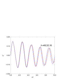
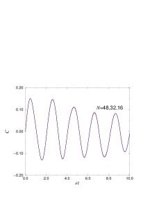
Figure 1: Chern-Simons number $C$ for three values of the cutoff, $N=16,32,48$ and G/e = 0.5. Left: the bare $v_{B}^{2}=10$ is kept fixed. Right: the renormalized $v_{R}^{2}=11.25$ is kept fixed.

The equations contain the ultraviolet divergences of the quantum theory, and need to be renormalized. In the full quantum theory only the scalar self energy is divergent, and because we only integrated out the fermions, we expect to find only the fermion loop contribution. Let’s take a closer look to the scalar field equation (2). If we take for simplicity $\phi=v_{R}/\sqrt{2}$ (i.e. equal to the renormalized v.e.v., $v_{B}$ is the bare parameter), and $A_{1}=0$, and also evaluate the fermions in this background, (2) reduces to the gap equation

$$\lambda(v_{R}^{2}-v_{B}^{2})\frac{v_{R}}{\sqrt{2}}=G\langle F\rangle(v_{R}),\;\;\;\;\langle F\rangle(v_{R})=\frac{Gv_{R}}{\sqrt{2}}\left(\frac{1}{\pi}\log N+{\cal O}(N_{0})\right).$$ (4)

An explicit calculation of $\langle F\rangle$ shows that it is indeed a logarithmically divergent sum, indicated with $\log N$ in (4b) ($N$ is the number of spatial lattice points). This divergence is canceled by the appropriate $v_{B}$. In practice, we fix $v_{R}$, and then find (for certain $N$, i.e. lattice spacing) the corresponding bare parameter $v_{B}$, from (4a). The result of this procedure is demonstrated in fig. 1. As expected, a proper renormalization gives converging physical results.

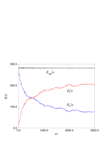
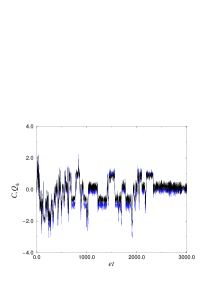
Figure 2: Left: Energy of the Bose fields, fermion field, and the conserved sum. Right: Chern-Simons number (dashed), and the anomalous charge (solid), for $G/e=0$.

In fig. 1, the Chern-Simons number undergoes a damped oscillation, with a small amplitude. Remember that the sphaleron sits at half-integer $C$. To probe this non-perturbative physics, we put more energy in the initial Bose fields. The results are shown in fig. 2. The initial state is clearly out-of-equilibrium and there is energy transfer from the Bose fields to the fermions. The Chern-Simons number is initially very wild, but as the bosonic energy decreases, the Bose fields start to feel the sphaleron barriers, and plateaus become visible. The anomalous charge follows the Chern-Simons number, in accordance with the anomaly equation: $\Delta Q_{5}=\Delta C$.

Energy transfer from the Bose fields to the fermionic degrees of freedom cannot go on forever because of Pauli blocking. This becomes clear if we choose the initial energy in the Bose fields to be much larger than before (compare figs. 2, 3). Again there is rapid energy transfer (until approx. $et=1000$), but then there is a rather sharp transition after which the energy in both subsystems remains approximately constant. A heuristic picture is as follows: the state with maximal fermion energy is given by a completely filled Dirac sea and sky. Note that this situation is not physical, it is a manifestation of the fact that for finite $N$ we only have a finite number of states. Nevertheless, a calculation of the ‘free’ fermion energy (i.e. neglecting the fluctuating Bose fields, keeping only $\phi=v_{R}/\sqrt{2}$) when all states in the spectrum are completely filled, gives for our choice of parameters and for $N=32$, $E_{f}^{\rm max}/e=815$. Indeed, a blowup shows that the fermion energy fluctuates around this value.

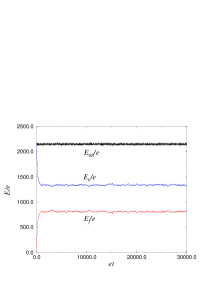
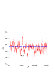
Figure 3: Left: as in fig. 2 (left), with $G/e=0.1$. Right: blowup of the fermion energy, the ‘free’ maximal fermion energy is indicated with a dashed line.

4 Summary

As an approximation to non-perturbative dynamics in quantum field theory, we studied a coupled system of classical Bose fields and a quantized fermion field. Skipping many technical details, we presented three numerical results. Many more questions can be addressed in this framework (e.g. long time behaviour, inclusion of CP violation, sphaleron rate in the presence of fermions), and we hope to report on these issues in the future.

References

References

- [1] F. Cooper, S. Habib, Y. Kluger, E. Mottola, J.P. Paz and P.R. Anderson, Phys. Rev. D50 (1994) 2848.
- [2] See e.g. F. Cooper, S. Habib, Y. Kluger and E. Mottola, Phys. Rev. D55 (1997) 6471; D. Boyanovsky et. al., Phys. Rev. D57 (1998) 2166; J. Baacke, K. Heitmann and C. Pätzold, Phys. Rev. D58 (1998) 125013; and references therein.
- [3] G. Aarts and J. Smit, hep-ph/9812413.