We study the helicity amplitudes of the process $\gamma\gamma\to\gamma\gamma$ at high energy, which in the standard and SUSY models first arise at the one-loop order. In the standard model (SM), the diagrams involve $W$ and charged quark and lepton loops, while in SUSY we also have contributions from chargino, charged sfermion and Higgs loop diagrams. The SUSY contributions are most important in the region above the threshold for producing the supersymmetric partners; since there, they interfere most effectively with the primarily imaginary SM amplitudes. Simple expressions for the relevant 1-loop functions are given, which provide a direct overview of the behaviour of the helicity amplitudes in the whole parameter space at high energies. The various characteristics of a large set of observables are studied in detail.

1 Introduction

A striking option for a the future $e^{+}e^{-}$ Linear Collider (LC) [1, 2], is to operate it as a $\gamma\gamma$ Collider ($LC_{\gamma\gamma}$) whose c.m. energy may be variable and as high as $80\%$ of the initial $e^{+}e^{-}$ c.m. energy [3]. According to the present ideas, this should be achieved by colliding each of the $e^{\pm}$ beams with laser photons, which are subsequently backscattered, through the Compton effect. This way, very energetic photons along the $e^{\pm}$ direction are generated, while $e^{\pm}$ loose most of their energy [3, 4]. The energy spectrum and spin composition of the two photon beams, in the thus generated $\gamma\gamma$ Collider, depend of course on the energies and polarization conditions of the $e^{\pm}$ beams and lasers. At present, there are still many technical details to overcome, before deciding that such an option is really viable [4]. In this respect, it is necessary to assess its importance, before deciding whether the physics opportunities there, justify the effort.

Up to now it has been seen in many cases that $LC_{\gamma\gamma}$ is more powerful than LC, in searching for New Physics (NP) beyond the Standard Model (SM); mainly because the $\gamma\gamma$ initial state has the tendency to couple stronger than the $e^{+}e^{-}$ one, to the new degrees of freedom contained in many forms of NP [5, 6]. Such searches may involve either the direct production of new degrees of freedom (like e.g. charginos, light sleptons or a light $\tilde{t}_{1}$ (stop) in SUSY models) [7]; or the precise study of the production of SM particles like e.g.  in $\gamma\gamma\to W^{+}W^{-},~{}H$ or the production of Higgs pairs, where the new degrees of freedom contribute virtually, in some loop diagrams [1, 5, 6, 7].

In this respect, processes like $\gamma\gamma\to\gamma\gamma$, $\gamma\gamma\to Z\gamma$, $\gamma\gamma\to ZZ$ should also provide very important tools for searching or constraining NP; particularly because the SM contribution there, first appears at the 1-loop level and should be small. In the present paper, we concentrate on the $\gamma\gamma\to\gamma\gamma$ process, which in SM is fully determined by the contributions of charged fermion and $W$ loops. The $W$-loop contribution has been first calculated in [8] in terms of the standard 1-loop functions of [9], while the expression for the fermion contribution in terms of the same functions has been given in [10].

The structure of the $\gamma\gamma\to\gamma\gamma$ helicity amplitudes at high energies ($\sqrt{s_{\gamma\gamma}}\gtrsim 0.3~{}TeV$) and any scattering angle, turns out to be remarkably simple and intuitive. In the Standard Model, the whole process is dominated at high energies, by the helicity non-flip amplitudes $F_{\pm\pm\pm\pm}(s,t,u)$ and $F_{\pm\mp\pm\mp}(s,t,u)=F_{\pm\mp\mp\pm}(s,u,t)$, which are predominantly imaginary for all scattering angles [8, 11]. The dominant contribution to these amplitudes for $\sqrt{s_{\gamma\gamma}}\gtrsim 0.3~{}TeV$, is easily identified to come from the $W$ loop. We could remark, in passing, that the $\gamma\gamma\to\gamma\gamma$ amplitude at high energies has exactly the structure anticipated long ago by combining the Vector Meson Dominance (VMD) idea, with the assumption that the Pomeron couplings are predominantly helicity-non-flip! But, of course in the present theory, the role of the Pomeron is played by the $W$ loop, and the aforementioned success of VMD seems accidental!

As it has been recently emphasized in [11], this remarkable property suggests to use the $\gamma\gamma\to\gamma\gamma$ scattering process as a tool for searching for types of new physics characterized by amplitudes with a substantial imaginary part; like e.g.  effects due to chargino or charged slepton loop diagrams above the threshold; $s$-channel resonance production; or new strong interactions inducing unitarity saturating contributions to the NP amplitudes.

In the present paper we study in detail the $\gamma\gamma\to\gamma\gamma$ amplitudes in the standard and SUSY models. The idea behind this, is to use $\gamma\gamma\to\gamma\gamma$ scattering for searching for SUSY signatures. The situation for such a search should be particularly favorable at energies above the charged supersymmetric particle threshold, where the SUSY contribution to the $\gamma\gamma\to\gamma\gamma$ amplitude has a large imaginary part interfering effectively with the standard one. Such a search is complementary to the direct production of charged SUSY particles and it should help identifying their nature; since it avoids the model-dependent task of studying their decay modes, once they are actually produced. More explicitly: the charged sparticle loop contribution to $\gamma\gamma\to\gamma\gamma$, is independent of the many parameters entering their decay modes and determining e.g.  the soft SUSY breaking and the possible $R$-parity violating sectors.

The expressions for the $W$ and fermion loop contributions are of course well known [8, 10], but their detailed properties had not been fully analyzed before. We have confirmed the results of [8, 10], using the non-linear gauge of [12], and we give them in Appendix A, together with the 1-loop contribution induced by a single charged scalar particle. The rest of the contents of the paper is the following: In Section 2, a simple and accurate high energy approximation to the SM $\gamma\gamma\to\gamma\gamma$ amplitude is presented, which elucidates very clearly its physical properties in SM at high energies, and should be useful for identifying certain forms of New Physics (NP) contributing to it. We consider SUSY, as an example of such an NP, and we discuss the physical properties of the contribution to the above amplitudes from a chargino or charged slepton; which may be expected to be lighter than $\sim 250$GeV [2]. In Sec. 3, we study the $\gamma\gamma\to\gamma\gamma$ cross sections in the standard and SUSY models, for various polarizations of the incoming photons. We identify the sensitivity of these cross sections to various SUSY effects and we discuss their observability in unpolarized and polarized $\gamma\gamma$ collisions, realized through the present ideas of laser backscattering. In Appendix B we summarize the laser backscattering formalism and give the expressions of the $\gamma\gamma$ flux and the two-photon spin density matrix [3]. Finally, in Sec. 4, we summarize the results and give our conclusions.

2 An overall view of the $\gamma\gamma\to\gamma\gamma$ amplitudes.

The invariant helicity amplitudes $F_{\lambda_{1}\lambda_{2}\lambda_{3}\lambda_{4}}(\hat{s},\hat{t},\hat{u})$ for the process $\gamma\gamma\to\gamma\gamma$ are given in Appendix A. Altogether there are $2^{4}=16$ helicity amplitudes, which must of course satisfy the constraints from Bose (A.3, A.2) and crossing symmetry (A.4, A.5). In SM or SUSY models, parity and time inversion invariance also hold, which imply (A.6)) and (A.7) respectively, thereby allowing to express all helicity amplitudes in terms of the analytic expressions of just the three functions $F_{+++-}(\hat{s},\hat{t},\hat{u})$, $F_{++--}(\hat{s},\hat{t},\hat{u})$ and $F_{++++}(\hat{s},\hat{t},\hat{u})$ [8]; compare (A.8 - A.11). In Appendix A, we reproduce the $W$ and charged fermion contributions of [8] and [10] respectively, and we also give the charged scalar loop contributions to these amplitudes.

All results are given in terms of the standard 1-loop functions $B_{0}$, $C_{0}$ and $D_{0}$, first introduced in [9]. For the special photon scattering case we are interested in, these functions may be written as $B_{0}(s)$, $C_{0}(s)$, $D_{0}(s,t)$, following the definitions in (A.12 - A.14). These functions depend only on the indicated variables and the mass $m$ of the particle circulating in the loop. In the SM case, the role of the mass $m$ is played by either $W$ mass or the masses of the quarks and charged leptons. This means that in the kinematical region relevant for a Linear Collider, we have $\hat{s},|\hat{t}|,|\hat{u}|\gg m^{2}$; apart of course from the $t$-quark case, which is not very important for the overall magnitude. It turns out that for high $(\hat{s},|\hat{t}|,|\hat{u}|)$, an excellent approximation to the above 1-loop functions is given by

$$B_{0}(\hat{s}) \simeq \Delta+2-Ln\left(\frac{-\hat{s}-i\epsilon}{\mu^{2}}\right)\ ~{},$$ (1)

$$C_{0}(\hat{s}) \simeq \frac{1}{2\hat{s}}\left[Ln\left(\frac{-\hat{s}-i\epsilon}{m^{2}}\right)\right]^{2}\ \ ,$$ (2)

$$D_{0}(\hat{s},\hat{t}) \simeq \frac{2}{\hat{s}\hat{t}}\Bigg{[}Ln\left(\frac{-\hat{s}-i\epsilon}{m^{2}}\right)Ln\left(\frac{-\hat{t}-i\epsilon}{m^{2}}\right)-~{}\frac{\pi^{2}}{2}\Bigg{]}\ \ ,$$ (3)

where $\Delta$ is the usual infinite term entering the calculation of the divergent integral for $B_{0}(\hat{s})$, and $\mu$ is the dimensional regularization parameter [16]. These results can be easily obtained by keeping the leading term in a $m^{2}/\hat{s},~{}m^{2}/\hat{t}$ expansion of the formulae in the Appendix of [13]. Numerically they are extremely accurate, provided that $|\hat{s}|\gtrsim 100~{}m^{2}$ in (1, 2); while a similar accuracy for (3) obtains in the region

$$-\hat{s}\gtrsim 100~{}m^{2}~{}~{}~{} ,~{}~{}~{}~{}-\hat{t}\gtrsim 100~{}m^{2}~{}~{}~{},$$ (4)

or $$~{}~{}~{}~{}~{}\hat{s}>-\hat{t}\gtrsim 100~{}m^{2}~{}~{}~{},~{}~{}~{}~{}~{}$$

or $$~{}~{}~{}~{}~{}\hat{t}>-\hat{s}\gtrsim 100~{}m^{2}\ \ .$$

We can now obtain simple expressions for the $W$ and light fermion contributions to the $\gamma\gamma\to\gamma\gamma$ amplitudes, which should be quite accurate for the large energies and scattering angles relevant for $LC_{\gamma\gamma}$ experiments. Substituting thus, (1 - 3) in (A.15 - A.17) and neglecting all terms of order $m_{W}^{2}/\hat{s}$, $m_{W}^{2}/\hat{t}$, $m_{W}^{2}/\hat{u}$, we get

$$\frac{F^{W}_{++++}(\hat{s},\hat{t},\hat{u})}{\alpha^{2}}\simeq 12+12~{}\left(\frac{\hat{u}-\hat{t}}{\hat{s}}\right)\left\{Ln\left(\frac{-\hat{u}-i\epsilon}{m^{2}}\right)-Ln\left(\frac{-\hat{t}-i\epsilon}{m^{2}}\right)\right\}$$

$$+16\left(1-~{}\frac{3\hat{t}\hat{u}}{4\hat{s}^{2}}\right)\Bigg{[}\left\{Ln\left(\frac{-\hat{u}-i\epsilon}{m^{2}}\right)-Ln\left(\frac{-\hat{t}-i\epsilon}{m^{2}}\right)\right\}^{2}+\pi^{2}\Bigg{]}$$

$$+16\hat{s}^{2}\Bigg{\{}\frac{1}{\hat{s}\hat{t}}\,Ln\left(\frac{-\hat{s}-i\epsilon}{m^{2}}\right)Ln\left(\frac{-\hat{t}-i\epsilon}{m^{2}}\right)+\frac{1}{\hat{s}\hat{u}}\,Ln\left(\frac{-\hat{s}-i\epsilon}{m^{2}}\right)Ln\left(\frac{-\hat{u}-i\epsilon}{m^{2}}\right)$$

$$+\frac{1}{\hat{t}\hat{u}}\,Ln\left(\frac{-\hat{t}-i\epsilon}{m^{2}}\right)Ln\left(\frac{-\hat{u}-i\epsilon}{m^{2}}\right)\Bigg{\}}~{}~{},$$ (5)

$$F^{W}_{+++-}(\hat{s},\hat{t},\hat{u})\simeq F^{W}_{++--}(\hat{s},\hat{t},\hat{u})\simeq-12\alpha^{2}\simeq\mbox{negligible}~{}~{}.$$ (6)

Correspondingly, the asymptotic expressions for a single fermion loop of charge $Q_{f}$ and mass $m_{f}$, derived from (A.18 - A.20) by neglecting all terms of $O(m_{f}^{2}/\hat{s})$, $O(m_{f}^{2}/\hat{t})$, $O(m_{f}^{2}/\hat{u})$, are

$$\frac{F^{f}_{++++}(\hat{s},\hat{t},\hat{u})}{\alpha^{2}Q_{f}^{4}}\simeq-8-8~{}\left(\frac{\hat{u}-\hat{t}}{\hat{s}}\right)\left\{Ln\left(\frac{-\hat{u}-i\epsilon}{m^{2}}\right)-Ln\left(\frac{-\hat{t}-i\epsilon}{m^{2}}\right)\right\}$$

$$-4~{}\frac{(\hat{t}^{2}+\hat{u}^{2})}{\hat{s}^{2}}\Bigg{[}\left\{Ln\left(\frac{-\hat{u}-i\epsilon}{m^{2}}\right)-Ln\left(\frac{-\hat{t}-i\epsilon}{m^{2}}\right)\right\}^{2}+\pi^{2}\Bigg{]}~{}~{},$$ (7)

$$F^{f}_{+++-}(\hat{s},\hat{t},\hat{u})\simeq F^{f}_{++--}(\hat{s},\hat{t},\hat{u})\simeq 8Q_{f}^{4}\alpha^{2}\simeq\mbox{negligible}~{}~{}.$$ (8)

On the basis of (5 - 8) and (A.8 - A.11), we see that in the Standard Model, the only physical amplitudes which have a chance of being non-negligible at LC energies, are $F_{\pm\pm\pm\pm}(\hat{s},\hat{t},\hat{u})$ and $F_{\pm\mp\pm\mp}(\hat{s},\hat{t},\hat{u})=F_{\pm\mp\mp\pm}(\hat{s},\hat{u},\hat{t})$. Indeed a detail look at the aforementioned equations shows that these are the only amplitudes which (may generally) receive a logarithmically enhanced high energy contribution. In the physical region of the scattering amplitudes, such a contribution is almost purely imaginary and arises from the term within the last curly brackets of the $W$ loop expression (5).

The real contributions to the various amplitudes are much smaller. For the physical amplitude $F_{\pm\pm\pm\pm}$, the most important real contribution below $1~{}TeV$, arises from the last term in (7). Its origin is fermionic and it is enhanced not by a logarithm, but rather by a large $\pi^{2}$ term. In this energy range, there exist also a somewhat smaller real contribution affecting the $F_{\pm\pm\pm\pm}(\hat{s},\hat{t},\hat{u})$ and $F_{\pm\mp\pm\mp}(\hat{s},\hat{t},\hat{u})=F_{\pm\mp\mp\pm}(\hat{s},\hat{u},\hat{t})$ amplitudes, which is due to some linear $log$ terms; while the Sudakov-type $log^{2}$ terms cancel out at both, large ($\hat{s}\sim-\hat{t}/2\sim-\hat{u}/2$) and small angles ($\hat{s}\gg-\hat{t}$ or $\hat{s}\gg-\hat{u}$. In any case, it should be noted, that the real part of all the large amplitudes is always more than five times smaller than the imaginary part.

Numerical results for these amplitudes using the exact 1-loop functions have been presented in Fig.1 of [11], and they are quite similar to the results obtained from (5 - 8). Concerning the accuracy of the above asymptotic expressions at $LC_{\gamma\gamma}$ energies, we note that for the large amplitudes cases of $F_{++++}$ and $F_{+-+-}=F_{+--+}$, the asymptotic expressions tend to be higher than the exact 1-loop ones by $\sim 20\%$ at about $0.4~{}TeV$, and by less than $10\%$ as we approach $1~{}TeV$. For the small amplitudes cases, the relative accuracy may occasionally be not so good, but this is not relevant, since they are really negligible. To complete the discussion about the SM amplitudes, we also note that the top contribution is at least an order of magnitude smaller than the other SM contributions we have just discussed.

The approximate SM amplitudes in (5 - 8) can then be used to understand the magnitude of the NP contribution to the $\gamma\gamma\to\gamma\gamma$ cross sections, under various polarizations conditions. These suggest that $\gamma\gamma\to\gamma\gamma$ scattering may provide a very useful tool for searching for types of New Physics (NP), with largely imaginary amplitudes [11].

Thus in Fig.1a,b we give the contributions from a chargino of mass 100 GeV for two values of the c.m. scattering angle, derived from (A.18 -A.20), on the basis of the exact expressions for the 1-loop functions [14]. The corresponding results for a slepton, are derived using (A.21 - A.23) and presented in Fig.1c,d. As seen in both cases, immediately above the threshold, a considerable imaginary contribution to the $F_{++++}$ amplitude starts developing, which can interfere with the SM one and produce a measurable effect. We also note, that the slepton contribution is considerably smaller than the chargino one, but, as we will see below, the effect may increase if several scalar sparticles (charged sleptons, $\tilde{t}_{1}$ or $\tilde{H}^{+}$) appear below $250GeV$.

3 The $\gamma\gamma\to\gamma\gamma$ Cross sections

We next explore the possibility to use polarized or unpolarized $\gamma\gamma$ collisions in an LC operated in the $\gamma\gamma$ mode, through laser backscattering [15, 11]. Bose statistics and the assumption of Parity invariance leads to the following form for the $\gamma\gamma\to\gamma\gamma$ cross section

$${d\sigma\over d\tau d\cos\vartheta^{*}} = {d\bar{L}_{\gamma\gamma}\over d\tau}\Bigg{\{}{d\bar{\sigma}_{0}\over d\cos\vartheta^{*}}+\langle\xi_{2}\xi_{2}^{\prime}\rangle{d\bar{\sigma}_{22}\over d\cos\vartheta^{*}}+[\langle\xi_{3}\rangle\cos 2\phi+\langle\xi_{3}^{\prime}\rangle\cos 2\phi^{\prime}]{d\bar{\sigma}_{3}\over d\cos\vartheta^{*}}$$ (9)

$$+\langle\xi_{3}\xi_{3}^{\prime}\rangle[{d\bar{\sigma}_{33}\over d\cos\vartheta^{*}}\cos 2(\phi+\phi^{\prime})+{d\bar{\sigma}^{\prime}_{33}\over d\cos\vartheta^{*}}\cos 2(\phi-\phi^{\prime})]$$

$$+[\langle\xi_{2}\xi_{3}^{\prime}\rangle\sin 2\phi^{\prime}-\langle\xi_{3}\xi_{2}^{\prime}\rangle\sin 2\phi]{d\bar{\sigma}_{23}\over d\cos\vartheta^{*}}\Bigg{\}}\ \ ,$$

where

$${d\bar{\sigma}_{0}\over d\cos\vartheta^{*}} = \left({1\over 128\pi\hat{s}}\right)\sum_{\lambda_{3}\lambda_{4}}[|F_{++\lambda_{3}\lambda_{4}}|^{2}+|F_{+-\lambda_{3}\lambda_{4}}|^{2}]~{},$$ (10)

$${d\bar{\sigma}_{22}\over d\cos\vartheta^{*}} = \left({1\over 128\pi\hat{s}}\right)\sum_{\lambda_{3}\lambda_{4}}[|F_{++\lambda_{3}\lambda_{4}}|^{2}-|F_{+-\lambda_{3}\lambda_{4}}|^{2}]\ ,$$ (11)

$${d\bar{\sigma}_{3}\over d\cos\vartheta^{*}} = \left({-1\over 64\pi\hat{s}}\right)\sum_{\lambda_{3}\lambda_{4}}Re[F_{++\lambda_{3}\lambda_{4}}F^{*}_{-+\lambda_{3}\lambda_{4}}]\ ,$$ (12)

$${d\bar{\sigma}_{33}\over d\cos\vartheta^{*}} = \left({1\over 128\pi\hat{s}}\right)\sum_{\lambda_{3}\lambda_{4}}Re[F_{+-\lambda_{3}\lambda_{4}}F^{*}_{-+\lambda_{3}\lambda_{4}}]\ ,$$ (13)

$${d\bar{\sigma}^{\prime}_{33}\over d\cos\vartheta^{*}} = \left({1\over 128\pi\hat{s}}\right)\sum_{\lambda_{3}\lambda_{4}}Re[F_{++\lambda_{3}\lambda_{4}}F^{*}_{--\lambda_{3}\lambda_{4}}]\ ,$$ (14)

$${d\bar{\sigma}_{23}\over d\cos\vartheta^{*}} = \left({1\over 64\pi\hat{s}}\right)\sum_{\lambda_{3}\lambda_{4}}Im[F_{++\lambda_{3}\lambda_{4}}F^{*}_{+-\lambda_{3}\lambda_{4}}]\ ,$$ (15)

are expressed in terms of the $\gamma\gamma\to\gamma\gamma$ amplitudes given in Appendix A. Note that only $d\bar{\sigma}_{0}/d\cos\vartheta^{*}$ is positive definite.

The quantity $d\bar{L}_{\gamma\gamma}/d\tau$ (compare (9), (B.14)) describes the photon-photon luminosity per unit $e^{-}e^{+}$ flux, in an LC operated in the $\gamma\gamma$ mode [3]. Moreover, $\vartheta^{*}$ is the scattering angle in the $\gamma\gamma$ rest frame and $\tau\equiv s_{\gamma\gamma}/s_{ee}$. The Stokes parameters $\xi_{2}$, $\xi_{3}$ and the azimuthal angle $\phi$ in (9), determine the normalized helicity density matrix of one of the backscattered photons $\rho^{BN}_{\lambda\lambda^{\prime}}$ through the formalism in Appendix B; compare (B.4) [15]. The corresponding parameters for the other backscattered photon are denoted by a prime.

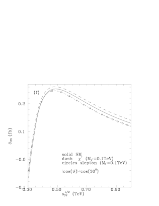
Figure 2: $\bar{\sigma}_{33}^{\prime}$ and $\bar{\sigma}_{23}$ for SM (solid) and in the presence of a chargino (dash) or a charged slepton (circles) contribution.

The results for the cross sections $\bar{\sigma}_{j}$, integrated in the range $30^{0}\leq\vartheta^{*}\leq 150^{0}$, are given in Fig.2a-f, for the standard model, as well as for the case including the contributions from a single chargino or a single charged slepton with mass 100 GeV. In Fig.3a-f the corresponding results for a 250 GeV SUSY mass are given. Note that the charged slepton results will also be valid for the charged Higgs case; while for a single $\tilde{t}$ contribution, the SUSY effect will be reduced by a factor $3Q^{4}_{\tilde{t}}=3(2/3)^{4}\simeq 0.59$. As seen from Fig.2a-f,3a-f, the chargino and slepton contributions to $\bar{\sigma}_{3}$ and $\bar{\sigma}_{33}^{\prime}$ are mostly of opposite sign; as opposed to the $\bar{\sigma}_{0}$, $\bar{\sigma}_{22}$ and $\bar{\sigma}_{33}$ cases where the signs are usually the same. For $\bar{\sigma}_{23}$ an intermediate situation appears, in which the chargino and slepton contributions tend to be of opposite sign for $M_{\chi}\sim M_{\tilde{l}}\sim 100GeV$, but they are mostly of the same sign if $M_{\chi}\sim M_{\tilde{l}}\sim 250GeV$; compare Fig.2f,3f.

Unfortunately, as seen from Fig.2c,e and Fig.3c,e, the quantities $\bar{\sigma}_{3}$ and $\bar{\sigma}_{33}^{\prime}$, which are most sensitive to the nature of the contributing sparticles, are numerically the smallest ones. For studying therefore SUSY-type NP, we have to rely mainly on the largest quantity $\bar{\sigma}_{0}$ appearing in Fig.2a. Depending on the experimental situation though, $\bar{\sigma}_{22}$ given in Fig.2b, should also prove useful. This, of course, should not lead us to the idea that those $\bar{\sigma}_{j}$, which are small in SM and SUSY, are not interesting; since there may exist other forms of NP for which they are sizable. It would therefore be important to study them and bound their magnitude, in order to check at least the consistency with SM and/or SUSY.

To get a feeling of the observability of the various quantities $\bar{\sigma}_{j}$ appearing in (9), we next turn to the experimental aspects of the $\gamma\gamma$ collision process realized through the laser backscattering [1, 3]. The general form of the overall luminosity $d\bar{L}_{\gamma\gamma}/d\tau$ and of the density matrix of the photon pair, are given in Appendix B; based on the assumption that the conversion point where the Compton backscattering occurs, coincides with the interaction point at which the $\gamma\gamma$ collision takes place [3]. It should be noticed that $d\bar{L}_{\gamma\gamma}/d\tau$ depends on the frequencies, of the two lasers, through the parameters $x_{0}$ and $x_{0}^{\prime}$ of (B.5); and on the product of longitudinal $e^{\pm}$ and laser polarizations $P_{e}P_{\gamma}$ and $P_{e}^{\prime}P_{\gamma}^{\prime}$. As a result, $d\bar{L}_{\gamma\gamma}/d\tau$ becomes harder as $P_{e}P_{\gamma}\to-1$, or as $x_{0}$ or $x_{0}^{\prime}$ approach their maximum value $2(1+\sqrt{2})$; (compare Fig.4).

For obtaining the number of the expected events in each case, the cross sections in (9) should be multiplied by the $e^{+}e^{-}$ luminosity ${\cal L}_{ee}$, whose presently contemplated value for the LC project is ${\cal L}_{ee}\simeq 500~{}-~{}1000~{}fb^{-1}$ per one or two years of running in e.g. the high luminosity TESLA mode at energies of $350-800~{}GeV$ [1].

To this aim, we first express $\bar{\sigma}_{j}$, multiplied by their $\gamma\gamma$ luminosity coefficient in (9), in terms of linear combinations of cross sections for various longitudinal and/or transverse polarizations of the $e^{\pm}$ and laser beams. Thus, for unpolarized $e^{\pm}$ and laser beams, $\bar{\sigma}_{0}$ can be measured through

$$\left(\frac{d\bar{L}_{\gamma\gamma}}{d\tau}\right){d\bar{\sigma}_{0}\over d\cos\vartheta^{*}}={d\sigma\over d\tau d\cos\vartheta^{*}}\Bigg{|}_{\mbox{unpol}}~{}~{}~{}~{}\ .$$ (16)

On the other hand, by considering collisions with the combinations of longitudinal polarizations $(P_{e},P_{\gamma},P_{e}^{\prime},P_{\gamma}^{\prime})$ and $(P_{e},P_{\gamma},-P_{e}^{\prime},-P_{\gamma}^{\prime})$ and no transverse polarizations, the quantities $\bar{\sigma}_{0}$ and $\bar{\sigma}_{22}$ can be measured through

$$\left({d\bar{L}_{\gamma\gamma}\over d\tau}\right){d\bar{\sigma}_{0}\over d\cos\vartheta^{*}}=\frac{1}{2}\Bigg{[}{d\sigma(P_{e},P_{\gamma},P_{e}^{\prime},P_{\gamma}^{\prime})\over d\tau d\cos\vartheta^{*}}+{d\sigma(P_{e},P_{\gamma},-P_{e}^{\prime},-P_{\gamma}^{\prime})\over d\tau d\cos\vartheta^{*}}\Bigg{]}\ ,$$ (17)

$$\left({d\bar{L}_{\gamma\gamma}\over d\tau}\right)\langle\xi_{2}\xi_{2}^{\prime}\rangle{d\bar{\sigma}_{22}\over d\cos\vartheta^{*}}=\frac{1}{2}\Bigg{[}{d\sigma(P_{e},P_{\gamma},P_{e}^{\prime},P_{\gamma}^{\prime})\over d\tau d\cos\vartheta^{*}}-{d\sigma(P_{e},P_{\gamma},-P_{e}^{\prime},-P_{\gamma}^{\prime})\over d\tau d\cos\vartheta^{*}}\Bigg{]}\ .$$ (18)

The results of (16 - 18) integrated in the region $30^{0}\leq\vartheta^{*}\leq 150^{0}$, for the indicated polarizations and the laser parameters $x_{0}=x_{0}^{\prime}=4.83$, are presented in Fig.5 for a $100~{}GeV$ chargino or slepton.

The measurement of $\bar{\sigma}_{3}$ could be achieved by selecting one of the two laser photons to be purely transversely polarized with e.g.  $P_{t}=1$ and direction determined by the azimuthal angle $\phi$, while the other laser photon is taken unpolarized. In this case $\bar{\sigma}_{3}$, together with $\bar{\sigma}_{0}$, may be determined through

$$2\langle\xi_{3}\rangle\,\left({d\bar{L}_{\gamma\gamma}\over d\tau}\right){d\bar{\sigma}_{3}\over d\cos\vartheta^{*}} = {d\sigma(\phi=0)\over d\tau d\cos\vartheta^{*}}~{}-~{}{d\sigma(\phi=\pi/2)\over d\tau d\cos\vartheta^{*}}\ ,$$ (19)

$$2\,\left({d\bar{L}_{\gamma\gamma}\over d\tau}\right){d\bar{\sigma}_{0}\over d\cos\vartheta^{*}} = {d\sigma(\phi=0)\over d\tau d\cos\vartheta^{*}}~{}+~{}{d\sigma(\phi=\pi/2)\over d\tau d\cos\vartheta^{*}}\ .$$ (20)

If both laser photons are purely transversely polarized, with $P_{t}=P_{t}^{\prime}=1$ and their directions determined by the respective azimuthal angles $\phi,~{}\phi^{\prime}$; then $\bar{\sigma}_{3}$, $\bar{\sigma}_{33}$, $\bar{\sigma}_{33}^{\prime}$, together with $\bar{\sigma}_{0}$ can be determined through

$$2\left({d\bar{L}_{\gamma\gamma}\over d\tau}\right){d\bar{\sigma}_{0}\over d\cos\vartheta^{*}} = {d\sigma(\phi=0,\phi^{\prime}=\pi/4)\over d\tau d\cos\vartheta^{*}}+{d\sigma(\phi=\pi/4,\phi^{\prime}=\pi/2)\over d\tau d\cos\vartheta^{*}}\ ,$$ (21)

$$(\langle\xi_{3}\rangle+\langle\xi_{3}^{\prime}\rangle)\left({d\bar{L}_{\gamma\gamma}\over d\tau}\right){d\bar{\sigma}_{3}\over d\cos\vartheta^{*}} = {d\sigma(\phi=0,\phi^{\prime}=\pi/4)\over d\tau d\cos\vartheta^{*}}-{d\sigma(\phi=\pi/4,\phi^{\prime}=\pi/2)\over d\tau d\cos\vartheta^{*}}\ ,$$ (22)

$$2\langle\xi_{3}\xi_{3}^{\prime}\rangle\left({d\bar{L}_{\gamma\gamma}\over d\tau}\right){d\bar{\sigma}_{33}\over d\cos\vartheta^{*}} = {d\sigma(\phi=0,\phi^{\prime}=0)\over d\tau d\cos\vartheta^{*}}-{d\sigma(\phi=0,\phi^{\prime}=\pi/4)\over d\tau d\cos\vartheta^{*}}$$ (23)

$$- {d\sigma(\phi=\pi/4,\phi^{\prime}=0)\over d\tau d\cos\vartheta^{*}}+{d\sigma(\phi=\pi/4,\phi^{\prime}=-\pi/4)\over d\tau d\cos\vartheta^{*}},$$

$$2\langle\xi_{3}\xi_{3}^{\prime}\rangle\left({d\bar{L}_{\gamma\gamma}\over d\tau}\right){d\bar{\sigma}_{33}^{\prime}\over d\cos\vartheta^{*}} = {d\sigma(\phi=0,\phi^{\prime}=0)\over d\tau d\cos\vartheta^{*}}-{d\sigma(\phi=0,\phi^{\prime}=\pi/4)\over d\tau d\cos\vartheta^{*}}$$ (24)

$$- {d\sigma(\phi=\pi/4,\phi^{\prime}=0)\over d\tau d\cos\vartheta^{*}}\ +{d\sigma(\phi=\pi/4,\phi^{\prime}=+\pi/4)\over d\tau d\cos\vartheta^{*}}.$$

The results of (21 - 24), integrated in the region $30^{0}\leq\vartheta^{*}\leq 150^{0}$, for the indicated polarizations and SUSY masses are presented in Fig.6. In order to increase sensitivity as much as possible, we have chosen $x_{0}=x_{0}^{\prime}=1$, which has the side effect of making the $\gamma\gamma$ spectrum softer; (compare Fig.4).

Finally, for studying $\bar{\sigma}_{23}$, we need a mixed polarization situation, where one laser photon is longitudinally polarized, while the other is transverse; like e.g. ($P_{e}=0.8$, $P_{\gamma}=-1$, $P_{t}=0$) for the one, and ($P_{e}^{\prime}=P_{\gamma}^{\prime}=0$, $P_{t}^{\prime}=1$ with direction defined by $\phi^{\prime}$) for the other. To optimize the flux spectrum $d\bar{L}_{\gamma\gamma}/d\tau$, it may be better to choose $x_{0}\not=x_{0}^{\prime}$ in this case. In such case we have

$$2\left({d\bar{L}_{\gamma\gamma}\over d\tau}\right){d\bar{\sigma}_{0}\over d\cos\vartheta^{*}} = {d\sigma(\phi^{\prime}=\pi/4)\over d\tau d\cos\vartheta^{*}}+{d\sigma(\phi^{\prime}=3\pi/4)\over d\tau d\cos\vartheta^{*}}\ ,$$ (25)

$$2\langle\xi_{2}\xi_{3}^{\prime}\rangle\left({d\bar{L}_{\gamma\gamma}\over d\tau}\right){d\bar{\sigma}_{23}\over d\cos\vartheta^{*}} = {d\sigma(\phi^{\prime}=\pi/4)\over d\tau d\cos\vartheta^{*}}-{d\sigma(\phi^{\prime}=3\pi/4)\over d\tau d\cos\vartheta^{*}}\ ,$$ (26)

and an example appears in Fig.7. In this figure we also give predictions for an alternative measurement of $\bar{\sigma}_{3}$; compare Fig.6b and Fig.7b.

Using ${\cal L}_{ee}=500fb^{-1}$, then the $100~{}GeV$ chargino effect indicated in Fig.5a for a $350~{}GeV$ LC and unpolarized $e^{\pm}$ and laser beams, is at the 2.3 standard deviations (SD) level; while for the situation at Fig.5b, it increases 2.9 SD. In both cases, the effect arises from a $\bar{\sigma}_{0}$ measurement, which itself measures the unpolarized cross section. Nevertheless though, the sensitivity, as expressed by the number of SD, does depend on the polarizations and $x_{0}$ parameters, since these affect the $\gamma\gamma$ flux through $d\bar{L}_{\gamma\gamma}/d\tau$; (compare (B.14)). For studying therefore a suspected (due to some other signals) chargino of a certain mass, through $\gamma\gamma\to\gamma\gamma$ scattering, it will be important to optimize the LC and laser energies and $x_{0}$ parameters. To further elucidate this, we remark that for the situations in Fig.6a and Fig.7a, the chargino sensitivity is at the 3.9 SD and 4.2 SD respectively. In all cases, the $\tau$ regions used in estimating SD, are those employed in the corresponding figures.

For the same $100~{}GeV$ chargino as above, the $\bar{\sigma}_{22}$ effect in Fig.5c is at the 0.8 SD level, when a bin like $0.49\leq\tau\leq 0.62$ is used. Thus, a $\bar{\sigma}_{22}$ measurement, which necessitates linear polarization, can give an additional constraint.

The quantities $\bar{\sigma}_{3}$ $\bar{\sigma}_{33}$ $\bar{\sigma}_{33}^{\prime}$ and $\bar{\sigma}_{23}$ are too small to be measured with the above $\gamma\gamma$ flux, and the best we can hope for, is to put some reasonable bound on them, which could help excluding possible extreme forms of NP.

An analysis of the statistics of a $\bar{\sigma}_{0}$ measurement for a $150~{}GeV$ and $250~{}GeV$ chargino was also made, and in these cases we found that sensitivities at the 3 SD and 1.2 SD level should be respectively expected.

As an example of the charged scalar case within the loop, we considered the case of a single charged slepton. If its mass is in the $100~{}GeV$ range, then the results in Fig.5a,b, 6a, 7a would indicate a signal at the (0.5-0.7)SD level.

The situation may improve considerably though, if several, or even all six charged sleptons expected in the minimal SUSY model, and maybe also the lightest stop $\tilde{t}_{1}$ together with one chargino, lie in (100-250) GeV mass region [2]. A clearly measurable increase (compared to the SM prediction), may then appear in an $\bar{\sigma}_{0}$ measurement. This is concluded from Figs.2a, 3a, which show that in the (100-250)GeV mass range, a fermion and scalar charged particle loop contribute with the same sign to $\bar{\sigma}_{0}$.

4 Conclusions

In this paper we have offered a detailed analysis of the helicity amplitudes of the process $\gamma\gamma\to\gamma\gamma$ at high energies, and studied also the unpolarized and polarized cross section.

The spectacular property of the Standard Model prediction for this process is that, for energies above $0.3~{}TeV$, there only two independent helicity amplitudes which are important; namely $F_{\pm\pm\pm\pm}(\hat{s},\hat{t},\hat{u})$ and $F_{\pm\mp\pm\mp}(\hat{s},\hat{t},\hat{u})=F_{\pm\mp\mp\pm}(\hat{s},\hat{u},\hat{t})$. These amplitudes are helicity conserving and almost purely imaginary for all scattering angles. This property makes the $\gamma\gamma\to\gamma\gamma$ process an excellent tool for searching for types of new physics inducing large imaginary parts to such amplitudes.

As such, we have studied here the particular SUSY case of a single chargino or charged slepton contribution, at energies above the threshold for their actual production. These contributions depend of course only on the mass, charge and spin of the SUSY partners, and are independent of the many model-dependent parameters entering their decay modes. Thus, the study of the $\gamma\gamma\to\gamma\gamma$ cross sections should offer complementary information, to the one obtained from direct SUSY production cross sections.

For an LC collider at energies of $(350-800)GeV$ and a luminosity ${\cal L}_{ee}=500fb^{-1}$, using the presently contemplated ideas about employing laser backscattering for transforming an LC to $\gamma\gamma$ Collider, we have found that the unpolarized $\gamma\gamma\to\gamma\gamma$ cross section $\bar{\sigma}_{0}$, is most sensitive to a chargino loop contribution. In such a case, the signal varies between a 3 SD and 1 SD effect, as the chargino mass increases from $100$ to $250~{}GeV$. For a single charged slepton with a $100~{}GeV$ mass, we have found that the corresponding effect on $\bar{\sigma}_{0}$ is at the $\sim$ (0.5-0.7)SD level.

It is important to notice though, that in the $(100-250)GeV$ mass range, both, the charged fermion and the charged scalar particle loops, increase the SM prediction for $\bar{\sigma}_{0}$. Thus, in the high energy limit, this cross section gives a kind of counting of the number of states involved in the loop. Because of this and if SUSY is realized in Nature below the TeV-scale, then it would be quite plausible that a chargino, as well as all six charged sleptons and $\tilde{t}_{1}$, lie in the (100-250)GeV mass range. In such a case, a clear signal could be seen in $\bar{\sigma}_{0}$.

The polarization quantities $\bar{\sigma}_{3}$ or $\bar{\sigma}_{33}^{\prime}$, could in principle be used to test the spin structure of the particles in the loop. However with the foreseen photon-photon fluxes they are hardly observable. Nevertheless, as fermion and scalar loop contributions have different signs and tend to cancel in these quantities, the exclusion of any effect would constitute a valuable test of the global picture.

In any case it appears to us that the $\gamma\gamma\to\gamma\gamma$ is a very clean process which should supply an excellent tool for NP searches. Further help, could also come from corresponding effects in the $\gamma\gamma\to Z\gamma$ and $\gamma\gamma\to ZZ$ processes, on which we have already started working. We conclude therefore, that important physical information could arise from the study of the $\gamma\gamma\to\gamma\gamma$ process, and that his certainly constitutes an argument favoring the availability of the laser $\gamma\gamma$ option in a Linear Collider.

Appendix A: The $\gamma\gamma\to\gamma\gamma$ amplitudes in SM and SUSY.

The invariant helicity amplitudes for the process

$$\gamma(p_{1},\lambda_{1})\gamma(p_{2},\lambda_{2})\to\gamma(p_{3},\lambda_{3})\gamma(p_{4},\lambda_{4})\ \ ,$$ (A.1)

are denoted as $F_{\lambda_{1}\lambda_{2}\lambda_{3}\lambda_{4}}(\hat{s},\hat{t},\hat{u})$, where the momenta and helicities of the incoming and out going photons are indicated in parenthesis, and $\hat{s}=(p_{1}+p_{2})^{2}$, $\hat{t}=(p_{1}-p_{3})^{2}$, $\hat{u}=(p_{1}-p_{4})^{2}$.

Bose statistics demands

$$F_{\lambda_{1}\lambda_{2}\lambda_{3}\lambda_{4}}(\hat{s},\hat{t},\hat{u}) = F_{\lambda_{2}\lambda_{1}\lambda_{4}\lambda_{3}}(\hat{s},\hat{t},\hat{u})\ ,$$ (A.2)

$$F_{\lambda_{1}\lambda_{2}\lambda_{3}\lambda_{4}}(\hat{s},\hat{t},\hat{u}) = F_{\lambda_{2}\lambda_{1}\lambda_{3}\lambda_{4}}(\hat{s},\hat{u},\hat{t})\ ,$$ (A.3)

while crossing symmetry implies

$$F_{\lambda_{1}\lambda_{2}\lambda_{3}\lambda_{4}}(\hat{s},\hat{t},\hat{u})= F_{-\lambda_{4}\lambda_{2}\lambda_{3}-\lambda_{1}}(\hat{t},\hat{s},\hat{u})= F_{\lambda_{1}-\lambda_{3}-\lambda_{2}\lambda_{4}}(\hat{t},\hat{s},\hat{u})\ ,$$ (A.4)

$$F_{\lambda_{1}\lambda_{2}\lambda_{3}\lambda_{4}}(\hat{s},\hat{t},\hat{u})= F_{-\lambda_{3}\lambda_{2}-\lambda_{1}\lambda_{4}}(\hat{u},\hat{t},\hat{s})= F_{\lambda_{1}-\lambda_{4}\lambda_{3}-\lambda_{2}}(\hat{u},\hat{t},\hat{s})\ .$$ (A.5)

If parity and time inversion invariance holds, we have respectively the additional constraints

$$F_{\lambda_{1}\lambda_{2}\lambda_{3}\lambda_{4}}(\hat{s},\hat{t},\hat{u}) = F_{-\lambda_{1}-\lambda_{2}-\lambda_{3}-\lambda_{4}}(\hat{s},\hat{t},\hat{u})\ \ ,$$ (A.6)

$$F_{\lambda_{3}\lambda_{4}\lambda_{1}\lambda_{2}}(\hat{s},\hat{t},\hat{u}) = F_{\lambda_{1}\lambda_{2}\lambda_{3}\lambda_{4}}(\hat{s},\hat{t},\hat{u})\ \ .$$ (A.7)

As a result, the 16 possible helicity amplitudes may be expressed in terms of just the three amplitudes $F_{+++-}(\hat{s},\hat{t},\hat{u})$, $F_{++--}(\hat{s},\hat{t},\hat{u})$ and $F_{++++}(\hat{s},\hat{t},\hat{u})$ through [8]

$$F_{\pm\pm\mp\pm}(\hat{s},\hat{t},\hat{u}) = F_{\pm\mp\pm\pm}(\hat{s},\hat{t},\hat{u})=F_{\pm\mp\mp\mp}(\hat{s},\hat{t},\hat{u})=F_{---+}(\hat{s},\hat{t},\hat{u})$$ (A.8)

$$= F_{+++-}(\hat{s},\hat{t},\hat{u})\ ,$$

$$F_{--++}(\hat{s},\hat{t},\hat{u}) = F_{++--}(\hat{s},\hat{t},\hat{u})\ ,$$ (A.9)

$$F_{\pm\mp\pm\mp}(\hat{s},\hat{t},\hat{u}) = F_{----}(\hat{u},\hat{t},\hat{s})=F_{++++}(\hat{u},\hat{t},\hat{s})\ ,$$ (A.10)

$$F_{\pm\mp\mp\pm}(\hat{s},\hat{t},\hat{u}) = F_{\pm\mp\pm\mp}(\hat{s},\hat{u},\hat{t})=F_{++++}(\hat{t},\hat{s},\hat{u})=F_{++++}(\hat{t},\hat{u},\hat{s})\ .$$ (A.11)

Using the notation of [16] for the $B_{0}$, $C_{0}$ and $D_{0}$ 1-loop functions first introduced by Passarino and Veltman [9], as well as the shorthand notation

$$B_{0}(s) \equiv B_{0}(12)=B_{0}(s;m,m)\ ,$$ (A.12)

$$C_{0}(s) \equiv C_{0}(123)=C_{0}(0,0,s;m,m,m)\ ,$$ (A.13)

$$D_{0}(s,t) \equiv D_{0}(1234)=D_{0}(0,0,0,0,s,t;m,m,m,m)=D_{0}(t,s)\$$ (A.14)

suggested by the masslessness of the photons, the $W$ loop contribution may be written as [8]

$$\frac{F^{W}_{++++}(\hat{s},\hat{t},\hat{u})}{\alpha^{2}}=12-12\left(1+\frac{2\hat{u}}{\hat{s}}\right)B_{0}(\hat{u})-12\left(1+\frac{2\hat{t}}{\hat{s}}\right)B_{0}(\hat{t})+$$

$$\frac{24m_{W}^{2}\hat{t}\hat{u}}{\hat{s}}D_{0}(\hat{u},\hat{t})+16\left(1-\frac{3m_{W}^{2}}{2\hat{s}}-\frac{3\hat{t}\hat{u}}{4\hat{s}^{2}}\right)[2\hat{t}C_{0}(\hat{t})+2\hat{u}C_{0}(\hat{u})-\hat{t}\hat{u}D_{0}(\hat{t},\hat{u})]$$

$$+8(\hat{s}-m_{W}^{2})(\hat{s}-3m_{W}^{2})[D_{0}(\hat{s},\hat{t})+D_{0}(\hat{s},\hat{u})+D_{0}(\hat{t},\hat{u})]\ ,$$ (A.15)

$$\frac{F^{W}_{+++-}(\hat{s},\hat{t},\hat{u})}{\alpha^{2}}=-12+24m_{W}^{4}[D_{0}(\hat{s},\hat{t})+D_{0}(\hat{s},\hat{u})+D_{0}(\hat{t},\hat{u})]$$

$$+12m_{W}^{2}\hat{s}\hat{t}\hat{u}\left[\frac{D_{0}(\hat{s},\hat{t})}{\hat{u}^{2}}+\frac{D_{0}(\hat{s},\hat{u})}{\hat{t}^{2}}+\frac{D_{0}(\hat{t},\hat{u})}{\hat{s}^{2}}\right]$$

$$-24m_{W}^{2}\left(\frac{1}{\hat{s}}+\frac{1}{\hat{t}}+\frac{1}{\hat{u}}\right)[\hat{t}C_{0}(\hat{t})+\hat{u}C_{0}(\hat{u})+\hat{s}C_{0}(\hat{s})]\ ,$$ (A.16)

$$\frac{F^{W}_{++--}(\hat{s},\hat{t},\hat{u})}{\alpha^{2}}=-12+24m_{W}^{4}[D_{0}(\hat{s},\hat{t})+D_{0}(\hat{s},\hat{u})+D_{0}(\hat{t},\hat{u})]\ .$$ (A.17)

Correspondingly, the contribution from the circulation in a loop of a fermion of charge $Q_{f}$ and mass $m_{f}$ is [10]

$$\frac{F^{f}_{++++}(\hat{s},\hat{t},\hat{u})}{\alpha^{2}Q_{f}^{4}}=-8+8\left(1+\frac{2\hat{u}}{\hat{s}}\right)B_{0}(\hat{u})+8\left(1+\frac{2\hat{t}}{\hat{s}}\right)B_{0}(\hat{t})$$

$$-8\left(\frac{\hat{t}^{2}+\hat{u}^{2}}{\hat{s}^{2}}-~{}\frac{4m_{f}^{2}}{\hat{s}}\right)[\hat{t}C_{0}(\hat{t})+\hat{u}C_{0}(\hat{u})]+8m_{f}^{2}(\hat{s}-2m_{f}^{2})[D_{0}(\hat{s},\hat{t})+D_{0}(\hat{s},\hat{u})]$$

$$-4\left[4m_{f}^{4}-(2\hat{s}m_{f}^{2}+\hat{t}\hat{u})~{}\frac{\hat{t}^{2}+\hat{u}^{2}}{\hat{s}^{2}}+\frac{4m_{f}^{2}\hat{t}\hat{u}}{\hat{s}}\right]D_{0}(\hat{t},\hat{u})\ ,$$ (A.18)

$$F^{f}_{+++-}(\hat{s},\hat{t},\hat{u}) = -~{}\frac{2}{3}Q_{f}^{4}\left\{F^{W}_{+++-}(\hat{s},\hat{t},\hat{u})~{};~{}m_{W}\to m_{f}\right\}\ ,$$ (A.19)

$$F^{f}_{++--}(\hat{s},\hat{t},\hat{u}) = -~{}\frac{2}{3}Q_{f}^{4}\left\{F^{W}_{++--}(\hat{s},\hat{t},\hat{u})~{};~{}m_{W}\to m_{f}\right\}\ .$$ (A.20)

Equations (A.15-A.20) are sufficient for calculating any amplitude for the process (A.1) in SM. For the SUSY case though, we also need the contributions to $F_{+++-}(\hat{s},\hat{t},\hat{u})$, $F_{++--}(\hat{s},\hat{t},\hat{u})$ and $F_{++++}(\hat{s},\hat{t},\hat{u})$ from a charged scalar particle (e.g. a squark or slepton), circulating in the loop. Thus, for a scalar particle with charge $Q_{\tilde{l}}$ and mass $M_{\tilde{l}}$ we find

$$\frac{F^{\tilde{l}}_{++++}(\hat{s},\hat{t},\hat{u})}{\alpha^{2}Q_{\tilde{l}}^{4}}=4-4\left(1+\frac{2\hat{u}}{\hat{s}}\right)B_{0}(\hat{u})-4\left(1+\frac{2\hat{t}}{\hat{s}}\right)B_{0}(\hat{t})+$$

$$\frac{8M_{\tilde{l}}^{2}\hat{t}\hat{u}}{\hat{s}}D_{0}(\hat{t},\hat{u})-~{}\frac{8M_{\tilde{l}}^{2}}{\hat{s}}\left(1+~{}\frac{\hat{u}\hat{t}}{2M_{\tilde{l}}^{2}\hat{s}}\right)[2\hat{t}C_{0}(\hat{t})+2\hat{u}C_{0}(\hat{u})-\hat{t}\hat{u}D_{0}(\hat{t},\hat{u})]$$

$$+8M_{\tilde{l}}^{4}[D_{0}(\hat{s},\hat{t})+D_{0}(\hat{s},\hat{u})+D_{0}(\hat{t},\hat{u})]\ ,$$ (A.21)

$$F^{\tilde{l}}_{+++-}(\hat{s},\hat{t},\hat{u}) = \frac{1}{3}Q_{\tilde{l}}^{4}\left\{F^{W}_{+++-}(\hat{s},\hat{t},\hat{u})~{};~{}m_{W}\to M_{\tilde{l}}\right\}\ ,$$ (A.22)

$$F^{\tilde{l}}_{++--}(\hat{s},\hat{t},\hat{u}) = \frac{1}{3}Q_{\tilde{l}}^{4}\left\{F^{W}_{++--}(\hat{s},\hat{t},\hat{u})~{};~{}m_{W}\to M_{\tilde{l}}\right\}\ .$$ (A.23)

Appendix B: Density matrix of a pair of backscattered photons.

Following [3], we collect in this appendix the formulae describing the helicity density matrix of the photon pair produced by backscattering of two laser photons from the corresponding highly energetic $e^{\pm}$ beams of the Linear Collider.

We denote by $E$ the energy of each incoming $e^{\pm}$ beam, while $P_{e}=2\lambda_{e}$ describes its longitudinal polarization, and $\lambda_{e}$ is its average helicity. An $e^{\pm}$ beam is assumed to collide with a laser photon moving along the opposite direction with energy $\omega_{0}$. In its helicity basis, each laser photon is characterized by a normalized density matrix of the form

$$\rho_{laser}^{N}~{}=~{}\frac{1}{2}\left(\matrix{1+P_{\gamma}&-P_{t}e^{-2i\phi}\cr-P_{t}e^{+2i\phi}&1-P_{\gamma}}\right)\ \ .$$ (B.1)

$P_{\gamma}$ describes the average helicity of the laser photon, while $P_{t}$ ($P_{t}\geq 0$) denotes its maximum average transverse polarization along a direction determined by the azimuthal angle $\phi$. This $\phi$ angle is defined with respect to a $\hat{z}$-axis pointing opposite to the laser momentum; i.e.  along the direction that the backskattered photon moves. By definition

$$0\leq P_{\gamma}^{2}+P_{t}^{2}\leq 1\ \ .$$ (B.2)

After the Compton scattering of $e^{\pm}$ from the laser photon, the electron beam looses most of its energy and a beam of ”backscattered photons” is produced, moving essentially along the direction of the original $e^{\pm}$ momentum and characterized, in its helicity basis, by the density matrix

$$\rho^{B} = \frac{dN}{dx}~{}\rho^{BN}\ \ ,$$ (B.3)

$$\rho^{BN} = \frac{1}{2}\left(\matrix{1+\xi_{2}(x)&-\xi_{3}(x)e^{-2i\phi}\cr-\xi_{3}(x)e^{+2i\phi}&1-\xi_{2}(x)}\right)\ \ ,$$ (B.4)

where $x\equiv\omega/E$ and $x_{0}\equiv 4E\omega_{0}/m_{e}^{2}$; with $\omega$ being the energy of the back-scattered photon, and $\omega_{0}$ and $E$ as defined above. These satisfy the kinematical constraints

$$0\leq x\leq x_{max}~{}\equiv~{}\frac{x_{0}}{1+x_{0}}\ \ \ \ ,\ \ \ \ 0\leq x_{0}\leq 2(1+\sqrt{2})\ \ .$$ (B.5)

We also note from (B.4, B.1), that the azimuthal angles of the maximum average transverse polarizations of the backscattered and laser photons are the same, when defined around the momentum of the backscattered photon [3]. Moreover, in analogy to (B.2), we also have

$$0\leq\xi_{2}^{2}(x)+\xi_{3}^{2}(x)\leq 1\ \ ,\ \ (\xi_{3}\geq 0)\ \ .$$ (B.6)

In (B.3), $\rho^{BN}$ is the normalized density matrix of a backscattered photon, ($Tr\rho^{BN}=1$); while $dN/dx$ is the overall flux of backscattered photons, per unit of $x$ and unit $e^{\pm}$ flux. Their form, immediately after the production of the backscattered photon at the conversion point, is given by [3, 4]

$$\frac{dN(x)}{dx} = \frac{{\cal C}(x)}{{\cal D}(x_{0})}\ \ ,$$ (B.7)

$${\cal C}(x) = f_{0}(x)+P_{e}P_{\gamma}f_{1}(x)\ \ ,$$ (B.8)

$${\cal D}(x_{0}) = {\cal D}_{0}(x_{0})+P_{e}P_{\gamma}{\cal D}_{1}(x_{0})\ \ ,$$ (B.9)

$$\xi_{2}(x) = \frac{P_{e}f_{2}(x)+P_{\gamma}f_{3}(x)}{C(x)}\ \ ,$$ (B.10)

$$\xi_{3}(x) = \frac{2r^{2}(x)P_{t}}{{\cal C}(x)}\ \ ,$$ (B.11)

where $f_{i}(x)$, ${\cal D}_{j}(x_{0})$ are given in [3, 15].

If both $e^{-}e^{+}$ beams of the Linear Collider are transformed to photons, by applying two lasers working respectively with parameters $x_{0}$ and $x_{0}^{\prime}$ (compare B.5); then the (unnormalized) density matrix of the photon pair in their helicity basis ${\cal R}_{\mu_{1}\mu_{2};\tilde{\mu}_{1}\tilde{\mu}_{2}}$, is determined by $\rho^{B}$, $\rho^{\prime B}$ via (compare (B.3))

$$\frac{d}{d\tau}\,{\cal R}_{\mu_{1}\mu_{2};\tilde{\mu}_{1}\tilde{\mu}_{2}}(\tau) = \rho^{B}_{\mu_{1}\tilde{\mu}_{1}}\bigotimes{\rho}^{\prime B}_{\mu_{2}\tilde{\mu}_{2}}\equiv\int_{\frac{\tau}{x_{max}^{\prime}}}^{x_{max}}\frac{dx}{x}\rho^{B}_{\mu_{1}\tilde{\mu}_{1}}(x){\rho}^{\prime B}_{\mu_{2}\tilde{\mu}_{2}}\left(\frac{\tau}{x}\right)\ ,$$ (B.12)

$$\equiv \frac{d\bar{L}_{\gamma\gamma}(\tau)}{d\tau}\ \langle\rho^{BN}_{\mu_{1}\tilde{\mu}_{1}}{\rho}^{\prime BN}_{\mu_{2}\tilde{\mu}_{2}}\rangle\ \ ,$$

where

$$\tau~{}\equiv~{}\frac{s_{\gamma\gamma}}{s_{ee}}\ \ ,$$ (B.13)

with $s_{ee}$ and $s_{\gamma\gamma}$ being the squares of the c.m. energies of the $e^{-}e^{+}$ and $\gamma\gamma$ systems respectively. In the r.h.s. of (B.12), $d\bar{L}_{\gamma\gamma}/d\tau$ is the overall $\gamma\gamma$ luminosity per unit $e^{-}e^{+}$ flux, defined by the convolution of the two $\gamma$ luminosities given in (B.7). Thus, if the conversion points where each of the two photons are produced through laser backscattering, coincide with their interaction point, then

$$\frac{d\bar{L}_{\gamma\gamma}}{d\tau}~{}=~{}\frac{1}{{\cal D}(x_{0}){\cal D}^{\prime}(x_{0}^{\prime})}\int_{\frac{\tau}{x_{max}^{\prime}}}^{x_{max}}\frac{dx}{x}{\cal C}(x){\cal C}^{\prime}\left(\frac{\tau}{x}\right)~{}\equiv~{}\frac{1}{{\cal D}(x_{0}){\cal D}^{\prime}(x_{0}^{\prime})}({\cal C}\bigotimes{\cal C}^{\prime})\ ,$$ (B.14)

where ${\cal C},~{}{\cal D}$ and ${\cal C}^{\prime},~{}{\cal D}^{\prime}$ are determined through (B.8, B.9) by the polarization and the $x_{0}$ and $x_{0}^{\prime}$ parameters of the two photons. The later parameters also determine $x_{max}$ and $x_{max}^{\prime}$ respectively; (compare (B.5)). Finally, the definition of the average $\langle\rho^{BN}_{\mu_{1}\tilde{\mu}_{1}}{\rho}^{\prime BN}_{\mu_{2}\tilde{\mu}_{2}}\rangle$ appearing in the r.h.s. of (B.12) for the two photons, implies also the definitions

$$\langle\xi_{i}\xi_{j}^{\prime}\rangle = \frac{({\cal C}\xi_{i}\bigotimes{\cal C}^{\prime}\xi_{j}^{\prime})}{{\cal C}\bigotimes{\cal C}^{\prime}}\ \ ,$$ (B.15)

$$\langle\xi_{i}\rangle=\frac{({\cal C}\xi_{i})\bigotimes{\cal C}^{\prime}}{{\cal C}\bigotimes{\cal C}^{\prime}} \langle\xi_{i}^{\prime}\rangle=\frac{{\cal C}\bigotimes({\cal C}^{\prime}\xi_{i}^{\prime})}{{\cal C}\bigotimes{\cal C}^{\prime}}\ \ ,$$ , (B.16)

where the same notation as in the r.h.s. of (B.14) has been used.

The results for various polarizations of the $e^{\pm}$ beams and the laser photons, and various values of the $x_{0}$, $x_{0}^{\prime}$ parameters, are indicated in Figure 4a,b.

     

     

Figure 1: Imaginary (solid) and real (dash) parts of the chargino (a,b) and slepton (c,d) contributions to the $\gamma\gamma\to\gamma\gamma$ helicity amplitudes at $\vartheta=90^{0}$ (a,c), and $\vartheta=30^{0}$ (b,d). The notation is: $F_{++++}$ (triangles), $F_{+++-}$ (circles), $F_{++--}$ (stars), $F_{+-+-}$ (rhombs). $F_{+--+}$, is identical to $F_{+-+-}$ for the (a,c) cases, while it is given by ’boxes’ in the (b,d) ones.

     

     

Figure 2: $\bar{\sigma}_{0}$, $\bar{\sigma}_{22}$, $\bar{\sigma}_{3}$ and $\bar{\sigma}_{33}$ for SM (solid) and in the presence of a chargino (dash) or a charged slepton (circles) contribution.

     

     

     

Figure 3: $\bar{\sigma}_{0}$, $\bar{\sigma}_{22}$, $\bar{\sigma}_{3}$ and $\bar{\sigma}_{33}$ for SM (solid) and in the presence of a chargino (dash) or a charged slepton (circles) contribution.

     

Figure 3: $\bar{\sigma}_{33}^{\prime}$ and $\bar{\sigma}_{23}$ for SM (solid) and in the presence of a chargino (dash) or a charged slepton (circles) contribution.

     

Figure 4: Overall flux factor (a) and elements of the normalized density matrix (b), for the two backscattered photons with $P_{e}=P_{e}^{\prime}=0.8$, $P_{\gamma}=P_{\gamma}^{\prime}=-1$, $P_{t}=P_{t}^{\prime}=0$, $x_{0}=x_{0}^{\prime}=4.83$, (dash); $P_{e}=P_{e}^{\prime}=P_{\gamma}=P_{\gamma}^{\prime}=0$, $P_{t}=P_{t}^{\prime}=1$, and $x_{0}=x_{0}^{\prime}=4.83$ (solid) or $x_{0}=x_{0}^{\prime}=1$ (circles); $P_{e}=0.8$, $P_{\gamma}=-1$, $P_{t}=0$ $x_{0}=4.83$, $P_{e}^{\prime}=0$, $P_{\gamma}^{\prime}=0$, $P_{t}^{\prime}=1$ $x_{0}^{\prime}=1$, (rhombs).

     

Figure 5: $\bar{\sigma}_{0}$ and ($\bar{\sigma}_{0}$, $\bar{\sigma}_{22}$) cross sections integrated over $|\cos(\vartheta^{*})|<\cos(30^{0})$, multiplied by the indicated photon density matrix elements for the indicated polarizations and $x_{0}$, $x_{0}^{\prime}$ parameters. The SM and SUSY contributions induced by one chargino or one charged slepton with mass of 100 GeV, are also indicated.

     

     

Figure 6: $\bar{\sigma}_{0}$ and $\bar{\sigma}_{3}$, $\bar{\sigma}_{33}$, $\bar{\sigma}_{33}^{\prime}$ cross sections integrated over $|\cos(\vartheta^{*})|<\cos(30^{0})$, multiplied by the indicated photon density matrix elements for the indicated polarizations and $x_{0}$, $x_{0}^{\prime}$ parameters. The SM and SUSY contributions induced by one chargino or one charged slepton with mass of 100 GeV, are also indicated.

     

Figure 7: $\bar{\sigma}_{0}$, $\bar{\sigma}_{3}$ and $\bar{\sigma}_{23}$ cross sections integrated over $|\cos(\vartheta^{*})|<\cos(30^{0})$, multiplied by the indicated photon density matrix elements for the indicated polarizations and $x_{0}$, $x_{0}^{\prime}$ parameters. The SM and SUSY contributions induced by one chargino or one charged slepton with mass of 100 GeV, are also indicated.