BNL-HET 98/46
CPT-98/P.3693 The spin dependence of high energy
proton scattering.

Motivated by the need for an absolute polarimeter to determine the beam polarization for the forthcoming RHIC spin program, we study the spin dependence of the proton-proton elastic scattering amplitudes at high energy and small momentum transfer. In particular, we examine experimental evidence for the existence of an asymptotic part of the helicity-flip amplitude $\phi_{5}$ which is not negligible relative to the largely imaginary average non-flip amplitude $\phi_{+}=\mbox{$\frac{1}{2}$}(\phi_{1}+\phi_{3})$. We discuss theoretical estimates of $r_{5}=m\,\phi_{5}/\sqrt{-t}\,\mathop{\mathrm{Im}}\phi_{+}$ based upon several approaches: extrapolation of low and medium energy Regge phenomenological results to high energies, models based on a hybrid of perturbative QCD and non-relativistic quark models, and models based on eikonalization techniques. We also apply the rigorous, model-independent methods of analyticity and unitarity. We find the preponderence of evidence at currently available energy indicates that $r_{5}$ is small, probably less than $10\%$. The best available experimental limit comes from Fermilab E704: combined with rather weak theoretical assumptions those data indicate that $|r_{5}|<15\%$. These bounds are important because rigorous methods allow much larger values. Furthermore, in contradiction to a widely-held prejudice that $r_{5}$ decreases with energy, general principles allow it to grow as fast as $\ln{s}$ asymptotically, and some of the models we consider show an even faster growth in the RHIC range. One needs a more precise measurement of $r_{5}$ or to bound it to be smaller than $5\%$ in order to use the classical Coulomb-nuclear interference technique for RHIC polarimetry. Our results show how important the measurements of spin dependence at RHIC will be to our understanding of proton structure and scattering dynamics. As part of this study, we demonstrate the surprising result that proton-proton elastic scattering is self-analysing, in the sense that all the helicity amplitudes can, in principle, be determined experimentally at small momentum transfer without a knowledge of the magnitude of the beam and target polarization.

1 Introduction

The need to understand the spin dependence of scattering amplitudes at high energy and small momentum transfer is important for two distinct reasons. Firstly it is a great challenge to strong interaction theory, since it involves the application of QCD in a kinematical region where non-perturbative effects are important. QCD has had great success in the perturbative region, but experiments at HERA at very small $x$ are already raising questions for which the standard perturbative approach may be inadequate [1]; and future experiments at RHIC and LHC will produce a vast amount of data outside the perturbative region. It is hard to imagine a global solution to a non-perturbative QCD effect such as small-$t$ spin dependence, but it is becoming more and more urgent to try to make some progress in this direction.

Secondly the extremely important RHIC spin program [2, 3], which will test many elements of QCD at a new level of accuracy and detail, relies heavily upon an accurate knowledge of the beam polarization. For the purpose of measuring the beam polarization $P$, the Coulomb-Nuclear Interference (CNI) polarimeter is very attractive: it has a reasonably large analyzing power (about 4%) in a region of momentum transfer ($|t|\approx 0.002-0.003\mbox{ GeV}^{2}$) where the rate is extremely high. This method depends on the dominance of the interference of the one-photon exchange helicity-flip amplitude (by an abuse of the term, normally called a Coulomb amplitude, more properly the magnetic amplitude) with the non-flip strong hadronic amplitude, which is determined by the total cross section. The accuracy of the method is limited by our uncertain knowledge of the hadronic helicity-flip amplitude; its interference with the non-flip one-photon exchange amplitude has the same shape in this $t$-region [4, 5, 6, 7, 8] and so must be known, or limited in size, in order to achieve the required accuracy. The requirements of RHIC polarimetry ($\Delta P/P\leq 0.05$) [9] put very stringent demands on our knowledge of the helicity-flip amplitude. This problem was the impetus that drew our attention to the long-standing question of the size of the proton-proton helicity-flip amplitudes.

This is not intended to be a paper on polarimetry, though we will inevitably make further comments on the subject as appropriate; indeed, the demands of RHIC just cited set a standard for our investigation. The aim of the paper is to provide a reliable assessment of what is known about the helicity-flip amplitudes and what is expected for them at high energies on the basis of various approximate or rigorous theoretical calculations.

Another well-known practical issue arising from our lack of knowledge of spin dependence is in the determination of the total cross section via the use of unitarity and the extrapololation of the differential cross section [4, 10, 11]. In particular, this may lead to an overestimate of the total cross section by an amount proportional to the ratio of the sum of the squares of the helicity-flip amplitudes to the square of the non-flip amplitude at $t=0$. To put this statement more correctly and more precisely, in well-known notation which will be fully defined in Section 2, it will be overestimated by the factor [12]

$$\sqrt{1+\beta^{2}}$$ (1)

where

$$\beta^{2}=\frac{1}{4}\left(\frac{\Delta\sigma_{\rm L}}{\sigma_{\rm tot}}\right)^{2}\frac{\left(1+\rho_{-}^{2}\right)}{\left(1+\rho^{2}\right)}+\frac{1}{2}\left(\frac{\Delta\sigma_{\rm T}}{\sigma_{\rm tot}}\right)^{2}\frac{\left(1+\rho_{2}^{2}\right)}{\left(1+\rho^{2}\right)}.$$ (2)

Martin [13] has emphasized that, because this is a ratio of squares, a quite good comparison between cross-sections obtained by this technique and more direct measurements of $\sigma_{\rm tot}$ leaves room for substantial spin dependence.

Both of these experimental issues along with the theoretical studies using unitarity and dispersion relations emphasize the importance of understanding spin dependence at very small $|t|$. In addition, the very powerful tool of interference between Coulomb and strong amplitudes for extracting small parameters (like the $\rho$ parameter for unpolarized elastic scattering) is effective in this region.

Of course the interest of this physics has been understood for a very long time. The earliest studies relevant to our work date from the sixties. Associated in large part with the polarized proton programs at Argonne, CERN and Serphukov, there was a very large amount of phenomenological work in the seventies, and there were at the same time a number of new, fundamental ideas introduced. In the eighties and later, QCD has led to new techniques for modeling the spin dependence of high energy scattering, and the experimental program at Fermilab has made important contributions in this field. Specific citations will be given at the appropriate place in the following sections. With the coming of RHIC, the experimental motivation is very strong to revisit past studies and to attempt to make some advances on them. That is our purpose here.

Section 2 will lay the groundwork for subsequent discussion by defining the basic amplitudes and expressing the various measurable polarization dependent quantities in terms of them. The general forms near $t=0$ will be discussed using Regge concepts, especially charge conjugation $C$ and signature $(-1)^{J}$ of the exchanged system, and the implications for the asymptotic phase of the various amplitudes. The terms “pomeron” and “froissaron” will be defined for our purposes, and several general results will be reviewed.

In Section 3 our best knowledge regarding helicity-flip amplitudes will be given. This includes low and moderate energy Regge and amplitude analysis for $pp$ and $\pi p$ scattering, the energy dependence of $P=A_{N}$ at small $t$ and the most pertinent piece of experimental information: the measurement by E704 at Fermilab of $A_{N}$ in the CNI region.

Section 4 applies the rigorous methods used to derive the Froissart-Martin bound to limit the energy dependence of the single helicity-flip amplitude relevant for CNI, and interprets this in terms of the impact parameter representation.

Section 5 contains a description and evaluation of several models which give predictions for spin dependence at high energy. These will mainly address the single helicity-flip amplitude relevant for the CNI polarimetry.

Section 6 reviews the issues of Coulomb enhancement and shows how, in principle, all the scattering amplitudes in $pp$ scattering may be determined experimentally without knowledge of the beam polarization P. This method is contingent on being able to make measurements of very likely tiny asymmetries and it may turn out not to be practical. Should such determination prove to be practical, elastic $pp$ scattering could be used as a self-calibrating polarimeter.

Lastly Section 7 gives our conclusions.

Before moving on to the body of the paper, we would like to say that this work originated at a workshop sponsored by the RIKEN BNL Research Center during the summer of 1997 [14]. During the workshop we, along with several other people, discussed and analyzed various other methods of polarimetry. Some methods are very clean theoretically and have good analyzing power; in particular, polarized hydrogen jet targets provide a self-calibrating method [15], while elastic $ep$ scattering is calculable and has a very large analyzing power with longitudinal polarized electrons and transverse or longitudinally polarized protons [16]. One can also calibrate an unpolarized hydrogen target with a second low energy scattering off Carbon; this requires working at larger $|t|$ where the rate is much lower, but values of $t$ for which the analyzing power is large are sure to exist, in particular in the dip region [17]. Nuclear targets, either in colliding beam or fixed target modes, might be useful for elastic scattering in the same way, using structure at larger $t$; their use in the CNI region is subject to the same uncertainties as for $pp$ [17, 18, 19]. Finally, because the purely empirical asymmetry observed in inclusive $\pi$ production is very large and the rate is high, it may be the most practical initial polarimeter [20]; it nearly meets the required precision standard but one needs data to calibrate this polarimeter using the same target and at the same energy (in the fixed target mode) as will be used in RHIC. The choice of method obviously involves several different kinds of factors some of which, such as technical and cost, are beyond the scope of this paper.

2 Fundamentals and dynamical mechanisms

It has long been understood that the measurement of helicity amplitudes at high energy could be a powerful tool for determining the dynamical mechanisms for scattering in the asymptotic region [21, 22, 23]; this is especially true for nucleon-nucleon scattering because its very rich spin structure allows for a greater variety of quantum numbers to be exchanged [24]. Five independent helicity amplitudes are required to describe proton-proton elastic scattering [5, 25] :

$$\phi_{1}(s,t) = \langle++|M|++\rangle,$$

$$\phi_{2}(s,t) = \langle++|M|--\rangle,$$

$$\phi_{3}(s,t) = \langle+-|M|+-\rangle,$$

$$\phi_{4}(s,t) = \langle+-|M|-+\rangle,$$

$$\phi_{5}(s,t) = \langle++|M|+-\rangle.$$ (3)

Here we use the normalization of [5]. Since we are interested only in very high energy $\sqrt{s}$, such as will be available at RHIC, and very small momentum transfer $|t|<0.05\mbox{ GeV}^{2}$, we will generally neglect $m$ with respect to $s$ and neglect $t$ with respect to $m$ to simplify the presentation of the formulas which follow. For example, $k^{2}=\sqrt{s(s-4m^{2})}/4$ will be replaced by $s/4$. Then

$$\sigma_{\rm tot}=\frac{4\pi}{s}\mathop{\mathrm{Im}}(\phi_{1}(s,t)+\phi_{3}(s,t))|_{t=0}$$ (4)

and

$$\frac{d\sigma}{dt}=\frac{2\pi}{s^{2}}\{|\phi_{1}|^{2}+|\phi_{2}|^{2}+|\phi_{3}|^{2}+|\phi_{4}|^{2}+4|\phi_{5}|^{2}\}.$$ (5)

We will also have occasion to discuss (i) scattering of unlike-fermions, requiring a sixth amplitude $\phi_{6}$, a single helicity-flip amplitude which degenerates to $-\phi_{5}$ for identical particles (of course, $\bar{p}p$ elastic scattering requires only 5 amplitudes), and (ii) scattering of a proton on a spin-zero particle, like a pion or a spinless nucleus, requiring only two amplitudes, a non-flip and a flip amplitude.

We will consider only initial state polarization measurements. There are certainly interesting things that can be said about final state polarizations, but the first generation spin program at RHIC will not measure these and so we will not discuss them here. Using only initial state polarization, with one or both beams polarized, one can measure seven spin dependent asymmetries. We follow the notation of [5]. There are slight variations in the definitions used in the literature, having to do with the orientation of axes.

$$A_{N}\frac{d\sigma}{dt} = -\frac{4\pi}{s^{2}}\mathop{\mathrm{Im}}\{\phi_{5}^{*}(\phi_{1}+\phi_{2}+\phi_{3}-\phi_{4})\},$$

$$A_{NN}\frac{d\sigma}{dt} = \frac{4\pi}{s^{2}}\{2|\phi_{5}|^{2}+\mathop{\mathrm{Re}}(\phi_{1}^{*}\phi_{2}-\phi_{3}^{*}\phi_{4})\},$$

$$A_{SS}\frac{d\sigma}{dt} = \frac{4\pi}{s^{2}}\mathop{\mathrm{Re}}\{\phi_{1}\phi_{2}^{*}+\phi_{3}\phi_{4}^{*}\},$$

$$A_{SL}\frac{d\sigma}{dt} = \frac{4\pi}{s^{2}}\mathop{\mathrm{Re}}\{\phi_{5}^{*}(\phi_{1}+\phi_{2}-\phi_{3}+\phi_{4})\},$$

$$A_{LL}\frac{d\sigma}{dt} = \frac{2\pi}{s^{2}}\{|\phi_{1}|^{2}+|\phi_{2}|^{2}-|\phi_{3}|^{2}-|\phi_{4}|^{2}\}.$$ (6)

It will be convenient to introduce some shorthand:

$$\phi_{+}=\mbox{$\frac{1}{2}$}(\phi_{1}+\phi_{3})\,,\qquad\phi_{-}=\mbox{$\frac{1}{2}$}(\phi_{1}-\phi_{3})\,,$$ (7)

and

$$\rho_{2}=\frac{\mathop{\mathrm{Re}}{\phi_{2}}}{\mathop{\mathrm{Im}}{\phi_{2}}},\qquad\rho_{-}=\frac{\mathop{\mathrm{Re}}{\phi_{-}}}{\mathop{\mathrm{Im}}{\phi_{-}}}.$$ (8)

There are also two cross section differences corresponding to longitudinal and transverse polarization:

$$\frac{\mathop{\mathrm{Im}}\phi_{-}(s,0)}{\mathop{\mathrm{Im}}\phi_{+}(s,0)}=\phantom{-}\frac{1}{2}\frac{\Delta\sigma_{{}_{\mathrm{L}}}(s)}{\sigma_{\rm tot}(s)}\,,\quad\Delta\sigma_{{}_{\mathrm{L}}}=\sigma_{{}^{\to}_{\leftarrow}}-\sigma_{{}^{\to}_{\to}},$$ (9)

$$\frac{\mathop{\mathrm{Im}}\phi_{2}(s,0)}{\mathop{\mathrm{Im}}\phi_{+}(s,0)}=-\phantom{\frac{1}{2}}\frac{\Delta\sigma_{{}_{\mathrm{T}}}(s)}{\sigma_{\rm tot}(s)}\,,\quad\Delta\sigma_{{}_{\mathrm{T}}}=\sigma_{{}_{\uparrow\downarrow}}-\sigma_{{}_{\uparrow\uparrow}}.$$ (10)

When the proton scatters elastically off a distinct spin $1/2$ particle, there are two more measurable asymmetries: $A_{N}^{\prime}$ and $A_{LS}$, in obvious notation; these degenerate into $A_{N}$ and $A_{SL}$ respectively when the two particles are identical. For scattering off a spin zero particle, there is only one asymmetry which corresponds to $A_{N}$.

At these small values of $t$, the interference of the strong amplitudes with the single photon exchange amplitudes will be important; this interference is central to this paper. To lowest order in $\alpha$, the fine structure constant, one replaces

$$\phi_{i}\to\phi_{i}+\phi_{i}^{\mathrm{em}}\exp(i\delta)$$ (11)

with hadronic and electromagnetic elements. The Coulomb phase $\delta$ is approximately independent of helicity [5, 26]

$$\delta=\alpha\ln\frac{2}{q^{2}(B+8/\Lambda^{2})}-\alpha\gamma$$ (12)

where $B$, often called “the slope”, is the logarithmic derivative of the differential cross section at $t=0$, a number about $13\mbox{ GeV}^{-2}$ and increasing through the RHIC region, $q^{2}=-t$, Euler’s constant $\gamma=0.5772\ldots$ and $\Lambda^{2}=0.71\mbox{ GeV}^{2}$ reproduces the small momentum transfer dependence of the proton form factors assumed to satisfy

$$G_{E}(q^{2})=G_{M}(q^{2})/\mu_{p}=(1+q^{2}/\Lambda^{2})^{-2}.$$ (13)

For pp scattering at high $s$ and small $t$, the electromagnetic amplitudes are approximately

$$\phi_{1}^{\mathrm{em}} = \phi_{3}^{\mathrm{em}}=\frac{\alpha s}{t}F_{1}{}^{2},$$

$$\phi_{2}^{\mathrm{em}} = -\phi_{4}^{\mathrm{em}}=\frac{\alpha s\kappa^{2}}{4m^{2}}F_{2}^{2},$$

$$\phi_{5}^{\mathrm{em}} = -\frac{\alpha s\kappa}{2m\sqrt{-t}}F_{1}F_{2},$$ (14)

where $\mu_{p}=\kappa+1$ is the proton’s magnetic moment, and $m$ its mass. For the full expressions see, e.g., [5]. The proton electromagnetic form factors $F_{1}(q^{2})$ and $F_{2}(q^{2})$ are related to $G_{E}$ and $G_{M}$ [27, section 12.2] by

$$F_{1}=\frac{G_{E}-G_{M}\,t/4m^{2}}{1-t/4m^{2}}\,,\qquad\kappa F_{2}=\frac{G_{M}-G_{E}}{1-t/4m^{2}}\,.$$ (15)

The relations between $\phi_{1}$ and $\phi_{3}$ and between $\phi_{2}$ and $\phi_{4}$, Eq. (2), are special consequences of the quantum numbers of the exchanged photon; they are not generally true for the full amplitudes. Relations of this type will be dealt with shortly.

Each hadronic amplitude $\phi_{j}$ can, in principle, be broken up into two parts

$$\phi_{j}\equiv\phi_{j}^{R}+\phi_{j}^{As}$$ (16)

where $\phi_{j}^{R}$ is controlled by Regge pole type dynamics and, in our normalization, decreases with energy roughly like $s^{-1/2}$ with respect to the asymptotic part $\phi_{j}^{As}$. Although the first term is essential to understanding the data in the low-to-moderate energy region which overlaps the RHIC range, we will focus here solely on the second term.

Consider first the dominant non-flip forward amplitude $\phi_{+}$; this must have an asymptotic piece whose imaginary part grows with energy as a consequence of its connection Eq. (4) to the nucleon-nucleon total cross section. There are two widely used forms for $\phi_{+}^{As}$ to describe the high energy behavior of $\sigma_{\rm tot}(pp)$, which is flat up to $\sqrt{s}\sim 20$ GeV, with a value of 38 mb and then grows to 43 mb at $\sqrt{s}=63$ GeV increasing further to about 62 mb at the CERN $Sp\bar{p}S$ collider ($\sqrt{s}=546$ GeV). In the first, one fits the data with terms of the form $s\ln^{p}{s}$, $p\leq 2$ [28, 29]. This form is suggested by Regge theory and the Froissart-Martin bound [30]

$$|\phi_{+}|\leq cs\ln^{2}s\ \ \mbox{as}\ \ s\to\infty.$$ (17)

In this approach $\mathop{\mathrm{Im}}\phi_{+}^{As}$ receives contributions from the simple pomeron pole $IP$, with intercept $\alpha_{IP}(0)=1$, together with a contribution growing at the maximum allowed rate $s\ln^{2}s$ (sometimes referred to as a froissaron [28])

$$\mathop{\mathrm{Im}}\phi_{+}^{As}(s)=a_{IP}\ s+a_{F}\ s\ln^{2}s.$$ (18)

In the second, one introduces an “effective” pole, the Landshoff-Donnachie pomeron [31], with $\alpha_{IP}=1+\Delta_{IP}$, where typically $\Delta_{IP}\sim 0.08$. The ensuing behavior

$$\mathop{\mathrm{Im}}\phi_{+}^{As}\propto s^{1+\Delta_{IP}}$$ (19)

gives an excellent description of the behavior of $\sigma_{\rm tot}(pp)$ and $\sigma_{\rm tot}(\bar{p}p)$ and many other reactions. This form is also suggested by perturbative QCD calculations [32], but with a larger value of $\Delta_{IP}$. However, ultimately, it violates Eq. (17) and so must be modified at higher values of $s$. This sort of behavior was obtained much earlier in QED-like theories [33] where consistency with Eq. (17) was achieved through eikonalizing the form Eq. (19). The unitarization by multi-pomeron exchange of a “bare” pomeron which grows as $s^{1+\Delta_{IP}}$, $\Delta_{IP}>0$, is obtained by eikonal methods in [34, 35]; in those papers the relation of this result, via unitarity, to multiplicity distributions and inclusive inelastic cross sections is demonstrated. The resulting behavior is consistent with the Froissart-Martin bound, Eq. (17) but the approach to the limiting asymptotic form is much more complex than is assumed in Eq. (18). See the discussion later in Sections 4 and 5 and references cited there regarding the eikonalization method.

There is also theoretical evidence, from a study of three-gluon exchange in QCD [36], for a crossing-odd contribution to $\phi_{+}^{As}$ which grows with energy slightly less rapidly than the pomeron exchange, and which would lead to a very slow decrease of the quantity
$(\sigma_{\rm tot}(pp)-\sigma_{\rm tot}(\bar{p}p))/(\sigma_{\rm tot}(pp)+\sigma_{\rm tot}(\bar{p}p))$ at asymptotic energies. However, phenomenological studies of this so-called odderon $O$ contribution [29, 37] suggest that in the RHIC energy range its contribution is very small compared to the crossing-even part of $\phi_{+}^{As}$. Roughly

$$\frac{|\phi_{+}^{As}|^{odd}}{|\phi_{+}^{As}|^{even}}\leq 2\%$$ (20)

in the RHIC region and we shall therefore neglect the crossing-odd contribution to $\phi_{+}$ in what follows.

The key question for us is, do any of the non-dominant amplitudes $\phi_{2}$, $\phi_{-}$ and, especially, $\phi_{5}$ have asymptotic behavior characteristic of the pomeron or froissaron? There is abundant evidence at low energy, some of which we will discuss in Section 3, that these amplitudes fall off with energy with respect to $\phi_{+}$ as one would expect from lower lying Regge-exchange. It is not known, however, whether asymptotically they have a small but non-zero ratio to $\phi_{+}$. To characterize these amplitudes we will define relative amplitudes in the following way:

$$r_{2} =R_{2}+\imath I_{2}= \frac{\phi_{2}}{2\mathop{\mathrm{Im}}{\phi_{+}}},$$

$$r_{-} =R_{-}+\imath I_{-}= \frac{\phi_{-}}{\mathop{\mathrm{Im}}{\phi_{+}}},$$

$$r_{5} =R_{5}+\imath I_{5}= \frac{m\ \phi_{5}}{\sqrt{-t}\ \mathop{\mathrm{Im}}{\phi_{+}}},$$

$$r_{4} =R_{4}+\imath I_{4}= -\frac{m^{2}\phi_{4}}{t\ \mathop{\mathrm{Im}}{\phi_{+}}}.$$ (21)

Notice the factor 2 in the definition of $r_{2}$ which is there to simplify many later formulas. The factors involving $t$ which have been extracted reflect the fact that as $t\to 0$ the strong amplitudes $\phi_{1}$, $\phi_{2}$ and $\phi_{3}$ go to a possibly non-zero constant while $\phi_{4}\propto t$ and $\phi_{5}\propto\sqrt{-t}$ as a consequence of angular momentum conservation. The various $r$’s will be assumed to be complex and to vary with energy but their variation with $t$ over the small region we consider will usually be neglected. See, however, Section 6.

The determination of the asymptotic spin dependence can be used to help identify the dynamical mechanisms at work at high energy. We can classify the dynamical mechanisms according to the the quantum numbers parity ($P$), charge conjugation ($C$) and signature $(\tau)$ of the $t$-channel exchange. An amplitude $A_{\tau}$ is called even or odd under crossing according as $\tau=+1$ or $-1$, since

$$A_{\tau}(e^{i\pi}s,t)=\tau A_{\tau}^{*}(s,t).$$ (22)

For nucleon-nucleon scattering there are three classes of exchanges [23, 38] and they contribute to the amplitudes as shown in Table 1.

$\begin{array}[]{|c|c|c|}\hline\cr\mbox{Class 1}&\mbox{Class 2}&\mbox{Class 3}\\ \tau=P=C&\tau=-P=-C&\tau=-P=C\rule[-14.22636pt]{0.0pt}{28.45274pt}\\ \hline\cr\phi_{+},\phi_{5},\phi_{2}\!-\!\phi_{4}&\phi_{-}&\phi_{2}+\phi_{4}\rule[-14.22636pt]{0.0pt}{28.45274pt}\\ \hline\cr IP,O,\rho,\omega,f,a_{2}&a_{1}&\pi,\eta,b\rule[-14.22636pt]{0.0pt}{28.45274pt}\\ \hline\cr\end{array}$

Table 1: Classification of $pp$ amplitudes by exchange symmetries and the associated Regge poles

If the asymptotically dominant contribution has definite quantum numbers, then unitarity requires that it has the quantum numbers of the vacuum [39] ; this is the defining property of the pomeron. Note that it is the quantum number $C$ which determines the relative sign of the contribution of a given exchange to nucleon-antinucleon scattering i.e.

$$A^{\bar{p}p}_{\tau,P,C}(s,t)=C\,A^{pp}_{\tau P,C}(s,t).$$ (23)

This implies that pomeron dominance and the absence of an odderon requires not only that the total cross sections for $pp$ and $\bar{p}p$ be equal, but also their real parts, or $\rho$ values. Because the pomeron has $\tau$ = +1, the well-known argument relating the phase of a scattering amplitude to its energy dependence, see e.g. [40], tells us that, if the asymptotic behavior of $(\sigma_{pp}+\sigma_{\bar{p}p})$ goes as $s^{\alpha-1}\ln^{p}{s}$, then the amplitude for $C=+1$ exchange goes as $s^{\alpha}\ln^{p}{s}\,\exp(-\imath\alpha\pi/2)(1-\imath\,p\,\pi/2\ln{s})$. Either of the two behaviors Eq. (19) or Eq. (18) imply that at the maximum RHIC energy range

$$\rho^{As}\equiv\frac{\mathop{\mathrm{Re}}\phi_{+}^{As}}{\mathop{\mathrm{Im}}\phi_{+}^{As}}\approx 0.12,$$ (24)

but the energy dependence over the entire range is somewhat different. (Of course, a detailed fit over the entire RHIC range will require the inclusion of lower lying Regge trajectories.)

It is not known whether the pomeron couples to $\phi_{5}$ or to $\phi_{2}-\phi_{4}$. The phenomenological success at medium energies of “$s$-channel helicity conservation” [41] would suggest a small coupling, but this question is open to experimental study. If they do couple to the pomeron they will have exactly the same asymptotic phase as $\phi_{+}$. This may prove useful in investigating whether or not the dominant behavior becomes pure pomeron/froissaron as $s\to\infty$, or if there can be substantial odderon contribution to these subdominant amplitudes. An odderon with nearly the same asymptotic behavior as the pomeron/froissaron will be approximately $\pi/2$ out of phase with it. As we have noted its coupling to $\phi_{+}$ is quite weak, but nothing at all is known about its coupling to $\phi_{2}-\phi_{4}$ or $\phi_{5}$ and these phase relations may prove useful in probing for such couplings. This matter is of great interest and is discussed in a separate paper [42].

The exchanged objects with the quantum numbers assignments in Table 1 could be pure Regge poles or cuts generated by the exchange of the Regge pole plus any number of pomerons. These cuts will have an asymptotic behavior which differs only by a power of $\ln{s}$ from the simple Regge pole and so must be considered along with it [43]. In general, although the couplings of pure poles factorize, there is no reason for the cut couplings to do so. It is obvious that the charge conjugation parity of a cut is equal to the product of that of the poles that produce it. The corresponding situation with signature and parity is less obvious because of the relative orbital angular momentum the exchanged poles can have [21]. It has been shown, however, [44, 45, 46] that the signature of the cut $\tau_{cut}=\tau_{pole}$. This means that the important relation between $C$ and $\tau$, that distinguishes Classes 1 and 3 from Class 2 in Table 1, is preserved for the cuts. The situation for parity is not as certain; Jones and Landshoff [47] have shown that the “wrong” parity cut, $P_{cut}=-P_{pole}$ is suppressed compared to the “right” parity cut, $P_{cut}=+P_{pole}$. The strength of the suppression remains a quantitative question which is open to experimental and theoretical study.

There are some very general things one can say about how the spin dependence can help distinguish pole from cut contributions; for an early example see [21]. If factorization should hold to a good approximation then one has

$$\phi_{2}(s,t)=-\frac{\phi_{5}^{2}(s,t)}{\phi_{+}(s,t)}\quad\mbox{and}\quad\phi_{-}(s,t)=0.$$ (25)

This obviously leads to a very simple spin dependence. In particular it implies, that as $t\to 0$, $\phi_{2}\propto t$ rather than the generally allowed behavior.

Even if factorization is not valid, some of the same conclusions can be obtained just on the basis of quantum numbers. One particularly important example has to do with $\phi_{2}$ and $\phi_{4}$. We have had little to say about $\phi_{4}$ because angular momentum conservation forces it to vanish linearly as $t\to 0$. If either factorization holds or the dominant exchange has pure $CP=1$ or $CP=-1$, then $\phi_{2}$ must also vanish in the forward direction [22, 39]. The first condition we have just seen. The second can be confirmed by examining the table. There one sees that $\phi_{2}+\phi_{4}$ and $\phi_{2}-\phi_{4}$ couple to opposite values of $CP$. Therefore if only one value of $CP$ is dominant asymptotically, $\phi_{2}\sim\mp\phi_{4}\mbox{ as }s\to\infty$ and it, too, must vanish at $t=0$. This makes the measurement of $\phi_{2}$ near $t=0$ a very interesting probe of the dynamics; it may, at the same time have the unfortunate side effect of making some asymmetries unmeasurably small.

Finally, notice from the table that neither the pomeron nor the odderon have the quantum numbers required to couple to $\phi_{-}$; it thus seems unavoidable that

$$\Delta\sigma_{\rm L}=\frac{16\pi}{s}\mathop{\mathrm{Im}}\phi_{-}$$ (26)

should vanish like $s^{-1/2}$ as $s\to\infty$. This we have seen is also a consequence of factorization [22]. If it does not, it indicates an asymptotically important exchange other than the pomeron or the odderon. Such an object has never been suggested to our knowledge, but there is no obvious reason that it should not exist.

We see here some very simple statements that one can make which characterize the dynamics of high energy scattering by means of the spin variables. If the dynamics is well approximated by a pure pomeron pole the spin asymmetries will be quite small and require very sensitive experiments to measure. One should note that various suppressions as in pomeron vs. odderon or pole vs. cut [47] become gradually stronger (logarithmically with $s$ or as a very small power of $s$); it will therefore be important to make these measurements over as wide an energy range as possible. RHIC presents a wonderful opportunity to do this.

3 Best experimental knowledge of ${\bf\phi_{-}}$, ${\bf\phi_{2}}$ and ${\bf\phi_{5}}$

As we have seen above, all the various spin observables are expressed in terms of the helicity-flip amplitudes. Clearly, to achieve a full amplitude analysis, one needs a substantial number of measurements, in the same kinematic region which is, unfortunately, far from the present experimental situation. Nevertheless, it is possible to extract from the available data some very useful information on the helicity-flip amplitudes which we will now try to review and summarize.

Among the different spin observables we will consider, the transverse single-spin asymmetry $A_{N}$ (or “analyzing power”) has been extensively measured for $pp$ elastic scattering, so it will play a central role in the following discussion.

3.1 $A_{N}$ in the $CNI$ region

The only experiment which has obtained relevant data in this kinematic region
where $-t$ is around $3\times 10^{-3}\mbox{ GeV}^{2}$, is E704 at Fermilab [48] at a lab momentum
$p_{L}=200\mbox{ GeV}/c$; the results are shown in Fig.1, along with two curves which will be explained shortly.

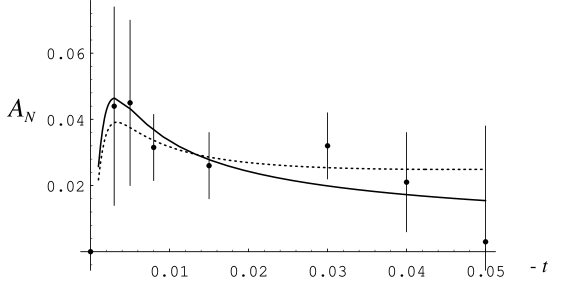
Figure 1: The data points are from Fermilab E704 [48]. The solid curve is the best fit with the hadronic amplitude $\phi_{5}$ constrained to be in phase with hadronic $\phi_{+}$ ; the dotted curve is the best fit without this constraint.

The errors are unfortunately too large to allow an unambiguous theoretical interpretation, but let us now briefly recall what can one learn from it. From the formulae in Section 2, $A_{N}$ is given by the expression (this is identical to the expression for the final state polarization parameter $P$)

$$A_{N}={{\mathop{\mathrm{Im}}\{(2\phi_{+}+2e^{i\delta}\phi_{+}^{\rm em}+\phi_{2})^{\ast}\,(\phi_{5}+e^{i\delta}\phi_{5}^{\rm em})\}}\over{|\phi_{+}+e^{i\delta}\phi_{+}^{\rm em}|^{2}+|\phi_{-}|^{2}+\frac{1}{2}|\phi_{2}|^{2}+2|\phi_{5}+e^{i\delta}\phi_{5}^{\rm em}|^{2}}}\,\,,$$ (27)

for not too large values of $-t$, such that the amplitude $\phi_{4}=\langle+-|\phi|-+\rangle$ may be ignored because of the kinematical factor $(-t)$ occuring in this double helicity-flip amplitude.

In the one-photon exchange approximation $\phi_{+}^{\rm em}$ and $\phi_{5}^{\rm em}$ are real and have well established expressions Eq. (2), so in order to make a theoretical prediction using Eq. (27), one needs to know the hadronic amplitudes $\phi_{+},\phi_{-},\phi_{2}$ and $\phi_{5}$. The imaginary part of the largest one, $\phi_{+}$, is related at $t=0$ to the total cross section $\sigma_{\rm tot}$ and the interference between $\phi_{5}^{\rm em}$ and $\phi_{+}$ is most prominent when $t=t_{c}$, where $t_{c}=-8\pi\alpha/\sigma_{\rm tot}$.

The explicit expression can be obtained by substituting the expressions from Section 2 into Eq. (27):

$$\frac{m\,A_{N}}{\sqrt{-t}}\,\frac{16\pi}{\sigma_{\rm tot}^{2}}\,\frac{d\sigma}{dt}\,e^{-Bt} = \left[\kappa\left(1-\delta\rho+\mathop{\mathrm{Im}}r_{2}-\delta\mathop{\mathrm{Re}}r_{2}\right)-2\,(\mathop{\mathrm{Im}}r_{5}-\delta\mathop{\mathrm{Re}}r_{5})\right]\frac{t_{c}}{t}$$

$$-2(1+\mathop{\mathrm{Im}}r_{2})\mathop{\mathrm{Re}}r_{5}+2(\rho+\mathop{\mathrm{Re}}r_{2})\mathop{\mathrm{Im}}r_{5},$$

$$\frac{16\pi}{\sigma_{\rm tot}^{2}}\,\frac{d\sigma}{dt}\,e^{-Bt} = \left(\frac{t_{c}}{t}\right)^{2}-2(\rho+\delta)\frac{t_{c}}{t}+\,(1+\rho^{2})(1+\beta^{2})\,,$$ (28)

where $\beta$ is defined in Eq. (2). The asymmetry for the CNI region can thus be expressed [49] as a quotient of a linear expression in $t_{c}/t$ in the numerator and a quadratic expression for $t_{c}/t$ in the denominator, neglecting terms of order $t$.

The Coulomb phase $\delta$ is small, about 0.02 in the CNI region, smaller at larger $|t|$. It has a slight effect on the position of the maximum in $A_{N}$:

$$\frac{t_{\mathrm{m}ax}}{t_{c}}=\sqrt{3}+\frac{8}{\kappa}(\rho\mathop{\mathrm{Im}}r_{5}-\mathop{\mathrm{Re}}r_{5})-(\rho+\delta)\,,$$ (29)

in the approximation where small quantities are kept to first order, but it enters the numerator multiplied by small amplitudes and so can be neglected for $pp$ scattering. The height of the peak is mainly sensitive to the unknown quantities $\mathop{\mathrm{Im}}r_{2}$ and $\mathop{\mathrm{Im}}r_{5}$, while the shape depends mainly on $\mathop{\mathrm{Re}}r_{5}$. For example, an $\mathop{\mathrm{Im}}r_{5}$ value of $\pm 0.1$ modifies the maximum of $A_{N}$ by about 11%.

There are two fits to the E704 data allowing a non-zero $r_{5}$ shown in Fig.1 [7]; the other $r_{i}$’s are set to zero. The solid curve is the best fit subject to the constraint that $\phi_{5}$ is in phase with $\phi_{+}$. The arguments in Section 2 show that if $\phi_{+}$ and $\phi_{5}$ have the same asymptotic behavior they will have the same phase; in that case the best fit is $|r_{5}|=0.0\pm 0.16$. Fitting without that constraint yields the dotted curve, which corresponds $|r_{5}|=0.2\pm 0.3$ with a relative phase angle to $\phi_{+}$ of $0.15\pm 0.27$ radians. Note the large uncertainties on these values. This is essentially the same as an earlier fit obtained in [50]. As emphasized in [7, 8], we see that a large value of $\mathop{\mathrm{Im}}r_{5}$ generates a very large uncertainty on $A_{\rm max}$, which can be of the order of 30% or more.

3.2 Energy dependence of the spin flip amplitudes from nucleon-nucleon scattering

In the small $t$ region we have some miscellaneous data on their magnitude and energy dependence. First, the transverse-spin total cross sections difference $\Delta\sigma_{\rm T}$ is related to $\mathop{\mathrm{Im}}r_{2}$ for $t=0$, according to $\mathop{\mathrm{Im}}r_{2}=-\Delta\sigma_{\rm T}/2\sigma_{\rm tot}$. From the limited ZGS data [51], we find that $\mathop{\mathrm{Im}}r_{2}$ decreases strongly in magnitude from $-6\%$ at $p_{L}=2\mbox{ GeV}/c$ to $-0.4\%$ at $p_{L}=6\mbox{ GeV}/c$. One can speculate whether for higher energy, it will remain negative and small or change sign and increase in magnitude. The charge exchange reaction $np\to pn$, can be also used to evaluate the modulus of $\phi_{2}$ which dominates the cross section near the forward direction. The analysis of the data [52], leads to the value $|r_{2}|=3.5\%$ at $p_{L}=25\mbox{ GeV}/c$ and $|r_{2}|=0.6\%$ at $p_{L}=270\mbox{ GeV}/c$, further evidence for a strong energy fall off of the $I=1$ exchange amplitude.

The longitudinal-spin total cross sections difference $\Delta\sigma_{\rm L}$ is related to $\mathop{\mathrm{Im}}r_{-}$ for $t=0$, according to $\mathop{\mathrm{Im}}r_{-}=\Delta\sigma_{\rm L}/2\sigma_{\rm tot}$. From the ZGS data [53], we find that $\mathop{\mathrm{Im}}r_{-}$ decreases strongly in magnitude, from $-10\%$ at $p_{L}=2\mbox{ GeV}/c$ to $-0.6\%$ at $p_{L}=12\mbox{ GeV}/c$. At higher energy, E704 has measured $\Delta\sigma_{\rm L}$ [54] for both $pp$ and $\bar{p}p$; their values imply that $\mathop{\mathrm{Im}}r_{-}$ has decreased below $10^{-3}$ for $pp$ and to about $10^{-3}$ (with a 100 % error) for $\bar{p}p$. These findings are consistent with the belief that $\mathop{\mathrm{Im}}\phi_{-}$ vanishes as $s\to\infty$.

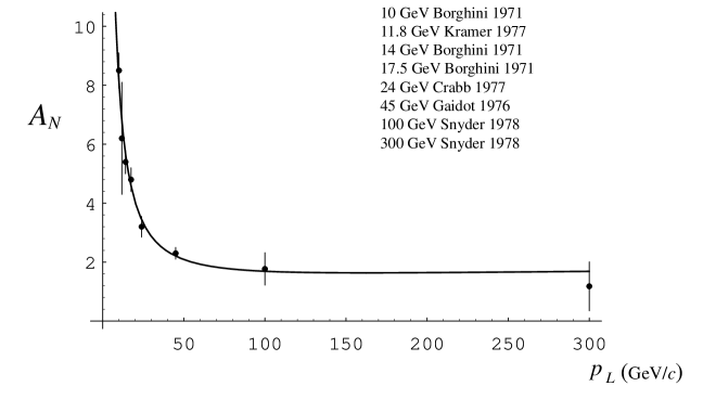
Figure 2: $A_{N}=P$ in percent as a function of lab momentum $p_{L}$ at $t=-0.15\ GeV^{2}$

Away from the forward direction and the CNI region, the data indicate that $A_{N}$ in $pp$ elastic scattering is falling very fast with energy. This has sometimes led to the conclusion that the helicity-flip amplitude $\phi_{5}$ would vanish as a power of $s$ as $s\to\infty$ [55]. In order to investigate this, we have taken a collection of data from various experiments which measure $P=A_{N}$ at different energies, all for $t=-0.15\mbox{ GeV}^{2}$ (or interpolated from nearby values), the smallest $|t|$ for which there is sufficient data to do this [56]. We have tried a fit suggested by Regge poles, namely $P=a+b/\sqrt{p_{L}}+c/p_{L}$ [7]. This is shown in Fig. 2 and the relevant result is that $a=0.023\pm 0.012$. It is not very well determined: it is consistent with pure CNI, which is approximately 0.01 at this value of $t$ and $p_{L}\approx 300\mbox{ GeV}/c$. At the same time it is consistent with a very large hadronic helicity-flip amplitude: the calculated value of $A_{N}$ with $\mathop{\mathrm{Im}}r_{5}=-0.6$ and $\mathop{\mathrm{Re}}r_{5}=-.015$ (so that $\phi_{5}$ is in phase with $\phi_{1}$) approximates the fit very well for $p_{L}$ above $200\ \mbox{GeV/c }$. Because of the phase energy relation discussed in Section 2, these data are consistent with a large helicity-flip pomeron coupling. The real and imaginary parts of $r_{5}$ cannot be separately determined from the measurement of $A_{N}$ at this one value of $t$ , but they could both be determined by measuring the $t$-dependence at RHIC because the deviation from the pure CNI shape is extremely sensitive to $\mathop{\mathrm{Re}}r_{5}$.

3.3 Iso-scalar part of the helicity-flip from $\pi^{\pm}p$ scattering

Detailed Regge fits were made to spin dependent measurements in the 1970’s [57, 58, 59, 60]. At the low energies at which those measurements were made, there were quite large asymmetries observed. It was found that these were mainly due to the low-lying Regge trajectories and were not very sensitive to the pomeron couplings. The parameters that were found do predict a very small ($<10\%$) ratio of the flip to non-flip residues for the pomeron, but the parameters are uncertain because of this insensitivity of the fits.

Polarization in $\pi p$ elastic scattering at high energy is mostly due to interference of the pomeron non-flip amplitude with the helicity-flip part of the $\rho$-Reggeon. As a consequence, the polarization has different signs and is nearly symmetric in $\pi^{\pm}p$ scattering. It decreases with energy as

$$A_{N}^{\pi p}(s,t)\propto\left(\frac{s}{s_{0}}\right)^{\alpha_{\rho}(t)-\alpha_{IP}(t)}\ ,$$ (30)

where $\alpha_{\rho}(t)\approx 0.5+0.9\ t$ and $\alpha_{IP}(t)\approx 1.1+0.25\ t$. The polarization has a double-zero behavior at $t\approx-0.6\mbox{ GeV}^{2}$, which is correlated to the change of sign of $\alpha_{\rho}(t)$ at this point; see Fig. 3. This effect can be understood as a result of destructive interference with the $\rho\otimes IP$ cut. An alternative explanation involves the wrong signature nonsense zero [58] (zeros in the residue and in the signature factor of the $\rho$-reggeon).

At very high energies this part of the polarization vanishes, and one can hope to detect an energy-independent contribution of the pomeron. Unfortunately, available data are not sufficiently precise yet. One can eliminate the large background from the $\rho\otimes IP$ contribution by adding the data on polarization in $\pi^{\pm}p$ elastic scattering,

$$\Sigma_{\pi p}(s,t)=\delta_{+}(s,t)\ \ A_{N}^{\pi^{+}p}(s,t)+\delta_{-}(s,t)\ \ A_{N}^{\pi^{-}p}(s,t)\ ,$$ (31)

where

$$\delta_{\pm}(s,t)=\frac{2\ \sigma^{\pi^{\pm}p}_{\rm el}(s,t)}{\sigma^{\pi^{+}p}_{\rm el}(s,t)+\sigma^{\pi^{-}p}_{\rm el}(s,t)}\ ,$$ (32)

and

$$\sigma^{\pi^{\pm}p}_{\rm el}(s,t)\equiv\frac{d\sigma^{\pi^{\pm}p}_{\rm el}(s,t)}{dt}\approx\frac{\sigma^{\pi^{\pm}p}_{\rm tot}(s)^{2}}{16\pi}\ \exp\left(B_{\rm el}^{\pi^{\pm}p}t\right)\ .$$ (33)

Therefore, Eq. (32) can be rewritten as,

$$\delta_{+}(s,t) = \frac{2\ \gamma(s,t)}{1+\gamma(s,t)}\ ,$$

$$\delta_{-}(s,t) = \frac{2}{1+\gamma(s,t)}\ ,$$ (34)

where

$$\gamma(s,t)=\left(\frac{\sigma^{\pi^{+}p}_{\rm tot}}{\sigma^{\pi^{-}p}_{\rm tot}}\right)^{2}\ e^{-\Delta B\,t}.$$ (35)

The difference between the elastic slopes $\Delta B\equiv B^{\pi^{-}p}_{el}-B^{\pi^{+}p}_{el}$ is related to the position of the cross-over point $t_{0}\approx-0.15\mbox{ GeV}^{2}$, which is nearly energy independent [61] in this energy range since

$$\Delta B(s)=\frac{2}{|t_{0}|}\ln\left(\frac{\sigma^{\pi^{-}p}_{\rm tot}(s)}{\sigma^{\pi^{+}p}_{\rm tot}(s)}\right).$$ (36)

To find $\delta_{\pm}(s,t)$ we fit the data on $\sigma^{\pi^{\pm}p}_{\rm tot}(s)$ [62] with the expression

$$\sigma^{\pi^{\pm}p}_{\rm tot}(s)=\sigma_{IP}\ \left(\frac{s}{s_{0}}\right)^{\alpha_{IP}(0)-1}+\sigma_{f}\ \left(\frac{s}{s_{0}}\right)^{\alpha_{f}(0)-1}\mp\sigma_{\rho}\ \left(\frac{s}{s_{0}}\right)^{\alpha_{\rho}(0)-1}.$$ (37)

We fixed $\alpha_{IP}(0)=1.1$, $\alpha_{f}(0)=\alpha_{\rho}(0)=0.5$, $s_{0}=1\,\mbox{GeV}^{2}$ and found $\sigma_{IP}=12.4\pm 0.03\mbox{ mb},\ \sigma_{f}=40.8\pm 0.26\mbox{ mb},\ \sigma_{\rho}=5.1\pm 0.07\mbox{ mb}$.

Due to the cancellation of the isovector terms in Eq. (31) $\Sigma_{\pi p}(s,t)$ is dominated by the interference of the pomeron with the leading isoscalar reggeons. In $\pi p$ scattering this can only involve $f$-reggeon interference.

Since the main part of the polarization cancels in the sum, the data have to have sufficiently high statistics in order to use Eq. (31). This is why we could only use the low-energy data at momenta $p_{L}=6-14\mbox{ GeV}/c$, depicted in Fig. 3.

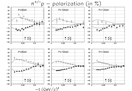
Figure 3: Polarization in $\pi p$ elastic scattering in the energy range $6-14\ GeV$. The data points are from [63]-[65]. The curves show our fit with the parameterization Eq. (39) - Eq. (40).

We performed a fit of $A_{N}^{\pi^{\pm}p}(s,t)$ with the parameterization

$$A_{N}^{\pi^{\pm}}(s,t)=\frac{\Sigma_{\pi p}(s,t)\pm\Delta_{\pi p}(s,t)}{2\ \delta_{\pm}(s,t)},$$ (38)

where

$$\Delta_{\pi p}(s,t)=\frac{\sqrt{|t|}}{m_{N}}\ e^{a_{1}t}\,(a_{2}+a_{3}t)(t-a_{4})^{2}\ K(s)\,\left(\frac{s}{s_{0}}\right)^{\alpha_{R}(t)-\alpha_{IP}(t)}\ ,$$ (39)

and

$$\Sigma_{\pi p}(s,t)=\frac{\sqrt{|t|}}{m_{N}}\ e^{a_{1}t}\,(a_{5}+a_{6}t)\ K(s)\,\left(\frac{s}{s_{0}}\right)^{\alpha_{R}(t)-\alpha_{IP}(t)},$$ (40)

Here $t$ is in $(\mbox{GeV}/c)^{2}$. We use the same energy dependence for $\Sigma_{\pi p}(s,t)$ and $\Delta_{\pi p}(s,t)$ assuming that $\alpha_{R}(t)=\alpha_{\rho}(t)=\alpha_{f}(t)$. The factor

$$K^{-1}(s)=1+2\ \frac{\sigma_{f}}{\sigma_{IP}}\,\left(\frac{s}{s_{0}}\right)^{\alpha_{R}(t)-\alpha_{IP}(t)}+\left\{\frac{\sigma_{f}}{{\rm sin}\left[\frac{\pi}{2}\,\alpha_{f}(0)\right]\sigma_{IP}}\,\left(\frac{s}{s_{0}}\right)^{\alpha_{R}(t)-\alpha_{IP}(t)}\right\}^{2}$$ (41)

takes into account the contribution of the $f$-reggeon to the differential cross section. The parameter $a_{1}$ corresponds to the difference between the slopes of the pomeron and $f$-reggeon amplitudes. The factor $(t-a_{6})^{2}$ is introduced to reproduce the double-zero behavior of the polarization clearly seen in data [63]-[65]. It is usually related to presence of an additional zero in the $\rho$-reggeon residue which is dictated by duality at $\alpha_{\rho}=0$ [58].

The result of the fit is shown by the solid curves in Fig. 3, and the values of the parameters $a_{i}$ are collected in Table 2.

$a_{1}$	$a_{2}$	$a_{3}$	$a_{4}$	$a_{5}$	$a_{6}$
$2.5$	$12.5$	$68.5$	$0.7$	$0.77$	$2.33$
$\pm.2$	$\pm 1.0$	$\pm 8.2$	$0.01$	$\pm 0.13$	$0.59$

Table 2: Fitted values of the parameters $a_{i}$

The ratio of the helicity-flip to non-flip isosinglet amplitudes can be extracted from $\Sigma_{\pi p}(s,t)$,

$$r_{f}(t)-r_{IP}(t)={1\over 4}\,e^{a_{1}t}\,(a_{5}+a_{6}t)\frac{\sigma_{IP}}{\sigma_{f}}\tan\left(\frac{\pi\alpha_{f}(t)}{2}\right).$$ (42)

Here $r_{IP}\sqrt{|t|/m^{2}}$ and $r_{f}\sqrt{|t|/m^{2}}$ denote the ratio of the helicity-flip to non-flip amplitude corresponding to $IP$ and $f$ exchange, respectively. We assume here that the helicity-flip and non-flip amplitudes have the same phase which corresponds to dominance of Regge poles. We neglect the real part of the pomeron amplitude. If we assume factorization, then for $pp$ scattering, asymptotically, $\mathop{\mathrm{Im}}r_{5}(s,t)\approx r_{IP}(t)$.

Thus, the combination Eq. (42) of spin-flip to non-flip ratios for iso-singlet amplitudes, which is quite difficult to measure directly, are fixed by this analysis with a good accuracy.

$$r_{f}(0)-r_{IP}(0)=0.06\pm 0.01\ .$$ (43)

Unfortunately, without further information regarding $r_{f}$, this does not restrict $r_{IP}$. The approximation of $f$-dominance of the pomeron yields $r_{IP}=r_{f}$, which obviously contradicts Eq. (43). The pion exchange model in Section 5.2 predicts values for both $r_{IP}$ and $r_{f}$ which are in pretty good agreement with Eq. (43). The Regge fits of [58] use $r_{f}=0$. This would give $r_{IP}=-0.06$, a very interesting value as we will see in Section 5. However, this should probably be disregarded because the fits of [58] also set the pomeron helicity-flip coupling to zero. The fits of [59] give, assuming exchange degeneracy and using the $\omega$ Regge residues, $r_{f}=0.95/10.6\approx 0.09$ and so, from Eq. (43), $r_{IP}=0.03$. Since this result requires some theory that is not tested to this precision, this can be taken as provisional but suggestive.

Another source of information on the isoscalar exchanges is $pA$ scattering. This requires special attention which we leave to another occasion.

4 Model-independent bounds and the energy dependence of helicity-flip

The magnitude of $r_{5}$ depends on the scale $1/m$ chosen in Eq. (2), where $m$ denotes the nucleon mass. This scale has been used conventionally for many years; it was probably chosen in analogy to the form of the one-photon exchange helicity-flip amplitude. It is not at all certain that this is the appropriate scale for the scattering of strongly-interacting particles with structure. It might be more natural for the scale to be set by the slope of the diffraction peak; i.e. the effective radius of the proton $R(s)=\sqrt{2B(s)}$, (we take this to be the definition of the quantity $R(s)$, see Eq. (54) and Eq. (56) below.) Since this is a good deal larger than $1/m$, the “natural” size of $r_{5}$ might be expected to be larger than 1. Furthermore, it might very well be expected to increase slowly with energy, corresponding to the growth in the effective radius of the proton. This, of course, flies in the face of conventional wisdom; see the discussion of Section 3.

It is natural to investigate if there is a theoretical argument that $r_{5}\rightarrow 0$ as $s\rightarrow\infty$. We begin by remarking that for the pure Coulomb amplitudes this is not true, so we ask if there is something different about the hadronic amplitudes. One obvious difference is that experimentally $\phi_{+}$ grows faster than $s$, and presumably will eventually grow as $s\ln^{2}{s}$, the maximum rate allowed by the Froissart-Martin bound [30]. Let us see what the same arguments used to derive that bound yield when applied to $\phi_{5}$. The partial wave expansion for $\phi_{5}$ is [66]

$$\phi_{5}(s,t) = \sum_{J}(2J+1)f_{J}^{5}(s)d_{10}^{J}(\theta)$$ (44)

$$= \frac{\sin{\theta}}{2}\sum_{J}(2J+1)\sqrt{\frac{J+1}{J}}f_{J}^{5}(s)P_{J-1}^{(1,1)}(\cos{\theta}),$$

where $t=-2k^{2}(1-\cos{\theta})$ and $P_{J}^{(l,m)}(\cos{\theta})$ denotes the Jacobi polynomial in $\cos{\theta}$ [67]. From this one finds that

$$\hat{\phi_{5}}(s,0)={m\over\sqrt{s}}\sum_{J}(2J+1)\sqrt{\frac{J+1}{J}}f_{J}^{5}(s)P_{J-1}^{(1,1)}(1),$$ (45)

where $\hat{\phi_{5}}=m/\sqrt{-t}\ \phi_{5}$. Partial wave unitarity requires that [68]

$$2|f_{5}^{J}(s)|^{2}\leq\mathop{\mathrm{Im}}{f_{+}^{J}(s)}(1-\mathop{\mathrm{Im}}{f_{+}^{J}(s)})\leq 1/4.$$ (46)

If we assume that this bound is saturated out to some $L_{\rm max}(s)\sim kR(s)$, where $k\approx\sqrt{s}/2$ is the cm momentum, then using $P_{J-1}^{(1,1)}(1)=J$ (to be compared with $P_{J}(1)=1$ for the Legendre polynomials) we find that for $s\rightarrow\infty$, $\hat{\phi_{5}}(s,0)$ goes as $m\,s\,R^{3}(s)$ while $\phi_{+}$ goes as $s\,R^{2}(s)$, and so the natural scale for $\hat{\phi_{5}}(s,0)$ is $R(s)$, not $1/m$. This means that unitarity and other general principles allow $r_{5}$ to grow with energy; if the Froissart bound is saturated $L_{\rm max}\sim\sqrt{s}\ln{s}$ and $r_{5}\sim\ln{s}$ is allowed. Note that if $L_{\rm max}\sim\sqrt{s\ln{s}}$ then $\sigma_{\rm tot}$ will grow only as $\ln{s}$ as favored by Block et al [29]; in that case, $r_{5}\sim\ln^{1/2}{s}$ is allowed.

The above argument assumed the same $L_{\rm max}$ for $\phi_{+}$ and $\phi_{5}$. This can, in fact, be proved as follows: one can bound $P_{J}^{(1,1)}$ from below, parallel to Martin’s argument for $P_{l}$, the Legendre polynomial, in the unphysical region $|\cos{\theta}|>1$. One then applies the same reasoning as he used for $\phi_{+}$ to $\phi_{5}$. The representation

$$P_{J-1}^{(1,1)}(x)=\frac{2J}{\pi}\int_{0}^{\pi}d\phi\ (x+\sqrt{x^{2}-1}\cos{\phi})^{J-1}\sin^{2}{\phi}$$ (47)

allows one to show that $P_{J-1}^{(1,1)}(x)\sim x^{J}/\sqrt{J}$ as $J\rightarrow\infty$ for $x>1$. This is the same as the asymptotic behavior obtained for the $P_{l}(x)$ by Martin, and so polynomial boundedness implies the same $L_{\rm max}$ for $\phi_{5}$ and $\phi_{+}$.

Notice that the same arguments applied to the double-flip amplitudes $\phi_{4}(s,t)$ or $d\phi_{2}(s,t)/dt|_{t=0}$ will yield a natural scale of $R^{2}(s)$ and, correspondingly, a possible growth with energy as fast as $\ln^{4}{s}$.

One can easily see that $\phi_{5}$ can grow faster with $s$ than $\phi_{+}$ without violating unitarity because of the factor of $\sqrt{-t}$. It is, naturally, an interesting question to determine to what degree the helicity-flip amplitudes saturate unitarity, even at energies where the Froissart bound is not saturated. Techniques using unitarity and partial wave expansions have been used in the past at low energy to obtain bounds on the helicity-flip amplitude in terms of $\sigma_{\rm tot}$, $\sigma_{\rm el}$ and $B$ [69, 70, 71]; these bounds are comparable in size to $mR/2$, i.e. $r_{5}$ is found to lie between 2 and 3.

We can make the discussion of unitarity more quantitative by transforming the scattering amplitudes to the impact parameter representation. To keep the discussion as simple as we can, let us do this for scattering of a proton on a spin 0 target; as a $2\times 2$ matrix, the scattering amplitude has the form

$$\frac{2\pi}{\sqrt{s}}f(\vec{k^{\prime}},\vec{k})=g_{1}(s,q)+\vec{\sigma}\cdot\frac{\vec{k}\times\vec{k^{\prime}}}{|\vec{k}\times\vec{k^{\prime}}|}g_{2}(s,q),$$ (48)

where $\vec{q}=\vec{k^{\prime}}-\vec{k}$ , $q=|\vec{q}|$ and $q^{2}=-t$ for elastic scattering.

The two-dimensional Fourier transforms of these into impact parameter space yields the profile functions $\tilde{g_{1}(b,s)}$ and $\tilde{g_{2}(b,s)}$:

$$\frac{2\pi}{\sqrt{s}}\int{\frac{d^{2}\vec{q}}{2\pi}\,e^{\imath\,\vec{q}\cdot\vec{b}}f(\vec{k^{\prime}},\vec{k})}=\tilde{g_{1}}(b,s)+\imath\,\vec{\sigma}\cdot\frac{\vec{b}\times\vec{k}}{bk}\tilde{g_{2}}(b,s),$$ (49)

where

$$\tilde{g_{1}}(b,s) = \int{\frac{d^{2}\vec{q}}{2\pi}\,e^{\imath\,\vec{q}\cdot\vec{b}}}g_{1}(s,q),$$

$$\tilde{g_{2}}(b,s) = i\int{\frac{d^{2}\vec{q}}{2\pi}\,e^{\imath\,\vec{q}\cdot\vec{b}}\,\hat{b}\cdot\hat{q}}\,g_{2}(s,q).$$ (50)

With this normalization

$$\sigma_{\rm tot}(s)=4\pi\int{b\ db\mathop{\mathrm{Im}}{\tilde{g_{1}}(b,s)}},$$ (51)

and unitarity imposes, for each value of $b$, the condition

$$2\mathop{\mathrm{Im}}{\tilde{g_{1}}}(b,s)\geq|\tilde{g_{1}}(b,s)|^{2}+|\tilde{g_{2}}(b,s)|^{2}.$$ (52)

(This equation is, in general, only approximate in $b$ space, but it can be derived from the analogous partial wave inequality [68] if only the elastic scattering amplitudes are sufficiently peaked in $t$.) The bounds discussed earlier correspond to a uniform distribution in $b$ for both amplitudes for $b\leq R=L_{\rm max}/k$. If this $b$-distribution is translated into the $t$-dependence of the amplitudes near $t=0$ it implies that the slope of $g_{2}/\sqrt{-t}$ is less than the slope $B=L_{\rm max}^{2}/2k^{2}$ of $g_{1}$; in fact it is $3B/5$.

A more conventional assumption is that the slopes of $g_{1}$ and $g_{2}/\sqrt{-t}$ are the same. If, in fact, $g_{2}(s,q)=\lambda\ (q/m)\,g_{1}(s,q)$, with $\lambda$ independent of $t$ then

$$\tilde{g_{2}}(b,s)=\frac{\lambda}{m}\frac{d\tilde{g_{1}}(b,s)}{db}.$$ (53)

This is true in the optical model or in any other model where the potential shape or matter distribution is the same for spin-orbit force as for the purely central force. Then $\tilde{g}(s,b)$ will be more peripheral than for the bound just discussed. It has nothing intrinsically to do with unitarity or saturation of the Froissart bound, and it is clearly interesting to determine whether it is true or not.

The unitarity condition Eq. (52) imposes a bound on $|\lambda|$, and the closer $\tilde{g_{1}}(b,s)$ is to saturating unitarity, the stronger this bound will be. Approximating the $t$-dependence of the amplitude by a logarithmically shrinking diffraction peak and neglecting its real part gives

$$\tilde{g_{1}}(b,s)=\frac{i\,\sigma(s)}{2\pi R^{2}(s)}\,{\rm exp}\left[-\frac{b^{2}}{R^{2}(s)}\right]\ ,$$ (54)

and

$$\tilde{g_{2}}(b,s)=-\frac{2\ ib\,\lambda\,\sigma(s)}{2\pi mR^{4}(s)}\,{\rm exp}\left[-\frac{b^{2}}{R^{2}(s)}\right]\ ,$$ (55)

where here and in the rest of this section the energy dependent Regge radius of interaction is

$$R^{2}(s)=R_{0}^{2}+4\alpha^{\prime}_{IP}\,{\rm ln}\left({s\over s_{0}}\right).$$ (56)

With this form for the amplitudes $\sigma(s)=\sigma_{\rm tot}(s)$ via Eq. (51). This will change at the next stage of the calculation. Here one finds, numerically, over a wide range of values of $\sigma(s)/2\pi R^{2}(s)\leq 1$ that

$$|\lambda|\leq mR\sqrt{\frac{2\pi R^{2}(s)}{\sigma(s)}}$$ (57)

is required in order to satisfy Eq. (52).

If $\sigma(s)$ grows faster than $R^{2}(s)$ with $s$ as $s\to\infty$, say as $s^{\Delta_{IP}}$ [31], then the amplitude Eq. (54) will eventually violate the unitarity condition Eq. (52) and the form must be modified. It is well-known that the total $pp$ cross section at available energy is still far below the Froissart-Martin bound; however, the bound Eq. (52) is already saturated at small impact parameters, even ignoring the helicity-flip piece [34, 72]. In principle, unitarity is restored after all the Regge cuts generated by multi-pomeron exchanges are added [35]. A standard way of unitarization of the non-flip part of the pole amplitude [58] is eikonalization; however, the presence of the helicity-flip component may lead to problems with unitarity. Indeed, an even number of repeating helicity-flip amplitudes contribute to the non-flip part, but all of them grow as a power of energy and have the same sign. Therefore, eikonalization of the helicity-flip amplitude alone does not save unitarity, which can be restored only after the absorptive corrections due to initial/final state spin non-flip interactions are included. The resulting profile function reads,

$$\tilde{g_{1}}^{eik}(b,s)=1-{\rm exp}[i\,\tilde{g_{1}}(b,s)]+\left\{1-{\rm cosh}\left[\frac{2\,i\,\lambda\,b}{m\,R^{2}(s)}\,\tilde{g_{1}}(b,s)\right]\right\}\,{\rm exp}[i\,\tilde{g_{1}}(b,s)].$$ (58)

The first two terms on the r.h.s. of this equation correspond to eikonalization of the non-flip part of Eq. (48). They obey the unitarity bound at any $s$ and $b$. In the extreme asymptotic region where $\sigma(s)$ in Eq. (54) and Eq. (55) is much greater than $R^{2}(s)$ then the $b$-dependence has the form of a “black disk”, i.e. $\tilde{g_{1}}^{eik}(b,s)=1$ at $b<\widetilde{R}(s)$ and vanishes at $b>\widetilde{R}$, where [35],

$$\widetilde{R}^{2}=\Delta_{IP}\,{\rm ln}\left({s\over s_{0}}\right)\,R^{2}(s)\ ,$$ (59)

if $\sigma(s)\sim(s/s_{0})^{\Delta_{IP}}$. Likewise,

$$\tilde{g_{2}}^{eik}=-{\rm sinh}\left[\frac{2\,i\,\lambda\,b}{m\,R^{2}(s)}\,\tilde{g_{1}}(b,s)\right]\,{\rm exp}[i\,\tilde{g_{1}}(b,s)].$$ (60)

Problems with unitarity at $b<\widetilde{R}(s)$ may arise from the last term in Eq. (58). The condition Eq. (52) is satisfied if

$$|\mathop{\mathrm{Re}}\lambda|<\frac{m\,R^{2}(s)}{2\,b}.$$ (61)

The minimal bound corresponds to a maximal $b=\widetilde{R}$, and $s\to\infty$,

$$|\mathop{\mathrm{Re}}\lambda|<m\,\left(\frac{\alpha^{\prime}_{IP}}{\Delta_{IP}}\right)^{1\over 2}.$$ (62)

For reasonable values of $\alpha_{IP}^{\prime}$ and $\Delta_{IP}$ we conclude that $|\mathop{\mathrm{Re}}\lambda|<1.6$. This is not a severe restriction, and is valid only in the extreme asymptotic limit, beyond the RHIC range; numerical calculations give a much larger bound, of order $mR$ at RHIC energies.

Note that $\lambda$ is renormalized by the eikonalization process; the result, $\lambda^{eik}(s)$ can be calculated numerically from

$$\lambda^{eik}(s)=\frac{m\int{db\ b^{2}\tilde{g_{2}}^{eik}(b,s)}}{2\int{db\ b\,\tilde{g_{1}}^{eik}(b,s)}}.$$ (63)

Likewise, the total cross section will be modified from the input values $\sigma(s)$ and is given by

$$\sigma_{\rm tot}(s)=4\pi\int{b\ db\mathop{\mathrm{Im}}\tilde{g_{1}}^{eik}(b)}.$$ (64)

These last two equations will have to be used for comparison with data.

5 Models for the pomeron helicity-flip

An early attempt to understand the spin structure of the pomeron coupling was made by Landshoff and Polkinghorne [73]. This model preceded the formulation of QCD, but used some of its features in a model they called the dual quark-parton model. They argued that the $t$-dependence of the pomeron coupling was determined by the electromagnetic form factors of the proton and neutron. This led to the conclusion that the helicity-flip coupling is given by the isoscalar anomalous magnetic moment of the nucleons; in our notation $r_{5}=(\mu_{p}-1+\mu_{n})/2=-0.06$. This relation has subsequently been obtained or conjectured independently in a variety of models based on QCD. The result is, however, model-dependent as we will see.

5.1 Perturbative QCD

There is a widespread prejudice that the perturbative pomeron does not flip helicity. It is true that the perturbative pomeron couples to a hadron through two $t$-channel gluons, and that the quark-gluon vertex $\bar{u}_{q}\gamma_{\mu}u_{q}$ conserves helicity. However, one cannot jump to the conclusion that the same is true for a proton. In QED the fundamental vertex has the same form but radiative corrections induce helicity-flip via an anomalous magnetic moment. Ryskin [74] evaluated the pomeron helicity-flip coupling by analogy to the isoscalar anomalous magnetic moment of the nucleon. Applying this analogy to the quark gluon vertex he found the anomalous color magnetic moment of the quark. Thus the quark-gluon vertex does not conserve helicity and one can calculate the helicity-flip part of the pomeron-proton vertex. Using the two-gluon model for the pomeron and the nonrelativistic constituent quark model for the nucleon he found [74]

$$\mathop{\mathrm{Im}}r_{5}=0.13,$$ (65)

independent of energy. In the above one needs to introduce an effective gluon mass and if one takes a large effective gluon mass, $m_{g}\approx 0.75\mbox{ GeV}$, this estimate is substantially reduced. A need for a large gluon mass follows from lattice QCD calculations [75] and the smallness of the triple-pomeron coupling [76].

The spin-flip part of the three-gluon odderon was also estimated in [74] and the helicity-flip component was found to be nearly the same as for the pomeron. If this is so then the odderon-pomeron interference contribution to $A_{N}$ vanishes. See Eq. (2) and Table 3 in Section 6.

An alternative approach is to note that helicity is defined relative to the direction of the proton momentum, while the quark momenta are oriented differently. Therefore, the proton helicity may be different from the sum of the quark helicities [6]. The results of perturbative QCD calculations show that the helicity-flip amplitude in elastic proton scattering very much correlates with the quark wave function of the proton. Spin effects turn out to cancel out if the spatial distribution of the constituent quarks in the proton is symmetric [6, 77]. However, if a quark configuration containing a compact diquark ($ud$) dominates the proton wave function, the pomeron helicity-flip part is nonzero. The more the proton wave function is asymmetric, i.e. the smaller the diquark is, the larger is $\mathop{\mathrm{Im}}r_{5}$ [6, 77]. Its value in the CNI region of transverse momentum ranges from $-0.05$ to $-0.1$ and even to $-0.15$ for the diquark diameters $0.5$, $0.3$ and $0.2\,{\rm fm}$, respectively. The commonly accepted diquark size is $0.3-0.4\ {\rm fm}$; therefore, we conclude that $|\mathop{\mathrm{Im}}r_{5}|$ does not exceed $10\%$.

Note that there is a principal difference in sensitivity to the proton wave function between the helicity-flip and the non-flip components of the pomeron. The former probes the shortest interquark distances in the proton (diquark), but the latter is sensitive to the largest quark separation (due to color screening). Correspondingly, the virtuality of the gluons in the pomeron is higher in the helicity-flip component since these gluons must resolve the diquark structure. This fact may be considered as a justification for perturbative calculations for the helicity-flip part, while their validity for the non-flip part is questionable.

High gluon virtuality in the helicity-flip pomeron leads to a steep energy dependence. A prominent experimental observation at HERA is that the steepness of growth with energy of the total virtual photoabsorption cross section correlates with the photon virtuality $Q^{2}$, i.e. with the $q\bar{q}$ separation in the hadronic fluctuation of the photon. Analyses of the data for the proton structure function $F_{2}(x,Q^{2})$ performed in [78] shows that for a quark separation of the order of the mean diquark diameter one should expect the energy dependence $\sim(s/s_{0})^{0.2}$. This should be compared with the well known energy dependence of the non-flip amplitude, $\sim(s/s_{0})^{0.1}$. Therefore if the perturbative QCD model is meaningful in this region we expect a negative $\mathop{\mathrm{Im}}r_{5}$ with energy dependence $(s/s_{0})^{0.1}$. This prediction can be tested in future polarization experiments at RHIC whose energy ranges from $s\approx 50\mbox{ GeV}^{2}$ (with a fixed target) up to $25\times 10^{4}\mbox{ GeV}^{2}$. $\mathop{\mathrm{Im}}r_{5}$ is expected to double its value in this interval.

Eventually this growth will cause the bound Eq. (62) to be violated. This occurs only at very high energy, well above the LHC energy, and so it is not important for our considerations. Nevertheless, it would be interesting to develop an eikonalization method that would lead to consistent unitary amplitudes. We believe the eikonalization procedure developed in [79] is the appropriate technique. When the elastic amplitude depends on transverse separation between partons, as it does here, the measured amplitude is the result of averaging over different transverse configurations:

$$\tilde{f}(b,s)=\langle\tilde{f}(b,s,\psi)\rangle_{\psi},$$ (66)

where $\psi$ characterizes the transverse configuration and the averaging is weighted by the probability to be in configuration $\psi$. Correspondingly, eikonalization has to be done first for a given configuration $\psi$ and only then averaged :

$$\tilde{f}^{eik}(b,s)=\langle\tilde{f}^{eik}(b,s,\psi)\rangle_{\psi}.$$ (67)

For a given partonic configuration $\psi$ the energy dependence of the helicity-flip and non-flip components must be the same since, as stated above, it depends only on the transverse separations. Therefore, restriction Eq. (62) applies except that the pomeron intercept depends on $\psi$ and unitarity is satisfied for each $\psi$. However, the weight factors are different for the helicity-flip and non-flip amplitudes and the averaging results in a higher effective intercept for the helicity-flip component. The detailed predictions of this procedure remain to be worked out.

5.2 Pion exchange model

A nucleon is known to have a pion cloud of large radius. Since the helicity-flip amplitude is proportional to impact parameter, it is natural that a substantial fraction comes from inelastic interaction of the projectile hadron with virtual peripheral pions. This contribution is related through the unitarity relation to a pomeron-nucleon vertex (in the elastic hadron-nucleon amplitude) shown in Fig. 4.

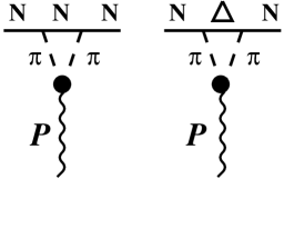
Figure 4: Pomeron coupling to a nucleon via two pion exchange.

It is known that the main contribution to the pion cloud comes from the virtual transitions $N\to\pi N$ and $N\to\pi\Delta$, which corresponds to the two graphs depicted in Fig. 4. This model for the pomeron-nucleon coupling was suggested in [80]. They predicted $\mathop{\mathrm{Im}}r_{5}\approx 0.016\,(\ln{s})^{3/2}$. This quite a steep energy dependence originates from the radius of the pion cloud which is assumed to be proportional to $\sqrt{\ln{s}}$. A more detailed analyses was undertaken in [81]. An interesting observation of this paper is a strong correlation of the value of $r_{5}$ with isospin in the $t$-channel. Namely, for an isoscalar exchange ($IP$, $f$-reggeon) the two graphs in Fig. 4 essentially cancel in the helicity-flip, but they add up in the non-flip amplitude. It is vice versa for an isovector exchange ($\rho$-reggeon). This conclusion is consistent with Regge phenomenological analyses of experimental data (see e.g. [82]).

In order to fix the parameters of the model a detailed analysis of data on inclusive nucleon ($pp\to p(n)X$) and $\Delta$ ($pp\to\Delta^{++}X$ and $\pi^{+}p\to\Delta^{++}X$) production was performed in [81]. These reactions correspond to the unitarity cut of the graphs in Fig. 4. The calculations in [81] led to a positive value of $\mathop{\mathrm{Im}}r_{5}=0.06$ for the pomeron (0.15 for the $f$-reggeon). This nonperturbative contribution has the opposite sign to what follows from perturbative calculations and may partially compensate it (see discussion in [6]).

5.3 Impact picture

An impact picture approach, which was derived several years ago [83, 84, 85], describes successfully $\bar{p}p$ and $pp$ elastic scattering up to ISR energies . It led to predictions at very high energy, so far in excellent agreement with the data from the CERN SPS collider and the FNAL Tevatron and others, which remain to be checked at the Large Hadron Collider under construction at CERN . The spin-independent amplitude reads at high energies

$$\phi_{+}^{impact}(s,t)=is\int^{\infty}_{0}J_{0}(b\sqrt{-t})(1-e^{-\Omega_{0}(s,b)})bdb~{},$$ (68)

where the opaqueness $\Omega_{0}$, which is assumed to factorize as $\Omega_{0}(s,b)=S_{0}(s)F(b^{2})$, is associated with the pomeron exchange. The energy dependence is given by the crossing symmetric function

$$S_{0}(s)=s^{c}/\ln^{c^{\prime}}{s}+u^{c}/\ln^{c^{\prime}}{u}~{},$$ (69)

which comes from the high energy behavior of quantum field theory. In $S_{0}(s)$ above, $u$ is the third Mandelstam variable and both $s$ and $u$ are expressed in $\mbox{GeV}^{2}$. Note that $S_{0}(s)$ is complex because $u$ is negative. The phenomenological analysis leads to the values of the two free parameters $c=0.167$, $c^{\prime}=0.748$ and the real part of $\phi_{+}^{impact}(s,t)$ results from the phase of $S_{0}(s)$. The $t$-dependence of $\phi_{+}^{impact}(s,t)$ is driven by $F(b^{2})$, which is related to the Fourier transform of the electromagnetic proton form factor and, as a result of a simple parametrization which can be found in [83], $F(b^{2})$ is fully determined in terms of only four additional parameters.

The spin structure of the model was also studied and it allows a rather good description of the polarization data, up to the highest available energy, i.e. $p_{L}=300\mbox{ GeV}/c$ [86]. At the RHIC energies, the spin dependent amplitude reads

$$\phi_{5}^{impact}(s,t)=is\int^{\infty}_{0}J_{1}(b\sqrt{-t})\Omega_{1}(s,b)e^{-\Omega_{0}(s,b)}bdb~{},$$ (70)

where $\Omega_{1}(s,b)$ is the spin dependent opaqueness, corresponding to the helicity-flip component of the pomeron. It also factorizes as $\Omega_{1}(s,b)=S_{1}(s)F_{s}(b^{2})$, where $S_{1}(s)$ is obtained from $S_{0}(s)$ and we have

$$S_{1}(s)={s^{c}\over\ln^{c^{\prime}}{s}}(c-c^{\prime}/\ln{s})+(s\rightarrow u)~{}.$$ (71)

$F_{s}(b^{2})$ is simply related to $F(b^{2})$ according to $F_{s}(b^{2})=b\omega(b^{2})F(b^{2})$, where $\omega(b^{2})$ is a smooth function which is not very precisely known. The important point is its value $\omega_{0}$ for very small $b$ and by fitting the data, it was found that $\omega_{0}=0.06\mbox{ GeV}$. This leads to a value $\mathop{\mathrm{Im}}r_{5}\approx-0.06$, if one assumes that the flip component of the pomeron is normalized at $t=0$, by the nucleon isoscalar magnetic moment [11]. This is at variance with the exact results one obtains in the impact picture, which are shown in Fig. 5 at two different energies. It is interesting to remark that $\mathop{\mathrm{Im}}r_{5}(t)$ increases with energy, in a way pretty much consistent with what was mentioned above in Section 4.

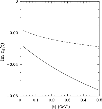
Figure 5: $\mathop{\mathrm{Im}}r_{5}(t)$ calculated in the impact picture for two energy values: $\sqrt{s}=50\mbox{ GeV}$ (dashed curve) and $\sqrt{s}=500\mbox{ GeV}$ (solid curve) .

6 $P$-independent determination of ${\bf\phi_{2}}$, ${\bf\phi_{-}}$, ${\bf\phi_{4}}$ and ${\bf\phi_{5}}$

In this section we would like to demonstrate that, in principle, by making use of both CNI and hadronic interference at small $t$ it is possible to determine all the spin dependent amplitudes at $t=0$ independent of knowledge of the beam polarization $P_{1}$ and $P_{2}$ provided only that they are stable and non-zero. This is very interesting, perhaps surprising, in its own right. If it proves to be practical, it would permit the use of elastic $pp$ scattering as a self-calibrating polarimeter. It is important to emphasize right at the beginning—we will not repeat this every time the issue occurs—that the method involves several ratios of very small quantities; the precision required to do this may be beyond the reach of practical experiment at this time. However, very little is known about the amplitudes now, and so we cannot evaluate this. Even if the complete process we describe cannot be carried through, much of what follows should be useful in constraining the amplitudes at small $t$.

The method requires the use of asymmetries with both longitudinal and transversely polarized beams; it will not work unless data are available with both configurations. Here we work only to order $\alpha$ and so only amplitudes that are large compared to the next order correction can be determined from the formulas given below. This could probably be improved upon if necessary; at the present, experiment will probably not be able to probe amplitudes below that size and so we have not pressed on in this direction. We assume that the polarized beams have the same degree of polarization $P$ in either configuration; since they are produced from the same initial configuration by rotation this is almost certainly true. For simplicity in writing we assume both beams to have the same polarization; this may very well not be true but it is trivial to correct the formulas for this.

We work with the experimentally measured asymmetries which are given by $PA_{N}$, $P^{2}A_{NN}$, etc. These will contain singular terms as $t\rightarrow 0$ coming from the interference between the one-photon exchange and the hadronic amplitudes. To order $\alpha$ the asymmetries $A_{NN},A_{SS}$ and $A_{LL}$ are singular as $1/t$ and $A_{N},A_{SL}$ are singular as $1/\sqrt{-t}$. So we write

$$\frac{m\sqrt{-t}}{\sigma_{\rm tot}}\,PA_{N}\,\frac{d\sigma}{dt} = -\alpha\,a_{N}+\frac{\sigma_{\rm tot}}{8\pi}\,b_{N}\,t+\ldots,$$

$$\frac{t}{\sigma_{\rm tot}}\,P^{2}A_{LL}\,\frac{d\sigma}{dt} = \alpha\,a_{LL}+\frac{\sigma_{\rm tot}}{8\pi}\,b_{LL}\,t+\ldots,$$

$$\frac{t}{\sigma_{\rm tot}}\,P^{2}A_{NN}\,\frac{d\sigma}{dt} = \alpha\,a_{NN}+\frac{\sigma_{\rm tot}}{8\pi}\,b_{NN}\,t+\ldots,$$

$$\frac{t}{\sigma_{\rm tot}}\,P^{2}A_{SS}\,\frac{d\sigma}{dt} = \alpha\,a_{SS}+\frac{\sigma_{\rm tot}}{8\pi}\,b_{SS}\,t+\ldots,$$

$$-\frac{m\sqrt{-t}}{\sigma_{\rm tot}}\,P^{2}A_{SL}\,\frac{d\sigma}{dt} = \alpha\,a_{SL}+\frac{\sigma_{\rm tot}}{8\pi}\,b_{SL}\,t+\ldots.$$ (72)

In the following table we give expressions for the various $a_{i}$, which we sometimes refer to as the enhanced pieces, and $b_{i}$ which we refer to as the hadronic piece. The $a_{i}$’s are linear in the hadronic amplitudes while the $b_{i}$ are bilinear. Here we omit terms of order $\alpha t$ which are small; we will return to show how this can be corrected for, if necessary. Note that the usual exponential $t$-dependence of the hadronic amplitudes will enter only at order $t^{2}$ or $\alpha t$; likewise, for the quantities $\phi_{5}^{2}$ and $\phi_{4}$. In this approximation $A_{NN}=A_{SS}$. For notation see Section 2.

$\begin{array}[]{|c|c|c|}\hline\cr\mbox{asymmetry}&a_{i}&b_{i}\\ \hline\cr A_{N}&P\{\frac{\kappa}{2}(1+I_{2})-I_{5}\}&PI_{5}\{(\rho-\rho_{5})+I_{2}(\rho_{2}-\rho_{5})\}\rule[-14.22636pt]{0.0pt}{28.45274pt}\\ \hline\cr A_{NN}&P^{2}R_{2}&P^{2}R_{2}\{\rho+\frac{1}{\rho_{2}}+I_{-}(\rho_{-}+\frac{1}{\rho_{2}})\}\rule[-14.22636pt]{0.0pt}{28.45274pt}\\ \hline\cr A_{LL}&P^{2}R_{-}&P^{2}\{R_{-}(\frac{1}{\rho_{-}}+\rho)+R_{2}I_{2}(\frac{1}{\rho_{2}}+\rho_{2})\}\rule[-14.22636pt]{0.0pt}{28.45274pt}\\ \hline\cr A_{SL}&P^{2}\{\frac{\kappa}{2}(R_{-}+R_{2})\}&P^{2}I_{5}\{(I_{-}+I_{2})+\rho_{5}(R_{-}+R_{2})\}\rule[-14.22636pt]{0.0pt}{28.45274pt}\\ \hline\cr\end{array}$

Table 3: The first two terms in an expansion in $t$ of the various asymmetries.

(The possibility of using the electromagnetic and hadronic pieces of $A_{NN}$ and $A_{LL}$ to determine the real and imaginary parts of $\phi_{2}$ and $\phi_{-}$, when the polarization is independently known was noticed in [4].)

We also need the cross section differences

$$\Delta\sigma_{\rm T} = -2I_{2}\,\sigma_{\rm tot},$$

$$\Delta\sigma_{\rm L} = 2I_{-}\,\sigma_{\rm tot}.$$ (73)

Fits to the data will determine $a_{N},b_{N},a_{NN},b_{NN}$, etc. The strategy will be to take ratios of two quantities that are either linear or bilinear in the polarizations to obtain ratios of amplitudes which will then be independent of the polarization. We will find that there are enough of these ratios to solve for all the amplitudes, provided that at least one of $\phi_{2}$ and $\phi_{-}$ is non-zero. Indeed, the system is over-constrained, and the procedure we describe here is not unique. We carry it through here to demonstrate that a solution exists; the optimal method will no doubt depend on the experimental situation. If both $\phi_{2}$ and $\phi_{-}$ turn out to be unmeasurably small, the method fails at step one.

Let us begin with the ratios of the four measured asymmetries: the total cross section differences and the enhanced parts of $A_{NN}$ and $A_{LL}$. From these one can get immediately the ratios of real to imaginary parts for $\phi_{2}$ and $\phi_{-}$

$$\rho_{2} = -2a_{NN}\,\sigma_{\rm tot}/P^{2}\Delta\sigma_{\rm T},$$

$$\rho_{-} = 2a_{LL}\,\sigma_{\rm tot}/P^{2}\Delta\sigma_{\rm L}.$$ (74)

This fixes the phase of both amplitudes $\phi_{2}$ and $\phi_{-}$. From the same four measurements a third independent ratio can be formed; either

$$\frac{P^{2}\,\Delta\sigma_{\rm T}}{P^{2}\,\Delta\sigma_{\rm L}}=-\frac{I_{2}}{I_{-}}$$ (75)

or

$$\frac{a_{LL}}{a_{NN}}=\frac{R_{-}}{R_{2}}$$ (76)

will fix the ratios of the magnitudes of $\phi_{2}$ and $\phi_{-}$. We will use the latter in the following.

In order to completely fix the magnitudes, one more ratio is needed. Either $b_{NN}/a_{NN}$ or $b_{LL}/a_{LL}$ will do. Examination of the table will reveal that either of these quantities depends only on $I_{2}$ or, equivalently, $I_{-}$ in addition to the ratios just determined; the unknown $I_{2}$, say, is thereby related linearly to the ratio $b_{LL}/a_{LL}$ with known coefficients:

$$I_{2}=\frac{a_{LL}}{a_{NN}}\frac{((b_{LL}/a_{LL})-1/\rho_{-}-\rho)}{\rho_{2}+1/\rho_{2}}.$$ (77)

At this point, one has enough information to determine the polarization because one can calculate $R_{2},I_{-}$ and $R_{-}$ from Eq. (77) and the previously determined quantities: one uses either $a_{LL}$ or $a_{NN}$ in

$$P^{2}=\frac{a_{NN}}{R_{2}}$$ (78)

or

$$P^{2}=\frac{a_{LL}}{R_{-}}$$ (79)

to obtain

$$P^{2}=\frac{a_{NN}^{2}+(P^{2}\Delta\sigma_{\rm T}/2\sigma_{\rm tot})^{2}}{b_{LL}-P^{2}(\Delta\sigma_{\rm L}/2\sigma_{\rm tot})-\rho a_{LL}}.$$ (80)

This equation is valid in all the various degenerate limits except the case $\phi_{2}=0$, both real and imaginary parts, in which case it is indeterminate and one must work harder.

Barring this exceptional case, one is in principle done because with this $P$ —presumably the sign ambiguity will not present a problem—one can use the table to calculate $\phi_{5}$ from $A_{N}$; $A_{SL}$ is not needed. To give an idea of the sensitivity of $A_{NN}$ to $R_{2}$, the curve for $A_{NN}$ has essentially the same shape as the CNI curve for $A_{N}$ and, for $R_{2}=0.02$, the height at the maximum is about $2\%$. It may very well happen that $A_{NN}$ is measurable but that the error is too large for this to provide a precision measurement; $\pm 1\%$ would not be useful in the example just cited. Here, too, one may benefit from pressing on: an error of $\pm 1\%$ in $I_{5}$ would be far better than is required because it is applied to a term of order 1 in $A_{N}$.

Going further requires bringing in $b_{N}/a_{N}$ and $b_{SL}/a_{SL}$. Each of these can be used to express $I_{5}$ in terms of $\rho_{5}$ and measured quantities. By equating these two expressions an equation for $\rho_{5}$ is obtained. The result is

$$\rho_{5}=\frac{1}{b_{N}/a_{N}+b_{SL}/a_{SL}}\left\{\frac{(b_{SL}/a_{SL})((b_{N}/a_{N})+\rho+R_{2})}{1+I_{2}}-\frac{(b_{N}/a_{N})(I_{2}+I_{-})}{R_{2}+R_{-}}\right\}.$$ (81)

If this is then inserted into the equation for, say, $b_{N}/a_{N}$ then $I_{5}$ is determined since we have

$$\frac{1}{I_{5}}=\frac{2}{\kappa(b_{N}/a_{N}+b_{SL}/a_{SL})}\left\{\frac{(b_{N}/a_{N})+\rho+R_{2}}{1+I_{2}}+\frac{I_{2}+I_{-}}{R_{2}+R_{-}}\right\}.$$ (82)

Notice that there are no quadratic ambiguities in any of these determinations. This is valid in all degenerate cases as well, as can be easly checked; it only fails if both $\phi_{2}$ and $\phi_{-}$ vanish. The problem then becomes identical to that of a proton scattering off a spin 0 particle for which one cannot calculate the spin dependence without knowing $P$.

This procedure can be extended to apply to the case where the two spin $1/2$ particles are distinguishable, as in $p\$- ${}^{3}{He}$ scattering. The part concerning $A_{NN},A_{LL}$ and $A_{SS}$ is identical. There are two new quantities to determine, $\rho_{6}$ and $I_{6}$, and there are two additional equations, effectively from $b_{SL}$ and $a_{SL}$ and from $b^{\prime}_{N}$ and $a^{\prime}_{N}$. These can be solved just as in Eq. (81) and Eq. (82).

One can imagine a number of special cases. An interesting case is pure pomeron pole dominance. In that case (cf. Section 2) $\phi_{+},\,\phi_{2}$ and $\phi_{5}$ are all in phase while $\phi_{-}=0$. In this very simple case, which should be easily checked experimentally, $b_{SL}/b_{NN}=I_{5}$ and so $\phi_{5}$ is determined in terms of measured quantities. Equivalently, one can use the ratio of the hadronic piece to the enhanced piece of $A_{SL}$. The corresponding ratio of the hadronic piece of $A_{LL}$ to the enhanced piece of $A_{NN}$ determines $I_{2}$ so everything is fixed:

$$I_{5} = {\kappa\over 2}\frac{b_{SL}}{a_{SL}}\frac{1}{(\rho+1/\rho)},$$

$$I_{2} = \frac{b_{LL}}{a_{NN}}\frac{1}{(\rho+1/\rho)}.$$ (83)

One can easily take into account the Bethe phase corrections to this procedure. Evidently, it will modify only the $a_{i}$ and has no effect on the $b_{i}$. We have already seen in Section 3 that because $\delta$ is so small and because it enters $A_{N}$ only by multiplying small quantities $\rho$ and $r_{5}$ or $r_{2}$, it can be safely neglected in $a_{N}$ to the accuracy that we are working. The corrections to $A_{NN}$ and $A_{LL}$ are very similar; so, $a_{NN}\to P^{2}(R_{2}+\delta\ I_{2})$ and $a_{LL}\to P^{2}(R_{-}+\delta\ I_{-})$ to lowest order in $\delta$; thus Eq. (6) becomes

$$\rho_{2}+\delta = -2a_{NN}\,\sigma_{\rm tot}/P^{2}\Delta\sigma_{\rm T}$$

$$\rho_{-}+\delta = 2a_{LL}\,\sigma_{\rm tot}/P^{2}\Delta\sigma_{\rm L}.$$ (84)

Since $\delta$ is a known quantity, the values of $\rho_{2}$ and $\rho_{-}$ can be determined for use in the subsequent steps.

We now return to the $\alpha t$ corrections; these are small but they may need to be taken into account in order to use this method if the amplitudes $\phi_{-},\phi_{2}$ and $\phi_{5}$ are quite small. The explicit expressions for these terms are given in detail for all of these asymmetries in [5]. There are several sources of these corrections. The most important arises from the slopes of the forward hadronic amplitudes, call them $B_{i}$. In the purely hadronic part they appear only in order $t^{2}$ but, through interference with the Coulomb singularities in either $\phi_{+}$ or $\phi_{5}$, they contribute to $b_{i}$. It is very likely that the slopes for the helicity-flip amplitudes are not very different from the non-flip $B_{+}$, a factor of 2 at most; cf. the discussion in Section 4. To the degree that they are the same the correction to $b_{i}$ is just $a_{i}\,\alpha\,4\pi B_{+}/\sigma_{\rm tot}$. This corrects the corresponding ratio $b_{i}/a_{i}$ by a known amount and can be simply accounted for. To the degree that the slopes $B_{i}$ are different this procedure leaves behind a correction of $(B_{i}-B_{+})/2$ multiplied by one of the presumably small amplitudes $\phi_{2},\phi_{-}$ or $\phi_{5}$ and so is at a level of about $10^{-3}$. The forward slopes of the Coulomb amplitudes can be taken account of, in exactly the same way.

There is a correction to the real part of $\phi_{2}$ equal to $2\alpha\kappa^{2}/4m^{2}$ which is about 0.01; this can simply be added into $R_{2}$ and everything goes through as before. The term proportional to $\alpha t$ arising from $|\phi_{5}|^{2}$ is of order $10^{-3}$ and so can be ignored.

Finally there is the heretofore unmentioned $\phi_{4}$ which vanishes linearly with $t$ as $t\rightarrow 0$. Although the amplitude never enters the enhanced piece, it does enter through interference into the linear term in $t$. One guesses that its contribution will be negligible, but since nothing is known about it, one would like to make sure that it can be controlled. Indeed, it can in principle be determined by this method: this amplitude can be removed from the first steps of the game by using $(A_{NN}+A_{SS})/2$, instead of $A_{NN}$. The determination of the amplitudes $\phi_{-}$ and $\phi_{2}$ goes through as before. Then by considering $(A_{NN}-A_{SS})/2$ one can determine $R_{4}$. This can be used to correct $A_{SL}$ which can in turn be used to fix $\rho_{5}$. Finally, then $b_{N}$ can be used to fix $I_{4}$ and everything is determined.

We don’t want to oversell this method for self-calibrating CNI polarimetry; we realize it is experimentally very uncertain. However, even if the essential asymmetries are too small for this method to succeed, this linear parametrization, making use of the CNI enhancements, should prove useful for determining the amplitudes at $t=0$, when the polarization is independently measured. Furthermore, we find it interesting that it is possible, at least in principle, to determine all of the spin dependent amplitudes without knowing the beam polarization independently.

7 Conclusions

Motivated by the need to have an accurate knowledge of the proton-proton single helicity-flip amplitude $\phi_{5}$ at high energies, in order to devise an absolute polarimeter for use in the forthcoming RHIC spin program, we have examined the evidence for the existence of an asymptotic part of $\phi_{5}$ which is not negligible compared to the largely imaginary average non-flip amplitude $\phi_{+}=\mbox{$\frac{1}{2}$}(\phi_{1}+\phi_{3})$ at high energies. There is a general prejudice that $r_{5}=m\,\phi_{5}/\sqrt{-t}\,\mathop{\mathrm{Im}}\phi_{+}$ will be negligibly small at high energies, say for $p_{L}>200$ GeV/$c$, and we have tried, using various techniques, to assess the validity of this belief. We have explained how certain characteristics of the dynamical mechanisms are linked to the behavior of the helicity amplitudes at high energies and small momentum transfers, namely their growth with energy, their phases, their small-$t$ behaviour, and relations amongst them. On the basis of rigorous analytical methods we have demonstrated that the same fundamental assumptions which lead to the Froissart bound, $|\phi_{+}|<s\ln^{2}s\,,$ permit $r_{5}$ to grow like $\ln s$. This surprising result implies that there is nothing in principle to stop $\phi_{5}$ from remaining large, or even growing, relative to $\phi_{+}$ at high energies. However, other methods of analysis, based either on information at low to medium energies, or based upon dynamical models, do suggest a small $\phi_{5}$ at RHIC energies, typically $|r_{5}|<15\%$.

Experimentally, for the region of interest to us, the best constraint on $\phi_{5}$ comes from the measurement of $A_{N}$ in the CNI region at $p_{L}=200$ GeV/$c$. Assuming that the phase of $\phi_{5}$ is the same as that of $\phi_{+}$ — a sensible assumption for an asymptotically surviving contribution — one finds $|r_{5}|=0.00\pm 0.16$. However, freeing the phase yields $|r_{5}|=0.2\pm 0.3$ and a phase difference between $\phi_{5}$ and $\phi_{+}$ of $0.15\pm 0.27$ radians. We believe that the former value is the more reliable. There are conflicting non-perturbative estimates of $r_{5}$ at $t=0$. By attempting to link helicity-flip to the isoscalar anomalous magnetic moment of the nucleon, Landshoff and Polkinghorne arrive at $\mathop{\mathrm{Im}}r_{5}=-0.06\,.$ This result is supported by an eikonal analysis of Bourrely,Soffer and collaborators, who find $\mathop{\mathrm{Im}}r_{5}=-0.06$ when the nucleon matter density is taken equal to the charge density. However, a more realistic choice of matter density leads to $\mathop{\mathrm{Im}}r_{5}=-0.018$ at $\sqrt{s}=50$ GeV and $-0.026$ at $\sqrt{s}=500$ GeV. Surprisingly, a study by the ITEP group, based upon the importance for helicity-flip of the peripheral interaction with the pion cloud in the nucleon, and which should therefore not be too different from analyses based upon the matter density, yields $\mathop{\mathrm{Im}}r_{5}=0.06$ i.e., of opposite sign to the above mentioned results. On the other hand Ryskin has attempted to calculate the anomalous colour magnetic moment of a quark, based upon a mixture of perturbative QCD and the constituent quark model, and linking the result to $\phi_{5}$ obtains $\mathop{\mathrm{Im}}r_{5}=0.13$ i.e., of opposite sign to the results based upon the electromagnetic anomalous moment. Perturbative QCD attempts by Kopeliovich and Zakharov to link the existence of helicity-flip to the transverse momentum of the consituents turn out to be very sensitive to the form of the nucleon wave-function. If the wave function contains a significant component corresponding to a compact scalar ($ud$) diquark they find that $\mathop{\mathrm{Im}}r_{5}$ increases in magnitude as the diquark size $D$ decreases. Quantitatively $\mathop{\mathrm{Im}}r_{5}=-0.05\to-0.15$ for $D=0.5\to 0.2\,$fm.

In summary while the various approaches give results which differ in sign and magnitude, and while it is not clear to what extent perturbative and non-perturbative approaches overlap, it seems reasonable to assert that $|r_{5}|<10\%$ at RHIC enrgies. This level of accuracy is unfortunately inadequate for the needs of an absolute polarimeter. We have also studied the amplitudes $\phi_{-}=\mbox{$\frac{1}{2}$}(\phi_{1}-\phi_{3})$ and $\phi_{2}$. There is persuasive evidence both from experiment and from dynamical arguments that $\phi_{-}$ is exceedingly small at high energies: $|\phi_{-}/\phi_{+}|<10^{-3}$ for energies beyond $p_{L}=200$ GeV/$c$. The case of $\phi_{2}$ is less clearcut. There is experimental evidence, but from relatively low energy measurements of $\Delta\sigma_{{}_{\mathrm{T}}}$, that $\mathop{\mathrm{Im}}\phi_{2}$ drops from $-6\%\to-0.4\%$ for $p_{L}=2\to 6$ GeV/$c$. And there is evidence from charge exchange scattering that the $I=1$ part of $\phi_{2}$ is very small at higher energies: $|r_{2}|<0.006$ at $p_{L}=270$ GeV/$c$. On dynamical grounds we expect $|r_{2}|\to 0$, but the argument is not conclusive.

Finally, we have demonstrated the surprising result that proton-proton elastic scattering is self analysing, in the sense that all the helicity amplitudes can be determined experimentally at very small momentum transfer, without a knowledge of the magnitude of the beam and target polarization. The experimental procedure for doing this is complex, but once carried out successfully it would permit the calibration of a CNI polarimeter which could then be used very simply for routine measurement of the beam polarization.

Acknowledgements We would like to thank the following people for significant discussions: N. Akchurin, E. Berger, C. Bourrely, G. Bunce, W. Guryn, A. Krisch, P. Landshoff, S. MacDowell, A. Penzo, T. Roser and O.V. Selyugin. We would like to give special thanks to Y. Makdisi for raising questions that led to this work and to the RIKEN-BNL Research Center for sponsoring a workshop at which this work was begun.

References

- [1] H1 Collab., S. Aid et al., Nucl.Phys. B470, 3 (1996), ZEUS Collab., M. Derrick et al., Z. Phys. C72, 399 (1996), A. H. Mueller, Eur.Phys.J. A1, 19 (1998).
- [2] Y. I. Makdisi, Polarization in Hadron-Induced Processes at RHIC, Proceedings of “Spin 96”, 12th Int. Symp. on High Energy Spin Physics, Amsterdam Sept.96, Eds. C.W. de Jager, et al., World Scientific, Singapore, 1997, p.107.
- [3] W. Guryn et al., PP2PP Proposal to Measure Total and Elastic Cross Sections at RHIC (unpublished).
- [4] B. Z. Kopeliovich and L. I. Lapidus, Sov. J. Nucl. Phys.19, 114 (1974).
- [5] N. H. Buttimore, E. Gotsman, and E. Leader, Phys. Rev.D 18, 694 (1978).
- [6] B. Z. Kopeliovich and B. Z. Zakharov, Phys. Lett. B 226, 156 (1989).
- [7] T. L. Trueman, CNI Polarimetry and the hadronic spin dependence of p p scattering, Proceedings of “Spin 96”, op. cit., pp. 833, (hep-ph/9610429); RHIC/DET Note 18 (1996), (hep-ph/9610316).
- [8] C. Bourrely and J. Soffer, How to calibrate the polarization of a high energy proton beam? A theoretical prospect, Spin 96, op. cit. pp. 825.
- [9] C. Prescott et al, Report of RHIC Spin Review Committee, June 1995 : “The Committee feels the physics goals of STAR and PHENIX require a polarimeter system accurate to (absolute calibration, not just relative calibration).”
- [10] U. Amaldi et al, Phys. Lett. 43B, 231, (1973).
- [11] C. Bourrely, J. Soffer and D. Wray, Nucl. Phys. B91, 33 (1975)
- [12] C. Bourrely, J. Soffer, and D. Wray, Nucl. Phys. B77, 386 (1974).
- [13] A. Martin, Jour. de Phys. 46, C2-727 (1985).
- [14] Hadron Spin-flip at RHIC Energies, Proceedings of RIKEN BNL Research Center Workshop, Vol.3, 1997 (BNL 64672).
- [15] N. Akchurin et al, An Absolute and Non-destructive Polarimeter for HERA-p, Spin 96 op. cit., p. 804.
- [16] I. V. Glavanakov et al, Elastic -scattering as analyzer of high energy proton beams polarization, Spin 96 op. cit., p.794.
- [17] B. Z. Kopeliovich, High Energy Polarimetry at RHIC, MPI H-V3-1998 (hep-ph/9801414).
- [18] C. Bourrely and J. Soffer, Phys. Lett. B442, 479 (1998).
- [19] B. Z. Kopeliovich and T. L. Trueman, to be published.
-
[20]
I. Alekseev et al, Conceptual Design of a Proton
Polarimeter for RHIC,
Spin 96 op. cit., p.797. - [21] V.N. Gribov, Soviet Journal of Nuclear Physics 5, 138 (1967).
- [22] A. H. Mueller and T. L. Trueman, Phys. Rev. 160, 1296 (1967).
- [23] E. Leader and R. Slansky, Phys. Rev. 148 (1966) 1491.
- [24] D. V. Volkov and V. N. Gribov, JETP 44, 1068 (1963), Soviet Physics, JETP 17, 720 (1963).
- [25] M. L. Goldberger, M. T. Grisaru, S. W. MacDowell and D. Y. Wong, Phys. Rev. 120, 2250 (1960).
- [26] R. N. Cahn, Z. Phys., C15, 253 (1982) .
- [27] E. Leader and E. Predazzi, Gauge Theories and the ‘New Physics’, Cambridge University Press (1982).
- [28] P. Gauron, B. Nicolescu and E. Leader, Nucl. Phys. B299, 640 (1988).
- [29] M. M. Block and R. N. Cahn, Phys. Lett. 168B, 151 (1986), M. M. Block, B. Margolis, and A. R. White, hep-ph/9510290.
- [30] M. Froissart, Phys. Rev. 123, 1053 (1961); A. Martin, Nuovo Cimento 42, 930 (1966); ibid.44, 1219 (1966).
- [31] A. Donnachie and P. V. Landshoff, Nucl. Phys. B244, 322 (1984); ibid B267, 690 (1986); Phys. Lett. B185, 403 (1987).
- [32] L. N. Lipatov, Pomeron in QCD, in: Perturbative QCD, A.H. Mueller (ed), World Scientific, Singapore (1989).
- [33] H. Cheng, J. K. Walker, T. T. Wu, Phys. Lett. B44, 97 (1973).
- [34] P. E. Volkovitsky, A. M. Lapidus, V. I. Lisin and K. A. Ter-Martirosyan, Sov. J. Nucl. Phys. 24, 648 (1976).
- [35] M. S. Dubovikov, B. Z. Kopeliovich, L. I. Lapidus, and K. A. Ter-Martirosyan, Nucl. Phys. B123, 147 (1977).
- [36] See e.g. P. Gauron, L. N. Lipatov and B. Nicolescu, Phys. Lett. B304, 334 (1993). For more recent calculations indicating that the odderon lies slightly below at , see J. Wosiek and R. A. Janik, Phys. Rev. Lett. 79, 2935 (1997) and N. Armesto and M. A. Braun, Z. Phys. C75, 709 (1997).
- [37] P. Gauron, E. Leader and B. Nicolescu, Phys. Lett. B238, 406 (1990). The odderon was first proposed in L. Łukaszuk and B. Nicolescu, Il Nuovo Cim. Lett.8, 405 (1973) and named in D. Joynson, E. Leader and B. Nicolescu, Il Nuovo Cimento 30, 345 (1975).
- [38] E. Leader, Phys. Rev. 166, 1599 (1968) .
- [39] R. F. Peierls and T. L. Trueman, Phys. Rev. 134, B1365 (1964).
- [40] R. J. Eden, Rev. Mod. Phys. 43, 15 (1971).
- [41] F. J. Gilman, J. Pumplin, A. Schwimmer and L. Stodolsky, Phys. Lett.31B, 387 (1970), H. Harari and Y. Zarmi, Phys. Lett. 32B, 291 (1970).
- [42] E. Leader and T. L. Trueman, to be published.
- [43] S. Mandelstam, Il Nuovo Cimento 30, 1113, 1117, 1148 (1963).
- [44] V. N. Gribov, JETP (Sov.Phys.) 26, 414 (1968).
- [45] J. C. Polkinghorne, Nuovo Cimento 56A, 755 (1968).
- [46] D. Branson, Phys. Rev. 163, 1608 (1969).
- [47] L. M. Jones and P. V. Landshoff, Nucl. Phys. B94, 145 (1975).
- [48] N. Akchurin et al., Phys. Lett. B229, (1989); Phys. Rev. D48, 3026 (1993).
- [49] N. H. Buttimore, AIP Conf. Proc. No. 95, High Energy Spin Physics, Brookhaven, 1982, ed. G. M. Bunce (AIP, New York, 1983), p. 634.
- [50] N. Akchurin, N. H. Buttimore and A. Penzo, Phys. Rev. D51, 3944 (1995); Proceedings of the VIth Blois Workshop, Blois, 20-24 June 1995, Edition Frontières 1996, p. 411.
- [51] W. de Boer et al., Phys. Rev. Lett. 41, 558 (1975); E. K. Biegert et al., Phys. Lett. 73B, 235 (1978).
- [52] G. P. Farmelo and A. C. Irving, Nucl. Phys. B128, 349 (1977).
- [53] I. P. Auer et al., Phys. Lett. 70B, 475 (1977), Phys. Rev. Lett. 62, 2649 (1989), Phys. Rev. D55, 1159 (1997).
- [54] D. P. Grosnick et al., Phys. Rev. D55, 1159 (1997) .
- [55] A. D. Krisch and S. M. Troshin, Estimate of elastic proton-proton polarization at small near 1 TeV, Proceedings of “Spin 96”,op. cit., p.830.
- [56] M. Borghini et al., Phys. Lett. 36B, 501 (1971), S. L. Kramer et al., Phys. Rev. D17, 1707 (1977), D. G. Crabb et al., Nuc. Phys. B121, 231(1977), A. Gaidot et al., Phys. Lett. 61B, 103(1976), J. H. Snyder et al., Phys. Rev. Lett. 41, 781(1978).
- [57] A. Irving and R. Worden, Phys. Rep. 34C, 117 (1977).
- [58] P. D. B. Collins, An introduction to Regge theory & high energy physics, Cambridge University Press, Cambridge, 1978; P. D. B. Collins and P. J. Kearney, Z. Phys. C22, 277 (1984).
- [59] E. L. Berger, A. C. Irving, and C. Sorensen, Phys. Rev. D17, 2971 (1978).
- [60] C. Bourrely, E. Leader, and J. Soffer, Phys. Reports 59, 95 (1980).
- [61] I. K. Potashnikova, Sov. J. Nucl. Phys. 2, 674 (1977).
- [62] R. M. Barnett et al., Phys. Rev. D54, 1 (1996).
- [63] M. Borghini et al., Phys. Lett. B24, 77 (1967).
- [64] M. Borghini et al., Phys. Lett. B31, 405 (1970).
- [65] M. Borghini et al. Phys. Lett. B36, 493 (1971).
- [66] M. Jacob and G. C. Wick, Ann. Phys. 7, 404 (1959).
- [67] M. Andrews and J. Gunson, J. Math. Phys. 5,1391 (1964).
- [68] A. D. Martin and T. D. Spearman, Elementary Particle Theory, North-Holland Publishing Co., Amsterdam, 1970.
- [69] K. H. Mütter, Nucl. Phys. B27, 73 (1971), B31, 589 (1971).
- [70] D. P. Hodgkinson, Phys. Lett. 39B, 640 (1972).
- [71] G. Mennessier, S. M. Roy, and V. Singh, Nuovo Cimento, 50A, 443 (1979); K. S. Ramadurai and I. A. Sakmar, Prog. Th. Phys. 63, 1700 (1980).
- [72] U. Amaldi, K. R. Schubert, Nucl. Phys. B166, 301 (1980).
- [73] P. V. Landshoff and J. C. Polkinghorne, Nucl. Phys. B32, 541 (1971).
- [74] M. G. Ryskin, Yad. Fiz. 46, 611 (1987); Sov. J. Nucl. Phys. 46, 337 (1987).
- [75] E. V. Shuryak, Rev. Mod. Phys. 65, 1 (1993).
- [76] M. Genovese et al., J. Exp. Theor. Phys. 81, 633 (1995).
- [77] B. G. Zakharov, Sov. J. Nucl. Phys. 49, 860 (1989).
- [78] B. Z. Kopeliovich and B. Povh,Modern Physics Letters A13, 3033 (1998).
- [79] B. Z. Kopeliovich, N. N. Nikolaev and I. K. Potashnikova, Phys. Rev. D39, 769 (1989).
- [80] J. Pumplin and G. L. Kane, Phys. Rev. D11, 1183 (1975)
- [81] K. G. Boreskov, A. A. Grigiryan, A. B. Kaidalov and I. I. Levintov, Sov. J. Nucl. Phys. 27, 432 (1978).
- [82] A. M. Lapidus and P. E. Volkovitskii, Sov. J. Nucl. Phys. 31, 380 (1980).
- [83] C. Bourrely, J. Soffer and T. T. Wu, Phys. Rev. D19, 3249 (1979).
- [84] C. Bourrely, J. Soffer and T. T. Wu, Nucl. Phys. B247, 15 (1984).
- [85] C. Bourrely, J. Soffer and T. T. Wu, Proceedings of the VIth Blois Workshop, Blois, 20-24 June 1995, Editions Frontières 1996, pp.15 and references therein.
- [86] C. Bourrely, H. A. Neal, G. A. Ogren, J. Soffer and T. T. Wu, Phys. Rev. D26, 1781 (1982).