DIQUARKS AS EFFECTIVE PARTICLES IN HARD EXCLUSIVE SCATTERING

CAROLA F. BERGER, BERNHARD LECHNER,
and WOLFGANG SCHWEIGER
Institute of Theoretical Physics, University of Graz
A-8010 Graz, Universitätsplatz 5, AUSTRIA
email: wolfgang.schweiger@kfunigraz.ac.at

In the context of hard hadronic reactions diquarks are a useful phenomenological device to model non-perturbative effects still observable in the kinematic range accessible by present-day experiments. In the following we present diquark-model predictions for $\gamma\gamma\rightarrow p\bar{p}$ and $\Lambda\bar{\Lambda}$. We also sketch how the (pure quark) hard-scattering formalism for exclusive reactions involving baryons can be reformulated in terms of quarks and diquarks. As an application of these considerations we analyze the magnetic proton form factor with regard to its quark-diquark content.

Keywords: perturbative QCD, diquarks, hard hadronic processes, two-gamma reactions, proton magnetic form factor

In a series of papers [1, 2, 3, 4] (and references therein) a systematic study of hard exclusive reactions has been attempted within a model based on perturbative QCD in which baryons, however, are treated as quark-diquark rather than three-quark systems. The processes which have been treated in a consistent way as yet include baryon form factors in the space- [1] and time-like region [2], real and virtual Compton scattering [3], two-photon annihilation into proton-antiproton [2], the charmonium decay $\eta_{{\rm c}}\rightarrow p\bar{p}$ and photoproduction of the $K^{+}$-$\Lambda$ final state [4]. Like the usual hard-scattering formalism (HSF) for exclusive hadronic reactions [5] the diquark model is based on factorization of short- and long-distance dynamics; a hadronic amplitude is expressed as a convolution of a hard-scattering amplitude, calculable within perturbative QCD, with distribution amplitudes (DAs) which contain the (non-perturbative) bound-state dynamics of the hadronic constituents. The introduction of diquarks is, above all, motivated by the requirement to extend the HSF from (asymptotically) large down to intermediate momentum transfers ($p_{\perp}^{2}\,\vbox{\vbox{\hbox{$\buildrel>\over{\sim}$}}}\,4\,\hbox{GeV}^{2}$). This is the momentum-transfer region where some experimental data exist, but where still persisting non-perturbative effects, observable, e.g., as scaling violations or violation of hadronic helicity conservation, prevent the pure quark HSF to become fully operational. Diquarks may thus be considered as an effective way to cope with such effects.

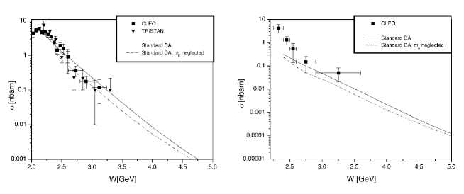
Figure 1: Integrated $\gamma\gamma\rightarrow p\bar{p}$ (left) and $\gamma\gamma\rightarrow\Lambda\bar{\Lambda}$ (right) cross sections ($|\cos(\theta_{\rm cm})|\leq 0.6$) vs. $W=\sqrt{s}$. Solid (dash-dotted) line: predictions obtained with the standard parameterization of the diquark model (cf. Ref. [1]) with (without) mass corrections. Data are taken from Refs. [7, 8, 9].

The model, as applied in Refs. [1, 2, 3, 4], comprises scalar (S) as well as axial-vector (V) diquarks. V-diquarks are important if one wants to describe spin observables which require the flip of baryonic helicities. For the Feynman rules of electromagnetically and strongly interacting diquarks, as well as for the choice of the quark-diquark distribution amplitudes of octet baryons we refer to Ref. [1]. Here it is only important to mention that the composite nature of diquarks is taken into account by multiplying each of the Feynman diagrams entering the hard scattering amplitude with diquark form factors. These are parameterized by multipole functions with the power chosen in such a way that in the limit $p_{\perp}\rightarrow\infty$ the scaling behavior of the pure quark HSF is recovered.

We want to present here a very recent application of the diquark model concerning the class of reactions $\gamma\gamma\rightarrow B\bar{B}$, where $B$ represents an octet baryon. In contrast to foregoing work, we have now considered these processes within the full model including also vector-diquarks. Furthermore, baryon-mass effects are taken into account in a rigorous way by means of a systematic expansion in the parameter (baryon mass/photon energy). With the same set of model parameters as in Refs. [1, 2, 3, 4] we find that the integrated cross-section data (available only) for the $p$-$\bar{p}$ and the $\Lambda$-$\bar{\Lambda}$ channel are very well reproduced (cf. Fig. 1). By comparing the solid and the dash-dotted line it can also be observed that in the few-GeV range baryon-mass effects are still sizable. For details of the calculation and results for other octet-baryon channels we refer to Ref. [6].

Table 1: Decomposition of the proton magnetic form factor into diquark contributions for the proton DA proposed by Chernyak et al. [10]. $S^{I}[q_{1}q_{2}]$ and $V^{I}_{h}[q_{1}q_{2}]$ denote scalar and vector diquarks (with isospin $I$ and helicity $h$), respectively, consisting of quarks $q_{1}$ and $q_{2}$. The various diquark contributions are further decomposed into a 3- and 4-point part, $G_{\rm M}^{3,{\rm p}}$ and $G_{\rm M}^{4,{\rm p}}$, depending on whether one or two gauge bosons couple to the diquark. The constant $C=1.266$ is chosen in such a way that the largest contribution, i.e. the $S^{0}[ud]\rightarrow S^{0}[ud]$ transition, becomes 1.

Transition	$C^{-1}Q^{4}G_{\rm M}^{3,{\rm p}}$	$C^{-1}Q^{4}G_{\rm M}^{4,{\rm p}}$	Sum
$V_{0}^{1}[ud]\rightarrow V_{0}^{1}[ud]$	0.016	0.003	0.019
$V_{0}^{1}[ud]\leftrightarrow V_{0}^{0}[ud]$	0	0.004	0.004
$V_{0}^{1}[ud]\leftrightarrow S^{1}[ud]$	0	0	0
$V_{0}^{1}[ud]\leftrightarrow S^{0}[ud]$	0	-0.063	-0.063
$V_{0}^{0}[ud]\rightarrow V_{0}^{0}[ud]$	0.001	0	0.001
$V_{0}^{0}[ud]\leftrightarrow S^{1}[ud]$	0	-0.002	-0.002
$V_{0}^{0}[ud]\leftrightarrow S^{0}[ud]$	0	-0.011	-0.011
$S^{1}[ud]\rightarrow S^{1}[ud]$	$\approx 0$	$\approx 0$	0.001
$S^{1}[ud]\leftrightarrow S^{0}[ud]$	0	-0.002	-0.002
$S^{0}[ud]\rightarrow S^{0}[ud]$	1.000	-0.005	0.995
$V^{1}_{1}[ud]\rightarrow V^{1}_{1}[ud]$	0	-0.002	-0.002
$V^{1}_{1}[ud]\leftrightarrow V^{0}_{1}[ud]$	0	0.036	0.036
$V^{0}_{1}[ud]\rightarrow V^{0}_{1}[ud]$	0	0.007	0.007
$V_{0}^{1}[uu]\rightarrow V_{0}^{1}[uu]$	-0.016	0.027	0.012
$V^{1}_{0}[uu]\leftrightarrow S^{1}[uu]$	0	-0.003	-0.003
$S^{1}[uu]\rightarrow S^{1}[uu]$	$\approx 0$	0.005	0.004
$V^{1}_{1}[uu]\rightarrow V^{1}_{1}[uu]$	0	-0.013	-0.013
Total			0.985

As the applications mentioned above demonstrate, diquarks are obviously a very useful phenomenological concept (not only) in the field of hard hadronic processes. Physically speaking, diquarks represent effective particles which describe strong quark-quark correlations in baryonic wave functions. Within the pure quark HSF such correlations seem indeed necessary to obtain reasonable results, even for the simplest exclusive observables such as the nucleon magnetic form factors [10]. A more formal justification of diquarks can be obtained by observing that the diquark model should evolve into the pure quark HSF in the limit of asymptotically large momentum transfers. This suggests a reformulation of the pure quark HSF in terms of quark and diquark degrees of freedom. Two obvious constraints for this reformulation are that the leading order hard-scattering amplitude on the quark-diquark level should also consist only of tree graphs (like in the pure quark HSF) and that the result of this reformulation should be independent of the choice of the two quarks which are grouped to a diquark. It has been proved in Ref. [11] that a reformulation of the pure quark HSF fulfilling both constraints is indeed possible. If we employ this reformulation to analyze the proton magnetic form factor with respect to its diquark content, we find the isospin $0$ scalar $S[ud]$ diquark to provide the by far most important contribution (cf. Tab. 1). This is not only the case for the proton DA proposed by Chernyak et al. but holds also for other DA models.

The reformulation of the pure quark HSF in terms of quarks and diquarks requires to study the general Lorentz structure of two-quark subgraphs to obtain the Lorentz covariants and corresponding (Lorentz-invariant) vertex functions of the various gauge-boson diquark vertices. This gives valuable clues how gauge-boson diquark vertices and corresponding form factors could be improved in the naive diquark model. However, in order to arrive at an effective model in the sense that it reproduces the results of the pure quark HSF (and not only the scaling behavior) in the limit of asymptotically large momentum transfers one should take these vertices literally and use the vertex-function results as asymptotic constraints for the parameterization of the diquark form factors. A corresponding program is presently carried out.

References

- [1] R. Jakob, P. Kroll, M. Schürmann, and W. Schweiger, Z. Phys. A 347 (1993) 109;
- [2] P. Kroll, T. Pilsner, M. Schürmann, and W. Schweiger, Phys. Lett. B 316 (1993) 546;
- [3] P. Kroll, M. Schürmann, and P. Guichon, Nucl. Phys. A 598 (1996) 435;
- [4] P. Kroll, M. Schürmann, K. Passek, and W. Schweiger, Phys. Rev. D 55 (1997) 4315;
- [5] See, e.g., S. J. Brodsky and G. P. Lepage, in Perturbative Quantum Chromodynamics, ed. by A. H. Mueller (World Scientific, Singapore, 1989);
- [6] C. F. Berger, diploma thesis, Technological University Graz (1997);
- [7] M. Artuso et al., Phys. Rev. D 50 (1994) 5484;
- [8] H. Hamasaki et al., Phys. Lett B 407 (1997) 185;
- [9] S. Anderson et al., Phys. Rev. D 56 (1997) 2485;
- [10] V. Chernyak, A. Ogloblin, and I. Zhitnitsky, Z. Phys. C 42 (1989) 569;
- [11] B. Lechner, diploma thesis, University Graz (1997).