Abstract

We study the processes $gg\to{\tilde{q}}_{1}{\tilde{q}}_{2}^{*}A$, with $q=t,b$, within the theoretical framework of the Supergravity (SUGRA) inspired Minimal Supersymmetric Standard Model (MSSM) at the leading order (LO) in perturbative Quantum Chromo-Dynamics (QCD). Other than constituting a novel production mechanism of the neutral, CP-odd Higgs particle, they also allow one to relate the size of the corresponding production rates to the ratio of the vacuum expectation values of the two Higgs fields $\tan\beta$, to the trilinear couplings $A_{0}$ and to the sign of the Higgsino mass term $\mathrm{sign}(\mu)$. This interplay is made easier by the absence of any mixing in the ${\tilde{q}}_{1}{\tilde{q}}_{2}A$ vertices, contrary to the case of all other Higgs bosons of the theory.

1 Introduction and motivation

The CP-attribute of the pseudoscalar Higgs boson induces several other oddities in its behaviours, with respect to all other Higgs scalars of the MSSM, that render such a particle a very attractive candidate for phenomenological studies.

For example, in the $qqA$ Feynman rule, where $q$ represents an ordinary heavy quark (hereafter, $q=t,b$), there is no dependence on the Higgs mixing angle, $\alpha$, contrary to the case of the CP-even scalars, $H$ and $h$. As for the charged Higgs, in the $q\bar{q}^{\prime}H^{\pm}$ vertex, another mixing, this time in the quark sector, is introduced via the Cabibbo-Kobayashi-Maskawa matrix. A neat consequence of this is the steep rise(fall) of the production cross sections of the $A$ boson whenever this is emitted by a heavy down(up)-type quark, for increasing(decreasing) $\tan\beta(\cot\beta)$ [1]. For all the other Higgs scalars, such monotonic behaviour is spoiled by the presence of angular terms, typically sines and cosines of $\alpha$, so that only in extreme regions of the MSSM parameter space such peculiar dependence on $\beta$ can be recovered.

If one further considers the Higgs couplings to the scalar partners of ordinary heavy quarks in Supersymmetric (SUSY) theories, the left- and right-handed squarks $\tilde{q}_{\chi}$, with $\chi=R,L$, then it is easy to verify that mixing angles relating their chiral and physical mass eigenvalues do not enter the ${\tilde{q}}_{1}{\tilde{q}}_{2}A$ vertex, i.e., the one involving the observable squarks (the subscript 1(2) referring to the lightest(heaviest) of them). Indeed, this is not the case for the corresponding couplings of the $H$, $h$ and $H^{\pm}$ scalars.

One can see this in the context of SUGRA models [2], with the minimal particle content typical of the MSSM (henceforth denoted as M-SUGRA, the environment we choose for our analysis) [3, 4], where the relevant Feynman rules for the squark-squark-Higgs vertices can be written in the physical basis $\tilde{q}_{1,2}$ as follows :

$$\lambda_{\Phi\tilde{q}_{1}\tilde{q}^{\prime}_{1}} = c_{q}c_{q^{\prime}}\lambda_{\Phi\tilde{q}_{L}\tilde{q}^{\prime}_{L}}+s_{q}s_{q^{\prime}}\lambda_{\Phi\tilde{q}_{R}\tilde{q}^{\prime}_{R}}+c_{q}s_{q^{\prime}}\lambda_{\Phi\tilde{q}_{L}\tilde{q}^{\prime}_{R}}+s_{q}c_{q^{\prime}}\lambda_{\Phi\tilde{q}_{R}\tilde{q}^{\prime}_{L}},$$

$$\lambda_{\Phi\tilde{q}_{2}\tilde{q}^{\prime}_{2}} = s_{q}s_{q^{\prime}}\lambda_{\Phi\tilde{q}_{L}\tilde{q}^{\prime}_{L}}+c_{q}c_{q^{\prime}}\lambda_{\Phi\tilde{q}_{R}\tilde{q}^{\prime}_{R}}-s_{q}c_{q^{\prime}}\lambda_{\Phi\tilde{q}_{L}\tilde{q}^{\prime}_{R}}-c_{q}s_{q^{\prime}}\lambda_{\Phi\tilde{q}_{R}\tilde{q}^{\prime}_{L}},$$

$$\lambda_{\Phi\tilde{q}_{1}\tilde{q}^{\prime}_{2}} = -c_{q}s_{q^{\prime}}\lambda_{\Phi\tilde{q}_{L}\tilde{q}^{\prime}_{L}}+s_{q}c_{q^{\prime}}\lambda_{\Phi\tilde{q}_{R}\tilde{q}^{\prime}_{R}}+c_{q}c_{q^{\prime}}\lambda_{\Phi\tilde{q}_{L}\tilde{q}^{\prime}_{R}}-s_{q}s_{q^{\prime}}\lambda_{\Phi\tilde{q}_{R}\tilde{q}^{\prime}_{L}},$$

$$\lambda_{\Phi\tilde{q}_{2}\tilde{q}^{\prime}_{1}} = -s_{q}c_{q^{\prime}}\lambda_{\Phi\tilde{q}_{L}\tilde{q}^{\prime}_{L}}+c_{q}s_{q^{\prime}}\lambda_{\Phi\tilde{q}_{R}\tilde{q}^{\prime}_{R}}-s_{q}s_{q^{\prime}}\lambda_{\Phi\tilde{q}_{L}\tilde{q}^{\prime}_{R}}+c_{q}c_{q^{\prime}}\lambda_{\Phi\tilde{q}_{R}\tilde{q}^{\prime}_{L}}.$$ (1)

Here, the symbol $\Phi$ denotes cumulatively the five Higgs scalars of the MSSM, $\Phi=H,h,A,$ and $H^{\pm}$. All the $\lambda_{\Phi\tilde{q}_{\chi}\tilde{q}^{\prime}_{\chi^{\prime}}}$’s appearing in eq. (1) can be found, e.g., in the Appendix of Ref. [1]. These are function of the five independent parameters defining the M-SUGRA model: the universal scalar and gaugino masses $M_{0}$ and $M_{1/2}$, the universal trilinear breaking terms $A_{0}$, the ratio of the vacuum expectation values (VEVs) of the two Higgs fields $\tan\beta\equiv v/v^{\prime}$, and the sign of the Higgsino mass term $\mu$.

The squarks mixing angles too, i.e., $\theta_{q}$, with $q=t,b$, can be written in terms of the above four M-SUGRA parameters, as (here, $s_{q}\equiv\sin\theta_{q}$ and $c_{q}\equiv\cos\theta_{q}$)

$$\tan(2\theta_{b}) = \frac{2m_{b}(A_{b}+\mu\tan\beta)}{M_{\tilde{Q}_{3}}^{2}-M_{\tilde{D}_{3}}^{2}+(-\frac{1}{2}+\frac{2s_{W}^{2}}{3})M_{Z}^{2}\cos 2\beta},$$

$$\tan(2\theta_{t}) = \frac{2m_{t}(A_{t}+\mu\cot\beta)}{M_{\tilde{Q}_{3}}^{2}-M_{\tilde{U}_{3}}^{2}+(\frac{1}{2}-\frac{4s_{W}^{2}}{3})M_{Z}^{2}\cos 2\beta},$$ (2)

with $M_{Z}$ the $Z$-boson mass and $s^{2}_{W}\equiv\sin^{2}\theta_{W}$ the (squared) Weinberg angle, $m_{t}$ and $m_{b}$ the top and bottom masses, where $A_{t}$ and $A_{b}$ are the mentioned (top and bottom) trilinear couplings at the EW scale, while $M_{\tilde{Q}_{3}}$, $M_{\tilde{U}_{3}}$ and $M_{\tilde{D}_{3}}$ are the running soft SUSY breaking squark masses of the third generation, as obtained from starting their evolution at a common Grand Unification Theory (GUT) scale set equal to $M_{0}$.

Now, it should be noticed that in the case of the CP-odd Higgs boson, i.e., $\Phi=A$, if one reverts the chirality flow in the vertex $\lambda_{A\tilde{q}_{L}\tilde{q}_{R}}$, the corresponding Feynman rule changes its sign [1],

$$\lambda_{A\tilde{q}_{L}\tilde{q}_{R}}=-\lambda_{A\tilde{q}_{R}\tilde{q}_{L}},$$ (3)

so that, by making use of eq. (1) (where $\lambda_{A\tilde{q}_{1}\tilde{q}_{1}}=\lambda_{A\tilde{q}_{2}\tilde{q}_{2}}=0$ [1]), one can conclude that the vertices $\lambda_{A\tilde{t}_{1}\tilde{t}_{2}}$ and $\lambda_{A\tilde{b}_{1}\tilde{b}_{2}}$ are independent of the mixing angles $\theta_{t}$ and $\theta_{b}$. In fact, the Feynman rules for those vertices reduce to (here, $g_{W}^{2}=4\pi\alpha_{\mathrm{em}}/s^{2}_{W}$ and $M_{W}^{2}=M_{Z}^{2}(1-s^{2}_{W})$)

$$\lambda_{A\tilde{t}_{1}\tilde{t}_{2}}=-\frac{g_{W}m_{t}}{2M_{W}}\left(\mu-A_{t}\cot\beta\right),\qquad\qquad\lambda_{A\tilde{b}_{1}\tilde{b}_{2}}=-\frac{g_{W}m_{b}}{2M_{W}}\left(\mu-A_{b}\tan\beta\right).$$ (4)

These are precisely the couplings entering the processes that we are going to discuss:

$$gg\to{\tilde{q}}_{1}{\tilde{q}}_{2}^{*}A,\qquad\qquad q=t,b.$$ (5)

It should by now be obvious to the reader our intent in this paper. Namely, to study the dependence of the production rates of the scattering processes (5) on the low-energy SUSY parameters, in order to pin down their actual value at the GUT scale, thus constraining the SUSY scenario which lies behind the MSSM, through experimental measurements of physical observables.

Needless to say, such a task is greatly facilitated in case of pseudoscalar Higgs production, $\Phi=A$, as we have just shown that the vertex expressions for the other cases, when $\Phi=H,h$ and $H^{\pm}$, are much more involved (i.e., they contain as additional free parameters the Higgs and squark mixing angles), so that it is inevitably much more difficult to extract useful information from the corresponding production rates. However, given that the final signatures of all possible ‘gluon gluon $\to$ squark-squark-Higgs’ processes, after the decays of the heavy objects, are at times very similar, one cannot subtract oneself from studying the whole of such a phenomenology. This is beyond the scope of this short note, though, and we will address the problem in a forthcoming publication [6]. Furthermore, in that paper, we will also discuss more closely another relevant aspect of Higgs production in association with heavy squark pairs, that is, the fact that such processes can furnish additional production mechanisms of Higgs bosons, to be exploited in the quest for such elusive particles, somewhat along the lines of Ref. [7], where the final state with both light Higgs, $h$, and stop pairs, ${\tilde{t}}_{1}{\tilde{t}}_{1}^{*}$, was considered. Finally, notice that, given the current limits on squark and Higgs masses [8, 9], the only collider environment able to produce a statistically significative number of events (5) is the LHC ($\sqrt{s}=14$ TeV), to which we confine our analysis. Incidentally, at such a machine, the contribution to squark-squark-Higgs production via quark-antiquark annihilations is negligible compared to the gluon-gluon induced rates [7], so we will not consider the former here.

The plan of this letter is as follows. The next Section briefly outlines how we have performed the calculations. In Sect. 3 we present and discuss our findings. The conclusions are in the last Section.

2 Calculation

The techniques adopted to calculate our processes will be described in detail in Ref. [6], where also the formulae necessary for the numerical computation of the Feynman amplitudes will be given. Here, we only sketch the procedure, for completeness.

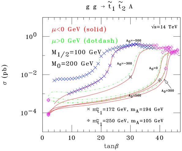
Figure 1: Total cross sections for process $gg\rightarrow\tilde{t}_{1}\tilde{t}_{2}^{*}A$ as a function of $\tan\beta$. These are plotted for both positive (dotdash) and negative (solid) values of $\mu$ and for a selection of $A_{0}$ values. (The other M-SUGRA parameters have been chosen as $M_{0}=200$ GeV and $M_{1/2}=100$ GeV.) The symbol “ $\diamond$ ($\times$) ” is used to indicate data points forbidden by experimental bounds from direct searches of the lightest Higgs(squark) scalar, yielding $2\lower 3.01385pt\hbox{$\;\stackrel{{\scriptstyle\textstyle<}}{{\sim}}\;$}\tan\beta\lower 3.01385pt\hbox{$\;\stackrel{{\scriptstyle\textstyle<}}{{\sim}}\;$}40$($m_{{\tilde{t}}_{1}}>120$ GeV). Two points with the masses of the lightest stop and the CP-odd Higgs are also shown.

There are 10 LO Feynman diagrams for each of the two processes (5): see Fig. 1 of [7] for the relevant topologies. These have been calculated analytically and integrated numerically over a three-body phase space. While doing so, they have been convoluted with gluon Parton Distribution Functions (PDFs), as provided by the LO set CTEQ(4L) [10].

The centre-of-mass (CM) energy at the partonic level was the scale used to evaluate both the PDFs and the strong coupling constant, $\alpha_{\mathrm{s}}$. We have used the two-loop scaling for the latter, with all relevant thresholds [12] onset within the MSSM (as these are spanned through the $Q^{2}$ evolution of the structure functions), in order to match the procedure we have adopted in generating the other couplings, these also produced via the two-loop RGEs [13].

Depending on the relative value of the final state masses in (5), whether $m_{{\tilde{q}}_{2}}$ is larger or smaller than $(m_{{\tilde{q}}_{1}}+m_{A})$, the production of the pseudoscalar Higgs boson can be regarded as taking place either via a decay or a bremsstrahlung channel. We have treated the two processes on the same footing, without making any attempt to separate them, as for the time being we are only interested in the total production rates of the 2 $\to$ 3 processes (5). In this respect, it should be mentioned that the partial widths entering in our MEs are significantly smaller than the total decay widths, so that processes (5) do retain the dynamics of the squark-squark-Higgs production vertices also at decay level.

Regarding the numerical values of the M-SUGRA parameters adopted in this paper, we have proceeded as follows. For a start, we have set $M_{0}=200$ GeV and $M_{1/2}=100$ GeV. For such a choice, the M-SUGRA model predicts squark and Higgs masses in the region of 100–400 GeV, so that the latter can in principle materialise at LHC energies. Then, we have varied the trilinear soft SUSY breaking parameter $A_{0}$ in a large region, $(-500,500)$ GeV, while we have spanned the $\tan\beta$ value between 2 and 45. As for $\mu$, whereas in our model its magnitude is constrained, its sign is not. Thus, in all generality, we have explored both the possibilities $\mathrm{sign}(\mu)=\pm$. Finally, we have gone back to consider $M_{0}$ and $M_{1/2}$ in other mass regions.

Starting from the five M-SUGRA parameters $M_{0}$, $M_{1/2}$, $A_{0}$, $\tan\beta$ and ${\mbox{sign}}(\mu)$, we have generated the spectrum of masses, widths, couplings and mixings relative to squarks and Higgs particles entering reactions (5) by running the ISASUGRA/ISASUSY programs for M-SUGRA contained in the latest release of the package ISAJET [13]. The default value of the top mass we have used was 175 GeV. Finally, note that also typical EW parameters, such as $\alpha_{\mathrm{em}}$ and $\sin^{2}\theta_{W}$, are taken from this program.

3 Results

Although we will in this letter mainly concentrate on the case of CP-odd Higgs production, we nonetheless ought to display some typical cross sections for all processes of the form [6]

$$g~{}g~{}\rightarrow~{}{\tilde{q}}_{\chi}~{}{\tilde{q}}^{{}^{\prime}*}_{\chi^{\prime}}~{}\Phi,$$ (6)

where $q^{(^{\prime})}=t,b$, $\chi^{(^{\prime})}=1,2$ and $\Phi=H,h,A,H^{\pm}$. This is done in Tab. I, where, for reference, the trilinear coupling $A_{0}$ has been set to zero and two extremes values of $\tan\beta$, i.e., $2$ and $40$, have been selected. The corresponding mass spectrum for the particles in the final state of processes (6) is given in Tab. II. There, it is well worth noticing that modifying the value of $\tan\beta$ corresponds to induce quite different mass values for both Higgs bosons and squarks.

From Tab. I, one can notice that our two processes could well yield detectable rates in the large $\tan\beta$ region. For a LHC running at high luminosity, some seven thousand such events can be produced per year. For large $\tan\beta$ values, alongside pseudoscalar Higgs boson production, there are at least three other mechanisms (6) with observable rates, as one finds that, typically:

$$\sigma(gg\rightarrow\tilde{t}_{1}\tilde{t}_{2}^{*}H;~{}gg\rightarrow\tilde{t}_{1}\tilde{t}_{1}^{*}h;~{}gg\rightarrow\tilde{t}_{1}\tilde{t}_{2}^{*}h;~{}gg\rightarrow\tilde{t}_{1}\tilde{t}_{2}^{*}A;~{}gg\rightarrow\tilde{b}_{1}\tilde{b}_{2}^{*}A)\lower 3.01385pt\hbox{$\;\stackrel{{\scriptstyle\textstyle>}}{{\sim}}\;$}10^{-2}\;{\rm pb}.$$ (7)

Among these, it is $gg\rightarrow\tilde{t}_{1}\tilde{t}_{2}^{*}H$ that shows a strong dependence on $\mathrm{sign}(\mu)$, whereas all other reactions in (7) are rather stable against variations of the latter.

$$\begin{array}[]{|c|c|c|c|c|}\hline\cr\sigma\;{\mathrm{(pb)}}&\tan\beta=2,\mu>0&\tan\beta=2,\mu<0&\tan\beta=40,\mu>0&\tan\beta=40,\mu<0\\[5.69054pt] \hline\cr\sigma(gg\rightarrow\tilde{t}_{1}\tilde{t}_{1}^{*}H)&3.3\times 10^{-4}&3.6\times 10^{-5}&4.7\times 10^{-5}&5.1\times 10^{-5}\\[5.69054pt] \hline\cr\sigma(gg\rightarrow\tilde{t}_{2}\tilde{t}_{2}^{*}H)&2.1\times 10^{-5}&1.9\times 10^{-5}&5.2\times 10^{-6}&6.2\times 10^{-6}\\[5.69054pt] \hline\cr\sigma(gg\rightarrow\tilde{t}_{1}\tilde{t}_{2}^{*}H)&4.6\times 10^{-4}&2.6\times 10^{-5}&1.2\times 10^{-2}&4.6\times 10^{-3}\\[5.69054pt] \hline\cr\sigma(gg\rightarrow\tilde{b}_{1}\tilde{b}_{1}^{*}H)&3.0\times 10^{-6}&2.8\times 10^{-6}&2.0\times 10^{-6}&1.7\times 10^{-6}\\[5.69054pt] \hline\cr\sigma(gg\rightarrow\tilde{b}_{2}\tilde{b}_{2}^{*}H)&5.1\times 10^{-8}&4.9\times 10^{-8}&1.0\times 10^{-6}&1.1\times 10^{-6}\\[5.69054pt] \hline\cr\sigma(gg\rightarrow\tilde{b}_{1}\tilde{b}_{2}^{*}H)&1.3\times 10^{-6}&1.9\times 10^{-7}&4.1\times 10^{-3}&3.1\times 10^{-3}\\[5.69054pt] \hline\cr\sigma(gg\rightarrow\tilde{t}_{1}\tilde{t}_{1}^{*}h)&2.2\times 10^{-1}&1.8\times 10^{-2}&1.4\times 10^{-2}&1.4\times 10^{-2}\\[5.69054pt] \hline\cr\sigma(gg\rightarrow\tilde{t}_{2}\tilde{t}_{2}^{*}h)&3.6\times 10^{-3}&5.5\times 10^{-3}&1.4\times 10^{-3}&1.5\times 10^{-3}\\[5.69054pt] \hline\cr\sigma(gg\rightarrow\tilde{t}_{1}\tilde{t}_{2}^{*}h)&1.7\times 10^{-2}&2.8\times 10^{-2}&7.4\times 10^{-2}&9.3\times 10^{-2}\\[5.69054pt] \hline\cr\sigma(gg\rightarrow\tilde{b}_{1}\tilde{b}_{1}^{*}h)&1.2\times 10^{-4}&1.5\times 10^{-4}&2.0\times 10^{-4}&1.8\times 10^{-4}\\[5.69054pt] \hline\cr\sigma(gg\rightarrow\tilde{b}_{2}\tilde{b}_{2}^{*}h)&2.0\times 10^{-6}&2.6\times 10^{-6}&1.4\times 10^{-6}&1.5\times 10^{-6}\\[5.69054pt] \hline\cr\sigma(gg\rightarrow\tilde{b}_{1}\tilde{b}_{2}^{*}h)&3.4\times 10^{-6}&1.2\times 10^{-4}&2.4\times 10^{-3}&3.3\times 10^{-3}\\[5.69054pt] \hline\cr\sigma(gg\rightarrow\tilde{t}_{1}\tilde{t}_{2}^{*}A)&5.7\times 10^{-4}&7.7\times 10^{-5}&2.9\times 10^{-2}&1.7\times 10^{-2}\\[5.69054pt] \hline\cr\sigma(gg\rightarrow\tilde{b}_{1}\tilde{b}_{2}^{*}A)&1.3\times 10^{-6}&2.4\times 10^{-7}&1.3\times 10^{-2}&1.2\times 10^{-2}\\[5.69054pt] \hline\cr\sigma(gg\rightarrow\tilde{t}_{1}\tilde{b}_{1}^{*}H^{-})&4.3\times 10^{-5}&1.4\times 10^{-5}&5.0\times 10^{-6}&4.8\times 10^{-6}\\[5.69054pt] \hline\cr\sigma(gg\rightarrow\tilde{t}_{2}\tilde{b}_{2}^{*}H^{-})&2.7\times 10^{-7}&2.5\times 10^{-7}&5.0\times 10^{-4}&5.4\times 10^{-4}\\[5.69054pt] \hline\cr\sigma(gg\rightarrow\tilde{t}_{1}\tilde{b}_{2}^{*}H^{-})&5.6\times 10^{-6}&3.2\times 10^{-7}&4.5\times 10^{-3}&4.2\times 10^{-3}\\[5.69054pt] \hline\cr\sigma(gg\rightarrow\tilde{t}_{2}\tilde{b}_{1}^{*}H^{-})&3.7\times 10^{-4}&7.9\times 10^{-5}&2.1\times 10^{-3}&1.7\times 10^{-3}\\[5.69054pt] \hline\cr\end{array}$$ (27)

Table I: Total cross sections for processes of the type $g~{}g~{}\rightarrow~{}{\tilde{q}}_{\chi}~{}{\tilde{q}}^{{}^{\prime}*}_{\chi^{\prime}}~{}\Phi$, where $q^{(^{\prime})}=b,t$, $\chi^{(^{\prime})}=1,2$ and $\Phi=H,h,A,H^{\pm}$, in the MSSM, at the leading order in perturbative QCD, for selected values of $\tan\beta$ and $\mathrm{sign}(\mu)$. The other three independent parameters of the model have been set as: $M_{0}=200$ GeV, $M_{1/2}=100$ GeV and $A_{0}=0$.

At low $\tan\beta$’s, the cross sections for pseudoscalar Higgs boson production are presumably too poor to be of great experimental help, in both cases of sbottom and stop squark production. Even assuming 100 fb^-1 of accumulated luminosity per year at the LHC, only a handful of events of the form (5) can be produced, if $A_{0}\approx 0$, mainly through the $gg\rightarrow\tilde{t}_{1}\tilde{t}_{2}^{*}A$ channel. (Prospects are somewhat more optimistic if the common trilinear coupling is much smaller than zero, but in the case of stop squarks only: we will come back to this point later on.) Anyhow, for small $\tan\beta$ values, the three channels $gg\rightarrow\tilde{t}_{\chi}\tilde{t}_{\chi^{\prime}}^{*}h$ can boast very large production rates. Moreover, the dominant one, when $\chi=\chi^{\prime}=1$, exhibits a strong sensitivity on the sign of $\mu$, as the two cross sections obtained for $\mathrm{sign}(\mu)=\pm$ differ by about an order of magnitude.

Therefore, both in the low and high $\tan\beta$ regime, pseudoscalar Higgs boson production is in general less effective than other channels in constraining the sign of the Higgsino mass term. This aspect will however not be investigated any further here, as it will be addressed in detail in forthcoming Ref. [6]. In fact, here we are more concerned with the fact that reactions (5) are very sensitive to $\tan\beta$, much more than any other squark-squark-Higgs production channel: compare the first two columns in Tab. I with the last two, particularly for $gg\to\tilde{b}_{1}\tilde{b}_{2}^{*}A$ (differences are over four/five orders of magnitude !). Other competitive mechanisms in this respect are (in the observable region, say, with a cross section above $10^{-3}$ pb): $gg\to\tilde{t}_{1}\tilde{t}_{2}^{*}H$, $gg\to\tilde{b}_{1}\tilde{b}_{2}^{*}H$ and $gg\to\tilde{t}_{1}\tilde{b}_{2}^{*}H^{-}$. They are however suppressed, in general, as compared to the two CP-odd production channels, so for the time being we leave them aside for future studies [6] and concentrate exclusively on processes (5).

$$\begin{array}[]{|c|c|c|c|c|}\hline\cr{\rm Masses}\;({\mathrm{GeV}})&\tan\beta=2,\mu>0&\tan\beta=2,\mu<0&\tan\beta=40,\mu>0&\tan\beta=40,\mu<0\\[5.69054pt] \hline\cr m_{\tilde{t}_{1}}&171&258&221&224\\[5.69054pt] \hline\cr m_{\tilde{t}_{2}}&374&320&349&348\\[5.69054pt] \hline\cr m_{\tilde{b}_{1}}&275&275&222&226\\[5.69054pt] \hline\cr m_{\tilde{b}_{2}}&314&314&306&303\\[5.69054pt] \hline\cr m_{H}&382&385&128&126\\[5.69054pt] \hline\cr m_{h}&81&69^{*}&104&103\\[5.69054pt] \hline\cr m_{A}&375&377&128&126\\[5.69054pt] \hline\cr m_{H^{\pm}}&383&385&155&153\\[5.69054pt] \hline\cr\end{array}$$ (37)

Table II: Masses of stop and sbottom squarks and Higgs bosons in the MSSM in the small and large $\tan\beta$ region, for both positive and negative values of $\mu$ and universal boundary conditions: $M_{0}=200$ GeV, $M_{1/2}$=100 GeV and $A_{0}=0$.
^∗ This value is actually excluded from the latest LEP bounds on the light and CP-odd Higgs boson masses [9]: $m_{h},m_{A}\lower 2.41109pt\hbox{$\;\stackrel{{\scriptstyle\textstyle>}}{{\sim}}\;$}80$ GeV. Nonetheless we keep it here for illustrative purposes, as representative of the condition $m_{A}\gg m_{h}$, typical of the small $\tan\beta$ regime.

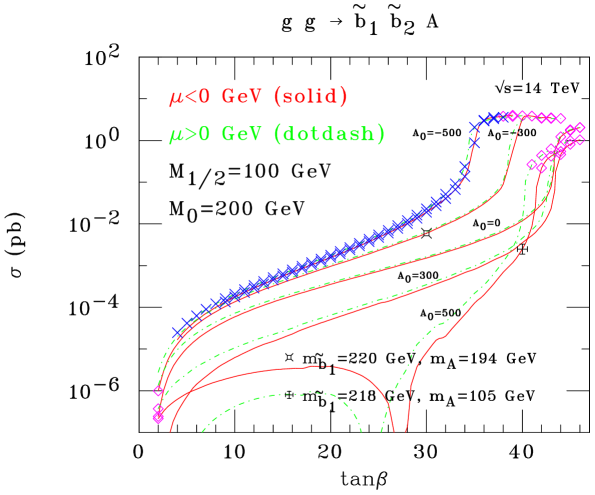
Figure 2: Same as in Fig. 1 for process $gg\rightarrow\tilde{b}_{1}\tilde{b}_{2}^{*}A$.

Figs. 1 and 2 further enlighten the $\tan\beta$ dependence of pseudoscalar Higgs boson production, in association with stop and sbottom squarks, respectively, as we have now treated $A_{0}$ as a variable parameter. Indeed, the typical behaviour seen in Tab. I for $A_{0}=0$ in $gg\to\tilde{t}_{1}\tilde{t}_{2}^{*}A$ and $gg\to\tilde{b}_{1}\tilde{b}_{2}^{*}A$ persists for all other values of $A_{0}$ considered.

The variation with $\tan\beta$, and particularly the steep rise at high values of the latter, can be understood in the following terms. For large $\tan\beta$, the squark-squark Higgs boson couplings of eq. (4) can be rewritten in the form

$$\lambda_{A\tilde{t}_{1}\tilde{t}_{2}}\simeq-\frac{g_{W}m_{t}}{2M_{W}}\mu,\qquad\qquad\lambda_{A\tilde{b}_{1}\tilde{b}_{2}}\simeq-\frac{g_{W}m_{b}}{2M_{W}}A_{b}\tan\beta.$$ (38)

That is, the coupling which is associated with the sbottom pair is proportional to $\tan\beta$, so that, eventually, the total $\tilde{b}_{1}\tilde{b}_{2}^{*}A$ cross section will grow with $\tan^{2}\beta$ while the coupling related to the stop pair takes on constant values. In the latter, the enhancement of the $\tilde{t}_{1}\tilde{t}_{2}^{*}A$ cross section with $\tan\beta$ is rather a phase space effect since, as $\tan\beta$ increases, the CP-odd Higgs boson mass decreases considerably (the squark masses changing much less instead), as we can see from Tab. II. Of course the same is valid in the former case and that is why our Figs. 1–2 follow the pattern $\sigma(gg\rightarrow\tilde{b}_{1}\tilde{b}_{2}^{*}A)\lower 3.01385pt\hbox{$\;\stackrel{{\scriptstyle\textstyle>}}{{\sim}}\;$}\sigma(gg\rightarrow\tilde{t}_{1}\tilde{t}_{2}^{*}A)$ at large $\tan\beta$.

Despite of the abundance of $\tilde{t}_{1}\tilde{t}_{2}^{*}A$ and $\tilde{b}_{1}\tilde{b}_{2}^{*}A$ events at large $\tan\beta$, overwhelming contributions involving the light stop ${\tilde{t}}_{1}$ and light Higgs scalar $h$, i.e., $\tilde{t}_{1}\tilde{t}_{1}^{*}h$ and, particularly, $\tilde{t}_{1}\tilde{t}_{2}^{*}h$ (see Tab. I), would however dominate the squark-squark-Higgs production phenomenology. Therefore, it might seem at first glance that reactions (5) cannot possibly be disentangled, further considering that at large $\tan\beta$ the dominant decay modes of both $h$ and $A$ scalars are into $b\bar{b}$ pairs [14]. This need not to be true though. In fact, the reader should recall two important aspects. Firstly, the lighter scalar quark mass, $m_{\tilde{t}_{1}}$, will most likely be known well before a statistically significative sample of events of the form (6) can be collected. It follows that its knowledge can be exploited to remove $gg\to{\tilde{q}}_{\chi}{\tilde{q}}^{{}^{\prime}*}_{\chi^{\prime}}\Phi$ candidates with exactly two light stop squarks, thus also unwanted $\tilde{t}_{1}\tilde{t}_{1}^{*}h$ final states. Secondly, in the $b\bar{b}$ channel, one should expect experimental mass resolutions to be smaller than the typical mass differences $m_{A}-m_{h}\lower 3.01385pt\hbox{$\;\stackrel{{\scriptstyle\textstyle>}}{{\sim}}\;$}20$ GeV seen for $\tan\beta\lower 3.01385pt\hbox{$\;\stackrel{{\scriptstyle\textstyle<}}{{\sim}}\;$}35$ (see Tab. II) [6]. Needless to say, the light scalar $h$ ought to have been discovered (and $m_{h}$ measured) by then, for the sake of the all SUSY theory, so that a suitable selection of $b\bar{b}$ pairs far away from the $m_{h}$ resonance (or, at worse, an event counting operation in the case of overlapping $h$ and $A$ mass peaks, at extremely large $\tan\beta$) would aid to reduce $\tilde{t}_{1}\tilde{t}_{2}^{*}h$ events also.

As for the low $\tan\beta$ region, as intimated a few paragraphs above, we can appreciate in Fig. 1 the beneficial effect of a large and negative value of $A_{0}$, in terms of the $\mathrm{sign}(\mu)$ dependence of the $A$ production rates. For example, for $\tan\beta\sim 2$, the cross sections for $\mu>0$ and $\mu<0$ take very different values, by an order of magnitude. In fact, one has that, for $A_{0}\lower 3.01385pt\hbox{$\;\stackrel{{\scriptstyle\textstyle<}}{{\sim}}\;$}-300$ GeV,

$$\sigma(gg\rightarrow\tilde{t}_{1}\tilde{t}_{2}^{*}A)\sim 10^{-3}~{}{\mathrm{pb}}\;\;\;{\rm for}\;\;\;\mu>0,\qquad\sigma(gg\rightarrow\tilde{t}_{1}\tilde{t}_{2}^{*}A)\sim 10^{-4}~{}{\mathrm{pb}}\;\;\;{\rm for}\;\;\;\mu<0\;.$$ (39)

Therefore, in this scenario one might aim to constrain the actual value of sign($\mu$) from the $\tilde{t}_{1}\tilde{t}_{2}^{*}A$ final states alone, given such a large difference. Unfortunately, the total number of events (after having considered the decay rates, the finite efficiency and resolution of experimental analyses, etc.) is again not so large, so that one would presumably be better off by relying on reaction $gg\rightarrow\tilde{t}_{1}\tilde{t}_{2}^{*}h$. In this respect though, one thing is worth spotting, i.e., the much larger value of $m_{A}$ as compared to $m_{h}$ if $\tan\beta$ is small, see Tab. II. A consequence of this is that the decay patterns of the two Higgs bosons are very different. Whereas the light one would only decay into $b\bar{b}$ pairs, the pseudoscalar one would mainly yield $t\bar{t}$ pairs [14]. Given the huge QCD noise of the LHC, the latter might in the end become a competitive approach, especially if a clean electron/muon tag can be achieved in the (anti)top decays.

But, let us now turn our attention to the other strong dependence of the production rates of $gg\to\tilde{t}_{1}\tilde{t}_{2}^{*}A$ and $gg\to\tilde{b}_{1}\tilde{b}_{2}^{*}A$: the one on the common trilinear coupling $A_{0}$. This is in fact the most noticeable feature of both Figs. 1–2: that the sensitivity to $A_{0}$ of the production cross sections provides the unique possibility of constraining, possibly the sign, and hopefully the magnitude, of this fundamental M-SUGRA parameter. Indeed, we have come to believe that this is the main novelty that should be attributed to the phenomenological potential of the processes we are studying, as one might quite rightly expect that the determination of $\tan\beta$ will come first from studies in the pure Higgs sector (i.e., via SM-like Higgs production and decay mechanisms), especially considering the theoretical upper limit on $m_{h}$. Should this be the case, far from overshadowing the usefulness of reactions (5), the knowledge of $\tan\beta$ would further help to constrain $A_{0}$. Let us see how.

For a start, to observe by the thousand events involving $A$-production with pairs of stop quarks would induce the following reasoning:

$$\sigma(gg\rightarrow\tilde{t}_{1}\tilde{t}_{2}^{*}A)\lower 3.01385pt\hbox{$\;\stackrel{{\scriptstyle\textstyle>}}{{\sim}}\;$}10^{-2}\;{\mathrm{pb}}\Rightarrow\left\{\begin{array}[]{c}-500<A_{0}<0\;\;{\rm for}\;\;22\lower 3.01385pt\hbox{$\;\stackrel{{\scriptstyle\textstyle<}}{{\sim}}\;$}\tan\beta\lower 3.01385pt\hbox{$\;\stackrel{{\scriptstyle\textstyle<}}{{\sim}}\;$}40\;\;{\rm and}\;\;\mu=\pm.\\[8.53581pt] \;\;\,0\leq A_{0}<500\;\;{\rm for}\;\;40\lower 3.01385pt\hbox{$\;\stackrel{{\scriptstyle\textstyle<}}{{\sim}}\;$}\tan\beta\lower 3.01385pt\hbox{$\;\stackrel{{\scriptstyle\textstyle<}}{{\sim}}\;$}42\;\;{\rm and}\;\;\mu=\pm.\end{array}\right.\;$$ (42)

That is to say, unless $40\lower 3.01385pt\hbox{$\;\stackrel{{\scriptstyle\textstyle<}}{{\sim}}\;$}\tan\beta\lower 3.01385pt\hbox{$\;\stackrel{{\scriptstyle\textstyle<}}{{\sim}}\;$}42$ (a very small corner of the M-SUGRA parameter space), to observe such a rate of $\tilde{t}_{1}\tilde{t}_{2}^{*}A$ events would mean that $A_{0}$ is necessarily negative (whichever the sign of $\mu$).

Incidentally, we would like the reader to spot in Fig. 1 that are the lines corresponding to $A_{0}=300$ GeV (denoted by the arrow) those stretching to the far right of the plot, thus inverting the trend of decreasing rates with growing $A_{0}$. In other terms, such curves represent a true lower limit on the value of this cross section (practically for all $\tan\beta$ values), so that the latter is bound to be in the range

$$10^{-4}~{}{\mathrm{pb}}\lower 3.01385pt\hbox{$\;\stackrel{{\scriptstyle\textstyle<}}{{\sim}}\;$}\sigma(gg\rightarrow\tilde{t}_{1}\tilde{t}_{2}^{*}A)\lower 3.01385pt\hbox{$\;\stackrel{{\scriptstyle\textstyle<}}{{\sim}}\;$}10^{-1}\;{\mathrm{pb}}\;,$$ (43)

values well within the reach of the LHC luminosity !

Similarly, one can proceed to analyse $gg\rightarrow\tilde{b}_{1}\tilde{b}_{2}^{*}A$ from Fig. 2. Schematically,

$$\sigma(gg\rightarrow\tilde{b}_{1}\tilde{b}_{2}^{*}A)\lower 3.01385pt\hbox{$\;\stackrel{{\scriptstyle\textstyle>}}{{\sim}}\;$}10^{-2}\;{\mathrm{pb}}\Rightarrow\left\{\begin{array}[]{c}-500<A_{0}<0\;\;{\rm for}\;\;28\lower 3.01385pt\hbox{$\;\stackrel{{\scriptstyle\textstyle<}}{{\sim}}\;$}\tan\beta\lower 3.01385pt\hbox{$\;\stackrel{{\scriptstyle\textstyle<}}{{\sim}}\;$}40\;\;{\rm and}\;\;\mu=\pm.\\[8.53581pt] \;\;\,0\leq A_{0}<500\;\;{\rm for}\;\;40\lower 3.01385pt\hbox{$\;\stackrel{{\scriptstyle\textstyle<}}{{\sim}}\;$}\tan\beta\lower 3.01385pt\hbox{$\;\stackrel{{\scriptstyle\textstyle<}}{{\sim}}\;$}42\;\;{\rm and}\;\;\mu=\pm.\end{array}\right.\;$$ (46)

Once again, to observe $\tilde{b}_{1}\tilde{b}_{2}^{*}A$ signals at such a rate would force $A_{0}$ to be negative over most of the M-SUGRA parameter space.

As for peculiar trends in Fig. 2, two behaviours worth commenting on are the following. Firstly, that the production rates decrease with diminishing $\tan\beta$ much more than they do in case of stop production, particularly if $\tan\beta\lower 3.01385pt\hbox{$\;\stackrel{{\scriptstyle\textstyle<}}{{\sim}}\;$}30$. Secondly, that the cross sections exactly vanish in the case $A_{0}=500$ GeV, when $\tan\beta=24(27)$ if $\mu>0(\mu<0)$, as induced by the $\propto(\mu-A_{b}\tan\beta)$ dependence of the production vertex, when $|\mu|\ll|A_{b}\tan\beta|$ and $A_{b}$ changes its sign.

Another aspect made clear by both these two figures is that current experimental bounds tend to exclude only extreme parameter regions, i.e., where $A_{0}$ is strongly negative and/or where $\tan\beta$ is extremely high. On the one hand, LEP2 has almost exhausted its SUSY discovery potential, as most of the data have already been collected and/or analysed, whereas at Tevatron, the present $m_{\tilde{t}_{1}}\buildrel\scriptscriptstyle>\over{\scriptscriptstyle\sim}120$ GeV limit on the lighter stop mass is unlikely to be increased by the new runs to the typical values of Tab. II. On the other hand, the bulk of the $(A_{0},\tan\beta,\mathrm{sign}(\mu))$ parameter space investigated here, where processes (5) could well be detected and studied at the LHC, appears in Figs. 1–2 far beyond the reach of the present colliders. Therefore, in the very short term, one should not expect that new experimental limits can modify drastically the look of our plots. In particular, notice that the presence of ${\tilde{t}}_{2}$ and ${\tilde{b}}_{2}$ squarks in the final state of processes (5) implies that the corresponding production rates at Tevatron are negligible, even for optimistic luminosities, because of the enormous phase space suppression (see Tab. II). Therefore, we believe that, when the LHC will start running, most of the M-SUGRA parameter space discussed here will still be unexplored.

Bringing together the various results obtained so far on $A_{0}$, $\tan\beta$ and $\mathrm{sign}(\mu)$, we attempt to summarise our findings in Tab. III. There, we list the restrictions that can in principle be deduced on the above three parameters by studying the two processes (5), assuming that none of these quantities is known beforehand. Indeed, an enormous area of the M-SUGRA space can be put under scrutiny, particularly involving $A_{0}$ and $\tan\beta$. The prospect of the latter quantity being already known by the time $gg\to\tilde{t}_{1}\tilde{t}_{2}^{*}A$ and $gg\to\tilde{b}_{1}\tilde{b}_{2}^{*}A$ studies begin would be even more exciting. In such a case, a vertical line could be drawn in Figs. 1–2, so that an accurate measurement of the production cross sections of processes (5) would precisely pin-point the actual value of $A_{0}$.

Before closing, we study the dependence of pseudoscalar Higgs boson production in association with stop and sbottom squarks on the last two M-SUGRA independent parameters: $M_{0}$ and $M_{1/2}$. The main effect of changing the latter is onto the masses of the final state scalars, through the phase space volume as well as via propagator effects in the scattering amplitudes. In other terms, to increase one or the other depletes the typical cross sections of (6), simply because the values of all $m_{\tilde{q}_{\chi}}$ and $m_{\Phi}$ get larger. Tab. IV samples such a trend on four among the dominant production channels, including our two reactions (5). As an example, notice that, for $M_{0}=300$ GeV and $M_{1/2}=250$ GeV, all the squark masses are of the order $\lower 3.01385pt\hbox{$\;\stackrel{{\scriptstyle\textstyle>}}{{\sim}}\;$}460$ GeV, whereas for the heavy Higgs bosons one has that typical values are $\lower 3.01385pt\hbox{$\;\stackrel{{\scriptstyle\textstyle>}}{{\sim}}\;$}290$ GeV. Not surprisingly then, among the processes in Tab. IV, for such high $M_{0}$ and $M_{1/2}$ values, the only ones to survive are those involving both the lightest squark (i.e., $\tilde{t}_{1}$) and the $h$ scalar (for which one necessarily has that $m_{h}\lower 3.01385pt\hbox{$\;\stackrel{{\scriptstyle\textstyle<}}{{\sim}}\;$}130$ GeV) [6, 7]. In comparison, processes (5) are generally suppressed, as one heavy mass $m_{{\tilde{q}}_{2}}$ is always present in the final states and since $m_{A}\lower 3.01385pt\hbox{$\;\stackrel{{\scriptstyle\textstyle>}}{{\sim}}\;$}m_{h}$. Therefore, this last exercise shows that only light $M_{0}$ and $M_{1/2}$ masses (say, below 200 and 150 GeV, respectively) would possibly allow for pseudoscalar production to be detectable at the LHC.

$$\begin{array}[]{|c|c|c|c|c|}\hline\cr\sigma(gg\rightarrow\tilde{t}_{1}\tilde{t}_{2}^{*}A)\;{\mathrm{(pb)}}&\sigma(gg\rightarrow\tilde{b}_{1}\tilde{b}_{2}^{*}A)\;{\mathrm{(pb)}}&A_{0}\;{\mathrm{(GeV)}}&\tan\beta&\mathrm{sign}(\mu)\\ \hline\cr\lower 3.01385pt\hbox{$\;\stackrel{{\scriptstyle\textstyle>}}{{\sim}}\;$}10^{-2}&\lower 3.01385pt\hbox{$\;\stackrel{{\scriptstyle\textstyle>}}{{\sim}}\;$}10^{-2}&-500\div 0&28\div 40&\pm\\ \hline\cr\lower 3.01385pt\hbox{$\;\stackrel{{\scriptstyle\textstyle>}}{{\sim}}\;$}10^{-2}&\lower 3.01385pt\hbox{$\;\stackrel{{\scriptstyle\textstyle>}}{{\sim}}\;$}10^{-2}&\lower 3.01385pt\hbox{$\;\stackrel{{\scriptstyle\textstyle>}}{{\sim}}\;$}0&40\div 42&\pm\\ \hline\cr\lower 3.01385pt\hbox{$\;\stackrel{{\scriptstyle\textstyle>}}{{\sim}}\;$}10^{-2}&\lower 3.01385pt\hbox{$\;\stackrel{{\scriptstyle\textstyle<}}{{\sim}}\;$}10^{-2}&-500\div-300&22\div 28&\pm\\ \hline\cr\lower 3.01385pt\hbox{$\;\stackrel{{\scriptstyle\textstyle<}}{{\sim}}\;$}10^{-2}&\lower 3.01385pt\hbox{$\;\stackrel{{\scriptstyle\textstyle>}}{{\sim}}\;$}10^{-2}&-300\div 0&28\div 40&\pm\\ \hline\cr\lower 3.01385pt\hbox{$\;\stackrel{{\scriptstyle\textstyle<}}{{\sim}}\;$}10^{-2}&\lower 3.01385pt\hbox{$\;\stackrel{{\scriptstyle\textstyle>}}{{\sim}}\;$}10^{-2}&\lower 3.01385pt\hbox{$\;\stackrel{{\scriptstyle\textstyle>}}{{\sim}}\;$}0&40\div 42&\pm\\ \hline\cr\lower 3.01385pt\hbox{$\;\stackrel{{\scriptstyle\textstyle<}}{{\sim}}\;$}10^{-2}&\lower 3.01385pt\hbox{$\;\stackrel{{\scriptstyle\textstyle<}}{{\sim}}\;$}10^{-2}&\lower 3.01385pt\hbox{$\;\stackrel{{\scriptstyle\textstyle>}}{{\sim}}\;$}-500&\lower 3.01385pt\hbox{$\;\stackrel{{\scriptstyle\textstyle<}}{{\sim}}\;$}40&\pm\\ \hline\cr\sim 10^{-3}&\lower 3.01385pt\hbox{$\;\stackrel{{\scriptstyle\textstyle<}}{{\sim}}\;$}10^{-6}&\lower 3.01385pt\hbox{$\;\stackrel{{\scriptstyle\textstyle>}}{{\sim}}\;$}-500&2\div 3&+\\ \hline\cr\sim 10^{-4}&\lower 3.01385pt\hbox{$\;\stackrel{{\scriptstyle\textstyle<}}{{\sim}}\;$}10^{-6}&\lower 3.01385pt\hbox{$\;\stackrel{{\scriptstyle\textstyle>}}{{\sim}}\;$}-500&2\div 3&-\\ \hline\cr\end{array}$$ (56)

Table III: Possible restrictions on three M-SUGRA parameters derivable from studies of CP-odd Higgs boson production in association with stop and sbottom squarks.

$$\begin{array}[]{|c|c|c|c|c|c|}\hline\cr M_{0}({\mathrm{GeV}})&M_{1/2}({\mathrm{GeV}})&\sigma(gg\rightarrow\tilde{t}_{1}\tilde{t}_{1}^{*}h)&\sigma(gg\rightarrow\tilde{t}_{1}\tilde{t}_{2}^{*}h)&\sigma(gg\rightarrow\tilde{t}_{1}\tilde{t}_{2}^{*}A)&\sigma(gg\rightarrow\tilde{b}_{1}\tilde{b}_{2}^{*}A)\\ \hline\cr 200&125&6.8\times 10^{-3}&6.9\times 10^{-2}&4.0\times 10^{-3}&5.2\times 10^{-3}\\ 200&150&3.4\times 10^{-3}&4.7\times 10^{-2}&1.4\times 10^{-3}&2.4\times 10^{-3}\\ 200&200&9.7\times 10^{-4}&1.8\times 10^{-2}&3.1\times 10^{-4}&6.0\times 10^{-4}\\ 300&250&2.6\times 10^{-4}&5.9\times 10^{-3}&4.8\times 10^{-5}&9.8\times 10^{-5}\\ \hline\cr\end{array}$$ (62)

Table IV: The variation of the most significant cross sections (in picobarns) of processes (6) with $M_{0}$ and $M_{1/2}$. For reference, the other three M-SUGRA parameters are fixed as follows: $A_{0}=0$, $\tan\beta=40$ and $\mathrm{sign}(\mu)=-$.

4 Summary and conclusions

In summary, we have studied pseudoscalar Higgs boson production in association with stop and sbottom squarks at the LHC, in the context of the SUGRA inspired MSSM. Our interest in such reactions was driven by the fact that the squark-squark-Higgs vertices involved, other than carrying a strong dependence on three free inputs of such a model, i.e., $A_{0}$, $\tan\beta$ and $\mathrm{sign}(\mu)$, are not affected by the presence of additional unconstrained parameters describing the mixing between physical and chiral squark eigenstates.

We have found that the cross sections of such processes might be detectable both at low and high collider luminosity for not too small values of $\tan\beta$. Indeed, their production rates are strongly sensitive to the ratio the VEVs of the Higgs fields, thus possibly allowing one to put potent constraints on such a crucial parameter of the MSSM Higgs sector. Furthermore, also the trilinear coupling $A_{0}$ intervenes in these events, in such a way that visible rates could mainly be possible if this other fundamental M-SUGRA input is negative. (Indeed, to know the actual value of $\tan\beta$ from other sources would further help to assess the magnitude of $A_{0}$.) As for the sign of the Higgsino mass term, $\mathrm{sign}(\mu)$, it only marginally affects the phenomenology of such events. Finally, concerning the remaining two parameters (apart from mixing effects) of the M-SUGRA scenario, i.e., $M_{0}$ and $M_{1/2}$, it must be said that their values should be such that they guarantee a rather light squark and Higgs mass spectrum, in order the latter to be within the reach of the LHC.

In conclusion, we believe these processes to be potentially very helpful in putting stringent limits on several M-SUGRA parameters and we thus recommend that their subsequent decay and hadronic dynamics is further investigated in the context of dedicated experimental simulations, which were clearly beyond the scope of this short letter. As a matter of fact, of all possible (eighteen in total) squark-squark-Higgs production modes, involving sbottoms, stops and all Higgs mass eigenstates, we have verified that those including the pseudoscalar particle are always among the dominant ones, so that one should not expect the presence of the others to dash away the hope of detecting and investigating the former. In this respect, the most competing ones are those involving the lightest of the Higgs scalars.

$$\begin{array}[]{cc}\begin{array}[]{|ccc|}\hline\cr{\rm Particle}&{\mathrm{BR}}&{\rm Decay}\\ \hline\cr\tilde{t}_{1}&\stackrel{{\scriptstyle 96\%}}{{\rightarrow}}&\chi_{1}^{+}b\\ \hline\cr\tilde{t}_{2}&\stackrel{{\scriptstyle 44\%}}{{\rightarrow}}&\chi_{2}^{+}b\\ &\stackrel{{\scriptstyle 30\%}}{{\rightarrow}}&\chi_{1}^{+}b\\ &\stackrel{{\scriptstyle 16\%}}{{\rightarrow}}&{\tilde{b}}_{1}W^{+}\\ &\stackrel{{\scriptstyle 5\%}}{{\rightarrow}}&{\tilde{t}}_{1}Z\\ \hline\cr\tilde{b}_{1}&\stackrel{{\scriptstyle 51\%}}{{\rightarrow}}&\chi_{2}^{0}b\\ &\stackrel{{\scriptstyle 41\%}}{{\rightarrow}}&\chi_{1}^{0}b\\ \hline\cr\tilde{b}_{2}&\stackrel{{\scriptstyle 41\%}}{{\rightarrow}}&\chi_{3}^{0}b\\ &\stackrel{{\scriptstyle 32\%}}{{\rightarrow}}&\chi_{4}^{0}b\\ &\stackrel{{\scriptstyle 17\%}}{{\rightarrow}}&\chi_{2}^{0}b\\ \hline\cr h&\stackrel{{\scriptstyle 79\%}}{{\rightarrow}}&b\bar{b}\\ &\stackrel{{\scriptstyle 12\%}}{{\rightarrow}}&\chi_{1}^{0}\chi_{1}^{0}\\ \hline\cr H&\stackrel{{\scriptstyle 93\%}}{{\rightarrow}}&b\bar{b}\\ &\stackrel{{\scriptstyle 6\%}}{{\rightarrow}}&\tau^{+}\tau^{-}\\ \hline\cr A&\stackrel{{\scriptstyle 92\%}}{{\rightarrow}}&b\bar{b}\\ &\stackrel{{\scriptstyle 6\%}}{{\rightarrow}}&\tau^{+}\tau^{-}\\ \hline\cr H^{\pm}&\stackrel{{\scriptstyle 75\%}}{{\rightarrow}}&\tau^{\pm}\nu\\ &\stackrel{{\scriptstyle 20\%}}{{\rightarrow}}&\chi_{1}^{0}\chi_{1}^{\pm}\\ \hline\cr\end{array}&\begin{array}[]{|ccc|}\hline\cr{\rm Particle}&{\mathrm{BR}}&{\rm Decay}\\ \hline\cr\chi_{1}^{+}&\stackrel{{\scriptstyle 32\%}}{{\rightarrow}}&\chi_{1}^{0}u\bar{d}^{\dagger}\\ &\stackrel{{\scriptstyle 32\%}}{{\rightarrow}}&\chi_{1}^{0}c\bar{s}^{\dagger}\\ &\stackrel{{\scriptstyle 14\%}}{{\rightarrow}}&\chi_{1}^{0}\tau^{+}\nu^{\dagger}\\ &\stackrel{{\scriptstyle 10\%}}{{\rightarrow}}&\chi_{1}^{0}e^{+}\nu^{\dagger}\\ &\stackrel{{\scriptstyle 10\%}}{{\rightarrow}}&\chi_{1}^{0}\mu^{+}\nu^{\dagger}\\ \hline\cr\chi_{2}^{+}&\stackrel{{\scriptstyle 47\%}}{{\rightarrow}}&\chi_{2}^{0}W^{+}\\ &\stackrel{{\scriptstyle 24\%}}{{\rightarrow}}&\chi_{1}^{+}Z\\ &\stackrel{{\scriptstyle 10\%}}{{\rightarrow}}&\chi_{1}^{+}h\\ &\stackrel{{\scriptstyle 9\%}}{{\rightarrow}}&\chi_{1}^{+}A\\ \hline\cr\chi_{2}^{0}&\stackrel{{\scriptstyle 69\%}}{{\rightarrow}}&\chi_{1}^{0}b\bar{b}^{\ddagger}\\ &\stackrel{{\scriptstyle 10\%}}{{\rightarrow}}&\chi_{1}^{0}\tau^{+}\tau^{-}\\ \hline\cr\chi_{3}^{0}&\stackrel{{\scriptstyle 35\%}}{{\rightarrow}}&\chi_{1}^{+}W^{-}\\ &\stackrel{{\scriptstyle 35\%}}{{\rightarrow}}&\chi_{1}^{-}W^{+}\\ &\stackrel{{\scriptstyle 15\%}}{{\rightarrow}}&\chi_{1}^{0}Z\\ \hline\cr\chi_{4}^{0}&\stackrel{{\scriptstyle 39\%}}{{\rightarrow}}&\chi_{1}^{+}W^{-}\\ &\stackrel{{\scriptstyle 39\%}}{{\rightarrow}}&\chi_{1}^{-}W^{+}\\ &\stackrel{{\scriptstyle 6\%}}{{\rightarrow}}&\chi_{1}^{0}h\\ &\stackrel{{\scriptstyle 6\%}}{{\rightarrow}}&\chi_{1}^{0}Z\\ \hline\cr\end{array}\par\end{array}$$ (102)

Table V: Dominant decay channels and branching ratios (BRs) of final state (s)particles in (6), for $M_{0}=200$ GeV, $M_{1/2}=100$ GeV, $A_{0}=0$, $\tan\beta=40$ and ${\mathrm{sign}}(\mu)>0$ [13].            ^† Via off-shell $W^{+}$.    ^‡ Via off-shell $h$.

This particle has however a rather different decay phenomenology from that of the CP-odd Higgs in most cases, whereas whenever this is not true, previous knowledge of (stop and sbottom) squark and/or Higgs mass values can be of some help, so that in the end it should not be difficult to disentangle the two scalars.

For example, let us consider the signal $gg\to{\tilde{t}}_{1}{\tilde{t}}_{2}^{*}A$ and some possible signatures of it. For the choice of parameters given in the caption and in the fourth column of Tab. I, it yields some 3,000 events per year at the LHC. From Tab. V, one deduces that a possible decay chain could be the following:

$$\begin{array}[]{lllllll}{\tilde{t}_{1}}&&&~{}~{}~{}~{}{\tilde{t}}_{2}^{*}&&A{}{}{}{}{}&\\ \downarrow&&&~{}~{}~{}\downarrow&&\downarrow{}{}{}{}{}&\\ \chi_{1}^{+}\,+\,b&&&~{}~{}~{}~{}\chi_{1}^{-}\,+\,\bar{b}&{}&b\,+\,\bar{b}&\\ \downarrow&&&~{}~{}~{}\downarrow&&&\\ q\,+\,\bar{q}^{\prime}\,+\,\chi_{1}^{0}&&&~{}~{}~{}~{}\ell^{-}\,+\,\nu\,+\,\chi^{0}_{1}&&&\end{array}$$

in which $q\bar{q}^{\prime}=u\bar{d},c\bar{s}$ and $\ell=e,\mu,\tau$. Considering also the charge conjugated $\chi_{1}^{+}\chi_{1}^{-}$ decays, the final signature would then be ‘$2~{}{\mathrm{jets}}~{}+~{}4b~{}+\ell^{\pm}+{E}_{\mathrm{miss}}$’, further recalling that the two $\chi^{0}_{1}$’s and the neutrino $\nu$ produce missing energy, ${E}_{\mathrm{miss}}$. The total BR of such decay sequence is 0.12 only, so that about 360 squark-squark-Higgs events would survive. One may further assume a reduction factor of about 0.25 because of the overall efficiency $\varepsilon_{b}^{4}$ to tag four displaced vertices (assuming $\varepsilon_{b}\approx 0.7$). This ultimately yields something less than 100 events per year, a respectable number indeed. In addition, one should expect most of the signal events to lie in the detector acceptance region, since leptons and jets originate from decays of heavy objects.

Such a signature has peculiar features that should help in its selection: a not too large hadronic multiplicity, six jets in total, each rather energetic (in fact, note that $m_{\chi^{\pm}_{1}}-m_{\chi^{0}_{1}}\approx 30$ GeV and $m_{{\tilde{t}_{1}}},m_{{\tilde{t}_{2}}}\gg m_{\chi^{\pm}_{1}}\approx 63$ GeV), so that their reconstruction from the detected tracks should be reasonably accurate; a high transverse momentum and isolated lepton to be used as trigger; large $E_{\mathrm{miss}}$ to reduce non SUSY processes; four tagged $b$-jets that can be exploited to suppress the ‘$W^{\pm}$ + light jet’ background from QCD with one $b\bar{b}$ pair resonating at the $A$ mass (which is well above the $h$ one: see Tab. II and recall the discussion in Sect. 3 about the interplay between $gg\to{\tilde{t}_{1}}{\tilde{t}}_{2}^{*}A$ and $gg\to{\tilde{t}_{1}}{\tilde{t}}_{2}^{*}h$ events). Even the background from $gg\to{\tilde{t}_{1}}{\tilde{t}_{2}^{*}}Z$ events, with $Z\to b\bar{b}$, potentially very dangerous because irreducible and since $m_{{\tilde{t}_{2}}}-m_{{\tilde{t}_{1}}}\gg M_{Z}$ (Tab. II), should easily be dealt with. In fact, notice that $m_{A}\gg M_{Z}$, so that to select only events for which $M_{bb}\not\approx M_{Z}$ would presumably allow one to reduce also such a noise to manageable levels.

Notice that the M-SUGRA point just discussed corresponds to a rather low lightest chargino mass, though still roughly consistent with the latest bounds drawn by the Particle Data Group (PDG) [15]. However, preliminary results from LEP and Tevatron have meanwhile increased the limit on $m_{\chi_{1}^{\pm}}$, up to 80–90 GeV or so. Thus, we also have considered a second parameter combination yielding sizable production rates, but now satisfying the latter constraint: e.g., that in the first line of Tab. IV (see the caption for the parameter setup), for which $m_{\chi_{1}^{\pm}}=89$ GeV, right at the edge of the exclusion band. Considering again ‘$2~{}{\mathrm{jets}}~{}+~{}4b~{}+\ell^{\pm}+{E}_{\mathrm{miss}}$’ decays, starting from some 400 signal events every 100 inverse femtobarns produced in the $2\to 3$ scattering (fifth column in Tab. IV), one ends up with 12 events, as the total decay BR is basically the same as before and including again the factor $\varepsilon_{b}^{4}$. The number is reduced by an order of magnitude, but still sizable.

As a matter of fact, other signatures can possibly be even more accessible. Let us now take, e.g., $M_{0}=M_{1/2}=125(130)[140]$ GeV (with again $\tan\beta=40$, $A_{0}=0$ and sign$(\mu)=-$). For such settings, the lightest chargino mass is $m_{\chi_{1}^{\pm}}=90(93)[101]$ GeV. In correspondence, one gets $\sigma(gg\to{\tilde{t}_{1}}{\tilde{t}}_{2}^{*}A)=96(79)[39]$ fb, i.e., some 9,600(7,900)[3,900] events per luminosity year. For these last three combinations of M-SUGRA parameters, it turns out that an interesting decay sequence could be the following:

$$\begin{array}[]{lllllll}{\tilde{t}_{1}}&&&~{}~{}~{}~{}{\tilde{t}}_{2}^{*}&&A{}{}{}{}{}&\\ \downarrow&&&~{}~{}~{}\downarrow&&\downarrow{}{}{}{}{}&\\ \chi_{1}^{+}\,+\,b&&&~{}~{}~{}~{}\chi_{1}^{-}\,+\,\bar{b}&{}&b\,+\,\bar{b}&\\ \downarrow&&&~{}~{}~{}\downarrow&&&\\ {\tilde{\tau}}_{1}^{+}\,+\,\nu\,+\,b&&&~{}~{}~{}~{}{\tilde{\tau}}_{1}^{-}\,+\,\bar{\nu}\,+\,\bar{b}&&&\\ \downarrow&&&~{}~{}~{}\downarrow&&&\\ \tau^{+}~{}+~{}\nu\,+\,b\,+\,\chi_{1}^{0}&&&~{}~{}~{}~{}\tau^{-}\,+\,\bar{\nu}~{}+~{}\bar{b}\,+\,\chi^{0}_{1}&&&\end{array}$$

Apart from the BR of the channel ${\tilde{t}}_{2}^{*}\to\chi_{1}^{-}\bar{b}$, which ranges at 25%, the others are all dominant and close to unity. Here, the final signature is ‘$4b~{}+~{}\tau^{+}\tau^{-}~{}+~{}E_{\mathrm{miss}}$’ with a total BR of about 23% in all cases. Thus, after multiplying by $\varepsilon_{b}^{4}$, one finally gets 528(454)[218] detectable events every 100 fb^-1.

This additional channel appears particularly neat thanks to an even smaller jet multiplicity. In addition, all such jets should be rather energetic, as $m_{\chi_{1}^{\pm}}-m_{\tilde{\tau}}\approx 19(17)[15]$ GeV and $m_{\tilde{\tau}}-m_{\chi_{1}^{0}}\approx 21(25)[31]$ GeV. Standard backgrounds from ‘$Z$ + jet’ production could be strongly suppressed because of the absence of light-quark jets and the presence of four heavy ones. From one pair of these, one could further attempt to reconstruct the $A$ mass, at around 114(120)[135] GeV. Finally, the large amount of $E_{\mathrm{miss}}$ building up because of the four neutrinos and two neutralinos could prove to be a further good handle against non-SUSY processes. As for irreducible SUSY backgrounds, notice the poor decay rate BR$({\tilde{t}}_{2}^{*}\to{\tilde{t}}_{1}^{*}Z)\approx 7\%$ ! (Typical stop masses are around 380(388)[406] and 240(248)[265] and for ${\tilde{t}}_{2}$ and ${\tilde{t}}_{1}$, respectively.)

These are just a few illustrative examples of some possible manifestations of squark-squark-Higgs events at the LHC. Dedicated analyses of all mechanisms of the form $gg\to{\tilde{q}}_{\chi}{\tilde{q}}^{{}^{\prime}*}_{\chi^{\prime}}\Phi$, for any possible combination of $q^{(^{\prime})}=t,b$, $\chi^{(^{\prime})}=1,2$ and $\Phi=H,h,A,H^{\pm}$, of their interplay and a simulation of possible backgrounds and detection strategies is now under way [6]. Acknowledgements  We thank H. Dreiner for useful discussions. S.M. acknowledges the financial support from the UK PPARC, A.D. that from the Marie Curie Research Training Grant ERB-FMBI-CT98-3438.