The cold axion populations

Abstract

• † Department of Physics, University of Florida, Gainesville, FL 32601, USA

• ‡ Lawrence Livermore National Laboratory, 7000 East Avenue, Livermore, CA 94550, USA

• Abstract. We give a systematic discussion of the contributions to the cosmological energy density in axions from vacuum realignment, string decay and wall decay. We call these the cold axion populations because their kinetic energy per particle is at all times much less than the ambient temperature. In case there is no inflation after the Peccei-Quinn phase transition, the value of the axion mass for which axions contribute the critical energy density for closure is estimated to be of order $6\cdot 10^{-6}$ eV, with large uncertainties. It is emphasized that there are two groups of cold axions differing in velocity dispersion by a factor of order $10^{3}$.

• † Department of Physics, University of Florida, Gainesville, FL 32601, USA

• ‡ Lawrence Livermore National Laboratory, 7000 East Avenue, Livermore, CA 94550, USA

• Abstract. We give a systematic discussion of the contributions to the cosmological energy density in axions from vacuum realignment, string decay and wall decay. We call these the cold axion populations because their kinetic energy per particle is at all times much less than the ambient temperature. In case there is no inflation after the Peccei-Quinn phase transition, the value of the axion mass for which axions contribute the critical energy density for closure is estimated to be of order $6\cdot 10^{-6}$ eV, with large uncertainties. It is emphasized that there are two groups of cold axions differing in velocity dispersion by a factor of order $10^{3}$.

  1 Introduction

  The axion [1, 2] was postulated approximately twenty years ago to explain why the strong interactions conserve the discrete symmetries P and CP in spite of the fact that the Standard Model of particle interactions as a whole violates those symmetries. It is the quasi-Nambu-Goldstone boson associated with the spontaneous breaking of a $U_{PQ}(1)$ symmetry which Peccei and Quinn postulated. At zero temperature the axion mass is given by:

  $$m_{a}\simeq 6\cdot 10^{-6}\mbox{eV}\cdot N\cdot\left(\frac{10^{12}\mbox{GeV}}{v_{a}}\right)$$ (1)

  where $v_{a}$ is the magnitude of the vacuum expectation value that breaks $U_{PQ}(1)$ and $N$ is a strictly positive integer that describes the color anomaly of $U_{PQ}(1)$. The combination of parameters $f_{a}\equiv v_{a}/N$ is usually called the axion decay constant. Axion models have $N$ degenerate vacua [3, 2]. Searches for the axion in high energy and nuclear physics experiments have only produced negative results. By combining the constraints from these experiments with those from astrophysics [2, 4], one obtains the bound: $m_{a}\mathrel{\raise 1.29167pt\hbox{$<$\kern-7.5pt\lower 4.30554pt\hbox{$\sim$}}}10^{-2}$ eV.

  The axion owes its mass to non-perturbative QCD effects. In the very early universe, at temperatures high compared to the QCD scale, these effects are suppressed [5] and the axion mass is negligible. The axion mass turns on when the temperature approaches the QCD scale and increases till it reaches the value given in Eq.(1) which is valid below the QCD scale. There is a critical time $t_{1}$, defined by $m_{a}(t_{1})t_{1}=1$, when the axion mass effectively turns on [6]. The corresponding temperature $T_{1}\simeq 1$ GeV.

  The implications of the existence of an axion for the history of the early universe may be briefly described as follows. At a temperature of order $v_{a}$, a phase transition occurs in which the $U_{PQ}(1)$ symmetry becomes spontaneously broken. This is called the PQ phase transition. At that time axion strings appear as topological defects. One must distinguish two cases: 1) inflation occurs with reheat temperature higher than the PQ transition temperature (equivalently, for the purposes of this paper, inflation does not occur at all) or 2) inflation occurs with reheat temperature less than the PQ transition temperature.

  In case 2 the axion field gets homogenized by inflation and the axion strings are ‘blown away’. When the axion mass turns on at $t_{1}$, the axion field starts to oscillate. The amplitude of this oscillation is determined by how far from zero the axion field is when the axion mass turns on. The axion field oscillations do not dissipate into other forms of energy and hence contribute to the cosmological energy density today [6]. Such a contribution is called of “vacuum realignment”. Note that the vacuum realignment contribution may be accidentally suppressed in case 2 because the axion field, which has been homogenized by inflation, may happen to lie close to zero.

  In case 1 the axion strings radiate axions [7, 8] from the time of the PQ transition till $t_{1}$ when the axion mass turns on. At $t_{1}$ each string becomes the boundary of $N$ domain walls. If $N=1$, the network of walls bounded by strings is unstable [9, 10] and decays away. If $N>1$ there is a domain wall problem [3] because axion domain walls end up dominating the energy density, resulting in a universe very different from the one observed today. There is a way to avoid the domain wall problem by introducing an interaction which slightly lowers one of the $N$ vacua with respect to the others. In that case, the lowest vacuum takes over after some time and the domain walls disappear. There is little room in parameter space for that to happen and we will not consider this possibility further here. A detailed discussion is given in Ref.[11]. Here we assume $N=1$.

  In case 1 there are three contributions to the axion cosmological energy density. One contribution [7, 8, 12, 13, 14] is from axions that were radiated by axion strings before $t_{1}$; let us call it the string decay contribution. A second contribution is from axions that were produced in the decay of walls bounded by strings after $t_{1}$ [13, 15, 16, 11]; call it the contribution from wall decay. A third contribution is from vacuum realignment [6]. To convince oneself that there is a vacuum realignment contribution distinct from the other two, consider a region of the universe which happens to be free of strings and domain walls. In such a region the axion field is generally different from zero, even though no strings or walls are present. After $t_{1}$, the axion field oscillates implying a contribution to the energy density which is neither from string decay nor wall decay. Since the axion field oscillations caused by vacuum realignment, string decay and wall decay are mutually incoherent, the three contributions to the energy density should simply be added to each other [13].

  We will see below that the axions from vacuum realignment, string decay and wall decay are cold, i.e. their effective temperature is much smaller than the temperature of the ambient photons. In addition to cold axions, there is a thermal axion population whose properties are derived by the usual application of statistical mechanics to the early, high temperature universe [17]. The thermal axions have an effective temperature of order that of the ambient photons. The contribution of thermal axions to the cosmological energy density is subdominant if $m_{a}\mathrel{\raise 1.29167pt\hbox{$<$\kern-7.5pt\lower 4.30554pt\hbox{$\sim$}}}10^{-2}$ eV. We concern ourselves only with cold axions here.

  The next three sections discuss the contributions to the cosmological axion energy density from:
  1. vacuum realignment
       a. “zero momentum” mode
       b. higher momentum modes
  2. axion string decay
  3. axion domain wall decay.
  The basis for distinguishing the contribution from vacuum realignment [6] from the other two is that it is present for any quasi-Nambu-Goldstone field regardless of the topological structures associated with that field. Contributions 1a and lb are distinguished by whether the misalignment of the axion field from the CP conserving direction is in modes of wavelength larger (1a) or shorter (1b) than the horizon size $t_{1}$ at the moment the axion mass turns on. Contribution 2 is from the decay of axion strings before the QCD phase transition. Contribution 3 is from the decay of axion domain walls bounded by strings after the QCD phase transition. In case 1, all contributions are present. In case 2, contributions 1b, 2 and 3 are absent or at any rate much suppressed; contribution 1a is present but, as was already mentioned, it may be accidentally small.

  In section 5, we estimate the total axion cosmological energy density. In section 6, we point out that there are two groups of cold axions (pop. I and pop. II) differing in velocity dispersion by a factor of order $10^{3}$.

  2 Vacuum realignment

  Let us track the axion field in case 1 from the PQ phase transition, when $U_{PQ}(1)$ gets spontaneously broken and the axion appears as a Nambu-Goldstone boson, to the QCD phase transition when the axion acquires mass. For clarity of presentation we consider in this section a large region which happens to be free of axion strings. Although such a region is rare in practice it may exist in principle. In it, the contribution to the cosmological axion energy density from string and domain wall decay vanishes but that from vacuum realignment does not. In more typical regions where strings are present, the contributions from string and domain wall decay should simply be added to that from vacuum realignment [13].

  In the radiation dominated era under consideration, the space-time metric is given by:

  $$-ds^{2}=-dt^{2}+R^{2}(t)~{}d\vec{x}\cdot d\vec{x}$$ (2)

  where $t$ is the age of the universe, $\vec{x}$ are co-moving coordinates and $R(t)\sim\sqrt{t}$ is the scale factor. The axion field $a(x)$ satisfies:

  $$\left(D_{\mu}D^{\mu}+m_{a}^{2}(t)\right)a(x)=\left(\partial_{t}^{2}+3\frac{\dot{R}}{R}\partial_{t}-\frac{1}{R^{2}}\nabla_{x}^{2}+m_{a}^{2}(t)\right)a(x)=0$$ (3)

  where $m_{a}(t)=m_{a}(T(t))$ is the time-dependent axion mass. We will see that the axion mass is unimportant as long as $m_{a}(t)\ll 1/t$, a condition which is satisfied throughout except at the very end when $t$ approaches $t_{1}$. The solution of Eq. (3) is a linear superposition of eigenmodes with definite co-moving wavevector $\vec{k}$:

  $$a(\vec{x},t)=\int d^{3}k~{}~{}a(\vec{k},t)~{}e^{i\vec{k}\cdot\vec{x}}$$ (4)

  where the $a(\vec{k},t)$ satisfy:

  $$\left(\partial_{t}^{2}+{3\over 2t}\partial_{t}+{k^{2}\over R^{2}}+m_{a}^{2}(t)\right)a(\vec{k},t)=0\ .$$ (5)

  Eqs. (2) and (4) show that the wavelength $\lambda(t)={2\pi\over k}R(t)$ of each mode is stretched by the Hubble expansion. There are two qualitatively different regimes in the evolution of each mode depending on whether its wavelength is outside $(\lambda(t)>t)$ or inside $(\lambda(t)<t)$ the horizon.

  For $\lambda(t)\gg t$, only the first two terms in Eq. (5) are important and the most general solution is:

  $$a(\vec{k},t)=a_{0}(\vec{k})+a_{-1/2}(\vec{k})t^{-1/2}\ .$$ (6)

  Thus, for wavelengths larger than the horizon, each mode goes to a constant; the axion field is so-called “frozen by causality”.

  For $\lambda(t)\ll t$, the first three terms in Eq. (5) are important. Let $a(\vec{k},t)=R^{-{3\over 2}}(t)\psi(\vec{k},t)$. Then

  $$\left(\partial_{t}^{2}+\omega^{2}(t)\right)\psi(\vec{k},t)=0\,$$ (7)

  where

  $$\omega^{2}(t)=m_{a}^{2}(t)+{k^{2}\over R^{2}(t)}+{3\over 16t^{2}}\simeq{k^{2}\over R^{2}(t)}\ .$$ (8)

  Since $\dot{\omega}\ll\omega^{2}$, this regime is characterized by the adiabatic invariant $\psi_{0}^{2}(\vec{k},t)\omega(t)$, where $\psi_{0}(\vec{k},t)$ is the oscillation amplitude of $\psi(\vec{k},t)$. Hence the most general solution is:

  $$a(\vec{k},t)={A\over R(t)}\cos\left(\int^{t}dt^{\prime}\omega(t^{\prime})\right)~{}~{}~{}~{}~{}\ .$$ (9)

  The energy density and the number density behave respectively as $\rho_{a,\vec{k}}\sim{A^{2}w^{2}\over R^{2}(t)}\sim{1\over R^{4}(t)}$ and $n_{a,\vec{k}}\sim{1\over\omega}\rho_{a,\vec{k}}\sim{1\over R^{3}(t)},$ indicating that the number of axions in each mode is conserved. This is as expected because the expansion of the universe is adiabatic for $\lambda(t)t\ll 1$.

  Let us define ${dn_{a}\over dw}(\omega,t)$ to be the number density, in physical and frequency space, of axions with wavelength $\lambda=\frac{2\pi}{\omega}$, for $\omega>t^{-1}$. The axion number density in physical space is thus:

  $$n_{a}(t)=\int_{t^{-1}}d\omega~{}{dn_{a}\over dw}(\omega,t)\ ,$$ (10)

  whereas the axion energy density is:

  $$\rho_{a}(t)=\int_{t^{-1}}d\omega{dn_{a}\over d\omega}(\omega,t)\omega\ .$$ (11)

  Under the Hubble expansion axion energies redshift according to $\omega^{\prime}=\omega{R\over R^{\prime}}$, and volume elements expand according to $\Delta V^{\prime}=\Delta V\left({R^{\prime}\over R}\right)^{3}$, whereas the number of axions is conserved mode by mode. Hence:

  $${dn_{a}\over d\omega}(\omega,t)=\left({R^{\prime}\over R}\right)^{2}{dn_{a}\over d\omega}(\omega{R\over R^{\prime}},t^{\prime})\ .$$ (12)

  Moreover, the size of ${dn_{a}\over d\omega}$ for $\omega\sim{1\over t}$ is determined in order of magnitude by the fact that the axion field typically varies by $f_{a}$ from one horizon to the next. Thus:

  $$\left.\omega{dn_{a}\over d\omega}(\omega,t)\Delta\omega\right|_{\omega\sim\Delta\omega\sim\frac{1}{t}}\sim{dn_{a}\over d\omega}\left({1\over t},t\right)\left({1\over t}\right)^{2}\sim{1\over 2}(\vec{\nabla}a)^{2}\sim{1\over 2}{f_{a}^{2}\over t^{2}}\ .$$ (13)

  From Eqs. (12) and (13), and $R\sim\sqrt{t}$, we have:

  $${dn_{a}\over d\omega}(\omega,t)\sim{f_{a}^{2}\over 2t^{2}\omega^{2}}\ .$$ (14)

  Eq. (14) holds until the moment the axion acquires mass during the QCD phase transition. The critical time is when $m_{a}(t)$ is of order $t^{-1}$. Let us define $t_{1}$:

  $$m_{a}(t_{1})t_{1}=1\ .$$ (15)

  $m_{a}(T)$ was obtained [6] from a calculation of the effects of QCD instantons at high temperature [5]:

  $$m_{a}(T)\simeq 4\cdot 10^{-9}{\rm eV}\left(\frac{10^{12}\rm GeV}{f_{a}}\right)\left(\frac{\rm GeV}{T}\right)^{4}$$ (16)

  when $T$ is near $1$ GeV. The relation between $T$ and $t$ follows as usual from

  $$H^{2}=\left(\frac{1}{2t}\right)^{2}=\frac{8\pi G}{3}\rho=\frac{8\pi G}{3}\cdot\frac{\pi^{2}}{30}{\cal N}T^{4}$$ (17)

  where ${\cal N}$ is the effective number of thermal degrees of freedom. ${\cal N}$ is changing near 1 GeV temperature from a value near 60, valid above the quark-hadron phase transition, to a value of order 30 below that transition. Using ${\cal N}\simeq 60$, one has

  $$m_{a}(t)\simeq 0.7~{}10^{20}\frac{1}{\rm sec}\left(\frac{t}{\rm sec}\right)^{2}\left(\frac{10^{12}\rm GeV}{f_{a}}\right)\ ,$$ (18)

  which implies:

  $$t_{1}\simeq 2\cdot 10^{-7}\mbox{sec}\left({f_{a}\over 10^{12}\mbox{GeV}}\right)^{1/3}\ .$$ (19)

  The corresponding temperature is:

  $$T_{1}\simeq 1\mbox{GeV}\left({10^{12}\mbox{GeV}\over f_{a}}\right)^{1/6}.$$ (20)

  We will make the usual assumption [6] that the changes in the axion mass are adiabatic [i.e. ${1\over m_{a}(t)}{dm_{a}\over dt}\ll m_{a}(t)$] after $t_{1}$ and that the axion to entropy ratio is constant from $t_{1}$ till the present. Various ways in which this assumption may be violated are discussed in the papers of ref. [18]. We also assume that the axions do not convert to some other light axion-like particles as discussed in ref. [19].

  The above analysis neglects the non-linear terms associated with the self-couplings of the axion. In general, such non-linear terms may cause the higher momentum modes to become populated due to spinodal instabilities and parametric resonance. However, in the case of the axion field, such effects are negligible [6, 20].

  We are now ready to discuss the vacuum realignment contributions to the cosmological axion energy density.

  2.1 Zero momentum mode

  This contribution is due to the fact that, at time $t_{1}$, the axion field averaged over distances less than $t_{1}$ has in each horizon volume a random value between $-\pi f_{a}$ and $+\pi f_{a}$, whereas the CP conserving, and minimum energy density, value is $a=0$. In case 1 the average energy density in this “zero momentum mode” at time $t_{1}$ is of order:

  $$\rho_{a}^{vac,0}(t_{1})\sim{1\over 2}m_{a}^{2}(t_{1})f_{a}^{2}\langle\alpha^{2}(t_{1})\rangle\sim{1\over 2}m_{a}^{2}(t_{1})f_{a}^{2}~{}~{}~{}{\rm(case~{}1)}\ ,$$ (21)

  Here $\alpha(t_{1})\equiv a(t_{1})/f_{a}$ is the initial misalignment angle. The average $\langle\alpha^{2}(t_{1})\rangle$ is of order one because $\alpha(t_{1})$ is randomly and independently chosen in each horizon volume. The corresponding average axion number density is:

  $$n_{a}^{vac,0}(t_{1})={1\over m_{a}(t_{1})}\rho_{a}^{vac,0}(t_{1})\sim{f_{a}^{2}\over 2t_{1}}~{}~{}~{}{\rm(case~{}1)}\ .$$ (22)

  Since $m_{a}(t)$ is assumed to change adiabatically after $t_{1}$, the number of axions is conserved after that time. Hence:

  $$n_{a}^{vac,0}(t)\sim{1\over 2}{f_{a}^{2}\over t_{1}}\left({R_{1}\over R}\right)^{3}\ ~{}~{}~{}~{}~{}~{}~{}~{}~{}~{}{\rm(case~{}1)}.$$ (23)

  The axions in this population are non-relativistic and contribute $m_{a}$ each to the energy. Their average kinetic energy is at all times much less than the ambient temperature.

  In case 2 the axion field has been homogenized by inflation and has everywhere the same initial value $a(t_{1})=f_{a}\alpha(t_{1})$. Hence

  $$n_{a}^{vac,0}(t)\sim{1\over 2}{f_{a}^{2}\over t_{1}}\left({R_{1}\over R}\right)^{3}\alpha^{2}(t_{1})~{}~{}~{}~{}{\rm(case~{}2)}\ .$$ (24)

  The cold axion density is suppressed if $\alpha(t_{1})$ happens to be small. The probability that it be suppressed by the factor $x$ is of order $\sqrt{x}$.

  2.2 Higher momentum modes

  This contribution is due to the fact that the axion field has wiggles about its average value inside each horizon volume. The axion number density and spectrum associated with these wiggles is given in Eq. (14) for case 1. Integrating over $\omega>t^{-1}$, we find:

  $$n_{a}^{vac,1}(t)=n_{a}^{vac,1}(t_{1})\left({R_{1}\over R}\right)^{3}\sim{1\over 2}{f_{a}^{2}\over t_{1}}\left({R_{1}\over R}\right)^{3}~{}~{}~{}~{}{\rm(case~{}1)}$$ (25)

  for the contribution from vacuum realignment associated with higher momentum modes. The bulk of these axions are non-relativistic after time $t_{1}$ and hence contribute $m_{a}$ each to the energy. Note that $n_{a}^{vac,0}(t)$ and $n_{a}^{vac,1}(t)$ have the same order of magnitude.

  In case 2, the field is homogenized by inflation and hence $n_{a}^{vac,1}$ is very much suppressed. It does not vanish completely because of quantum-mechanical fluctuations in the axion field during the inflationary epoch [21]. These fluctuations are important if $f_{a}$ approaches the Planck scale. However, for $f_{a}\sim 10^{12}$ GeV, the resulting $n_{a}^{vac,1}$ is very small.

  3 String decay

  In the early universe, the axion is essentially massless from the PQ phase transition at temperature of order $v_{a}$ to the QCD phase transition at temperature of order $1$ GeV. During that epoch, axion strings are present as topological defects, assuming case 1 as we do henceforth. The following model describes the relevant dynamics:

  $${\cal L}=\frac{1}{2}\partial_{\mu}\phi^{\dagger}\partial^{\mu}\phi-\frac{\lambda}{4}(\phi^{\dagger}\phi-v_{a}^{2})^{2}$$ (26)

  where $\phi=\phi_{1}+i\phi_{2}$ is a complex scalar field. The axion field $a(x)$ is $f_{a}$ times the phase of $\phi(x)$. The classical solution

  $$\phi(\vec{x})=v_{a}f(\rho)e^{i\theta}$$ (27)

  describes a static, straight global string lying on the $\hat{z}$-axis. Here $(z,\rho,\theta)$ are cylindrical coordinates and $f(\rho)$ is a function which goes from zero at $\rho=0$ to one at $\rho=\infty$ over a distance scale of order $\delta\equiv(\sqrt{\lambda}v_{a})^{-1}$. $\delta$ is called the core size. $f(\rho)$ may be determined by solving the non-linear field equations derived from Eq. (26). The energy per unit length of the global string is

  $$\mu\simeq 2\pi\int^{L}_{\delta}\rho d\rho\frac{1}{2}|\vec{\nabla}\phi|^{2}=\pi v_{a}^{2}\ln(\sqrt{\lambda}v_{a}L)$$ (28)

  where $L$ is a long-distance cutoff. Eq. (28) neglects the energy per unit length, of order $v_{a}^{2}$, associated with the core of the string. For a network of strings with random directions, as would be present in the early universe, the infra-red cutoff $L$ is of order the distance between strings.

  At first the strings are stuck in the plasma and are stretched by the Hubble expansion. However with time the plasma becomes more dilute and below temperature [8]

  $$T_{*}\sim 2~{}10^{7}\mbox{GeV}\left({v_{a}\over 10^{12}\mbox{GeV}}\right)^{2}$$ (29)

  the strings move freely. String loops of size smaller than the horizon decay rapidly into axions. The strings that traverse the horizon, called long strings, intersect each other with reconnection thus producing sub-horizon sized loops which decay efficiently. As a result there is approximately one long string per horizon from temperature $T_{*}$ to temperature $T_{1}\simeq 1$ GeV when the axion acquires mass.

  One long axion string per horizon implies the energy density:

  $$\rho_{str}(t)\sim{\pi v_{a}^{2}\over t^{2}}\ln(tv_{a})\ .$$ (30)

  We are interested in the number density $n_{a}^{str}(t)$ of axions produced in the decay of axion strings because, as we will soon see, these axions become non-relativistic soon after time $t_{1}$ and hence contribute each $m_{a}$ to the energy. The equations governing $n_{a}^{str}(t)$ are:

  $${d\rho_{str}\over dt}=-2H\rho_{str}-{d\rho_{str\rightarrow a}\over dt}$$ (31)

  $${dn_{a}^{str}\over dt}=-3Hn_{a}^{str}+{1\over\omega(t)}{d\rho_{str\rightarrow a}\over dt}$$ (32)

  where $\omega(t)$ is defined by:

  $${1\over\omega(t)}={1\over{d\rho_{str\rightarrow a}\over dt}}\int{d\omega\over\omega}{d\rho_{str\rightarrow a}\over dt~{}d\omega}\ .$$ (33)

  In Eqs. (31-33), ${d\rho_{str\rightarrow a}\over dt}$ is the rate at which energy density gets converted from strings into axions at time $t$, whereas ${d\rho_{str\rightarrow a}\over dt~{}d\omega}$ is the spectrum of axions thus emitted. The term $-2H\rho_{str}=+H\rho_{str}-3H\rho_{str}$ in Eq. (31) takes account of the fact that the Hubble expansion both stretches $(+H\rho_{str})$ and dilutes $(-3H\rho_{str})$ long strings. To obtain $n_{a}^{str}(t)$ from Eqs. (30-31), we must know what $\omega(t)$ characterizes the spectrum ${d^{2}\rho_{str\rightarrow a}\over dt~{}d\omega}$ of axions radiated by cosmic axion strings at time $t$.

  The axions that are radiated at time $t$ are emitted by strings which are bent over a distance scale of order $t$ and are relaxing to lower energy configurations. The main source is closed loops of size $t$. Two views have been put forth concerning the motion and the radiation spectrum of such loops. One view [7, 12] is that such a loop oscillates many times, with period of order $t$, before it has released its excess energy and that the spectrum of radiated axions is concentrated near ${2\pi\over t}$. Let us call this scenario $A$. A second view [8, 13] is that the loop releases its excess energy very quickly and that the spectrum of radiated axions ${d\rho_{str\rightarrow a}\over dt~{}d\omega}\sim{1\over\omega}$ with a high energy cutoff of order $v_{a}$ and a low energy cutoff of order ${2\pi\over t}$. Let us call this scenario $B$. In scenario $A$ one has $\omega(t)\sim{2\pi\over t}$ and hence, for $t<t_{1}$:

  $$n_{a}^{str,A}(t)\sim{v_{a}^{2}\over t}\ln(v_{a}t)\ ,$$ (34)

  whereas in $B$ one has $\omega(t)\sim{2\pi\over t}\ln(v_{a}t)$ and hence:

  $$n_{a}^{str,B}(t)\sim{v_{a}^{2}\over t}\ .$$ (35)

  We have carried out computer simulations [13, 14] of the motion and decay of axion strings with the purpose of deciding between the two possibilities. We define the quantity:

  $$N_{ax}\equiv\int dk{dE\over dk}{1\over k}\ ,$$ (36)

  and compute it as a function of time while the strings decay into axions. We have

  $${1\over\omega(t)}\simeq r{2\pi\over t}{1\over\ln(v_{a}t)}$$ (37)

  where $r\equiv N_{ax}^{\rm final}/N_{ax}^{\rm initial}$ is the factor by which $N_{ax}$ increases during the decay of a string loop. Integrating Eqs. (31) and (32), one finds:

  $$n_{a}^{str}(t)\sim r{v_{a}^{2}\over t_{1}}\left({R_{1}\over R}\right)^{3}\ .$$ (38)

  The string decay contribution is of order $r$ times the contribution from misalignment. In scenario A, $r$ is of the order $\ln(t_{1}/\delta)\simeq 70$, whereas in scenario B, $r$ is of order one.

  We have performed simulations of two loop geometries: circular loops initially at rest, and noncircular loops with angular momentum. The initial configurations are set up on large ($\sim 10^{7}$ points) Cartesian grids,

  

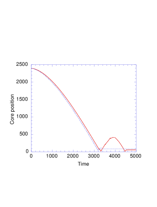
  Figure 2: Core position of collapsing loop versus time for $\lambda=0.001$ (dotted line) and $\lambda=0.004$ (solid line). The lattice size is $4096\times 4096$.

  and then time-evolved using the finite difference equations which follow from Eq. (26). FFT spectrum analysis of the kinetic and gradient energies during the collapse yields $N_{ax}(t)$.

  3.1 Computer simulations of circular loops

  Because of azimuthal symmetry, circular loops can be studied in $r-z$ space. By mirror symmetry, the problem can be further reduced to one quarter-plane. The static axion field far from the string core is

  $$a(r,z)=\frac{f_{a}}{2}\Omega(r,z)$$ (39)

  in the infinite volume limit, where $\Omega$ is the solid angle subtended by the loop. We use as initial configuration the outcome of a relaxation routine starting with Eq. (39) outside the core and $\phi(\rho)\approx 0.58(\rho/\delta)\exp(i\theta)$ within the core. Here, $\rho$ is the distance to the string, and $\theta$ is the winding angle. The relaxation and the subsequent dynamical evolution are done with reflective boundary conditions. A step size $dt$ = 0.2 was used for the time evolution and the total energy was conserved to better than 1 %.

  

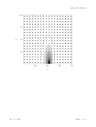
  Figure 4: Intensity plot of potential energy (contours represent constant potential energy) in vicinity of string core for $R_{0}=2400,\lambda=0.001$ at $t=2600$. The Lorentz factor is about 4. The arrows represent the axion field.

  In general the loops collapsed at nearly the speed of light without a rebound. For a small range of parameters, $80<R_{0}/\delta<190$, where $R_{0}$ is the initial loop radius, we noticed a small bounce as show in Figure 1. There is a substantial Lorentz contraction of the string core as it collapses (see Figure 2). A lattice effect became evident when the reduced core size becomes comparable to the lattice spacing. This consists of a “scraping” of the string core on the underlying grid, during which the kinetic energy of the string gets dissipated into high frequency axion radiation. We always choose $\lambda$ small enough to avoid this phenomenon.

  Spectrum analysis of the fields was performed by expanding the gradient and kinetic energies as

  $$\nabla_{z}\phi=\sum_{mn}c_{mn}J_{0}(k_{m}r)\,\sin(k_{n}z)$$

  $$\nabla_{r}\phi=\sum_{mn}c_{mn}J_{1}(k_{m}r)\,\cos(k_{n}z)$$

  $$\dot{\phi}=\sum_{mn}c_{mn}J_{0}(k_{m}r)\,\cos(k_{n}z)$$ (40)

  with the boundary conditions $J_{1}(k_{m}R_{\rm max})=0$ and ${\rm sin}(k_{n}Z_{\rm max})=0$. The dispersion relationship for axions is given by $\omega_{mn}=\sqrt{k_{m}^{2}+k_{n}^{2}}$. Figure 3 shows the power spectrum $dE/d\ln k$ displayed in ${\rm ln}k$ bins of width $\Delta\ln k=0.5$, at $t=0$ and after the collapse at $t=3000$. At both times, the spectrum

  

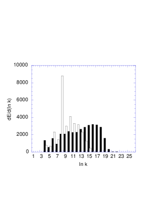
  Figure 6: Energy spectrum of collapsing loop for $R_{0}=2400$ and $\lambda=0.001$. The white (black) histogram represents the spectrum at $t=0(t=3000).$ The increased high frequency cutoff of the final spectrum is due to the Lorentz contraction of the core.

  exhibits an almost flat plateau, consistent with $dE/dk\propto 1/k$. The high frequency cutoff of the spectrum is increased however after the collapse and is associated with the Lorentz contraction of the core. The evolution of $N_{ax}=\sum_{mn}(E_{mn}/k_{mn})$ during the loop

  

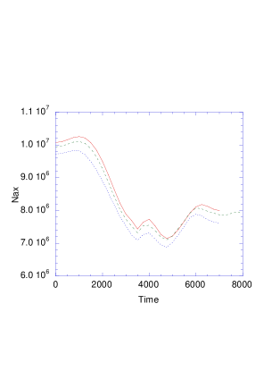
  Figure 8: $N_{ax}$ of a circular loop as a function of time for $R_{0}=2400$, and $\lambda=0.004$ (solid line), $\lambda=0.001$ (dashed line), and $\lambda=0.00025$ (dotted line).

  collapse was studied for various values of $R_{0}/\delta$. We observe a marked decrease of $N_{ax}$ by $\sim 20\%$ during the collapse roughly independent of $R_{0}/\delta$.

  3.2 Computer simulations of rotating loops

  There exists a family of nonintersecting (“Kibble-Turok”) loops [22, 23, 24], which have been studied in the context of gauge strings. They are solutions of the Nambu-Goto equations of motion and have non-zero angular momentum. Intercommuting (self-intersection with reconnection) causes the loop sizes to shrink, and hence the average energy of radiated axions to increase and hence $N_{ax}$ to decrease. Intercommuting favors scenario B for these reasons. We picked the Kibble-Turok configuration as an initial condition to avoid intercommuting as much as possible and give scenario A the best possible chance to get realized. A common loop parametrization is given by [23]

  $$x(\sigma,t) = \frac{R}{2}\left((1-\alpha)\,\sin\sigma_{-}+\frac{1}{3}\alpha\,\sin 3\sigma_{-}+\sin\sigma_{+}\right)$$

  $$y(\sigma,t) = \frac{R}{2}\left(-(1-\alpha)\,\cos\sigma_{-}-\frac{1}{3}\alpha\,\sin 3\sigma_{-}-\cos\psi\,\cos\sigma_{+}\right)$$

  $$z(\sigma,t) = \frac{R}{2}\left(-2\sqrt{\alpha(1-\alpha)}\,\cos\sigma_{-}-\sin\psi\,\cos\sigma_{+}\right)$$ (41)

  where $\sigma_{\pm}=(\sigma\pm t)/R$, and $\sigma\in(0,2\pi R)$ is the length along the loop. For a significant subset of the free parameters $\alpha\in(0,1)$, $\psi\in(-\pi,\pi)$, the loop never self-intersects. A noteworthy feature in the case of gauge strings is the periodic appearance of cusps, where the string velocity momentarily reaches the speed of light.

  We performed numerous simulations of rotating loops on a 3D $(256^{3})$ lattice with periodic boundary conditions. Standard Fourier techniques were used

  

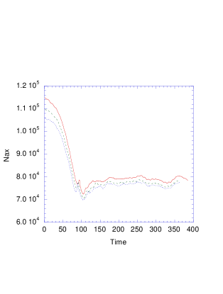
  Figure 10: $N_{ax}$ of non-intersecting (”Kibble-Turok”) loops as a function of time for $\alpha=0.01,\phi=0$, and $\lambda=0.2$ (solid line), $\lambda=0.1$ (dashed line), and $\lambda=0.0625$ (dotted line). The lattice size is $256^{3}$ and $R=72$.

  for the spectrum analysis, and $N_{ax}$ was computed as a function of time using the dispersion relationship

  $$\omega_{mnp}=\sqrt{2(3-\cos k_{m}-\cos k_{n}-\cos k_{p})}$$ (42)

  Figure 5 shows $N_{ax}$ for various core sizes and constant $\alpha,\psi$. The behavior is very similar to that of a non-rotating circular loop with a

  

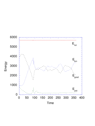
  Figure 12: Energy of non-intersecting loop. Shown are total, gradient, kinetic, and potential energy as a function of time for $\alpha=0.01,\psi=0$, and $\lambda=0.0625$.

  reduction of $N_{ax}$ of about $25\%$. Figure 6 depicts the energy of the collapsing loop. Clearly, the total energy is well conserved. A few percent of the loop energy is dissipated as massive radiation, shown here as $E_{\rm pot}$.

  3.3 Conclusions

  In our 3D simulations of rotating loops, $r\simeq 0.75$ for $\ln(L/\delta)\simeq 4$. We take $L=2R$. In our 2D simulations of circular loops, $r\simeq 0.8$ for $\ln(L/\delta)\simeq 6$. The earlier 3D simulations of circular loops by two of us found $r\simeq 0.8$ for $\ln(L/\delta)\simeq 4$. We conclude that $r$ is of order one when $\ln(L/\delta)\simeq 6$, and that $r$ does not appear to change when $\ln(L/\delta)$ is increased. Hence we find the string decay contribution to the axion cosmological energy density Eq. (38)] to be of the same order of magnitude as that from vacuum realignment [Eqs. (23,25)].

  4 Wall decay

  During the QCD phase transition, when the axion acquires mass, each axion string becomes the boundary of $N$ domain walls. If $N>1$ there is a domain wall problem as mentioned in the introduction. We assume $N=1$ here. Each string is therefore attached to one domain wall. The domain walls bounded by string are like pancakes or long surfaces with holes. A simple statistical argument [11] shows that domain walls which are not bounded by string, and therefore close onto themselves like spheres or donuts, are very rare.

  When the axion acquires mass, the model of Eq. (26) gets modified as follows:

  $${\cal L}=\frac{1}{2}\partial_{\mu}\phi_{1}\partial^{\mu}\phi_{1}+\frac{1}{2}\partial_{\mu}\phi_{2}\partial^{\mu}\phi_{2}-\frac{\lambda}{4}(\phi_{1}^{2}+\phi_{2}^{2}-v_{a}^{2})^{2}+\eta v_{a}\phi_{1}$$ (43)

  The axion mass $m_{a}=\sqrt{\eta}$ for $v_{a}\gg m_{a}$. We may set $\phi(x)=v_{a}e^{\frac{i}{v_{a}}a(x)}$ when restricting ourselves to low energy configurations. The corresponding effective Lagrangian is :

  $${\cal L}_{a}=\frac{1}{2}\partial_{\mu}a\partial^{\mu}a+m_{a}^{2}v_{a}^{2}\left[\cos\left(\frac{a}{v_{a}}\right)-1\right].$$ (44)

  Its equation of motion has the well-known Sine-Gordon soliton solution :

  $$\frac{a(y)}{v_{a}}=2\pi n+4\tan^{-1}\exp(m_{a}y)$$ (45)

  where $y$ is the coordinate perpendicular to the wall and $n$ is any integer. Eq. (45) describes a domain wall which interpolates between neighboring vacua in the low energy effective theory (44). In the original theory (43), the domain wall interpolates between the unique vacuum back to that same vacuum going around the bottom of the Mexican hat potential $V(\phi^{\dagger}\phi)=\frac{\lambda}{4}(\phi^{\dagger}\phi-v_{a}^{2})^{2}$ once.

  The thickness of the wall is of order $m_{a}^{-1}$. The wall energy per unit surface is $\sigma=8m_{a}v_{a}^{2}$ in the toy model of Eq. (43). In reality the structure of axion domain walls is more complicated than in the toy model, because not only the axion field but also the neutral pion field is spatially varying inside the wall [25]. When this is taken into account, the (zero temperature) wall energy/surface is found to be:

  $$\sigma\simeq 4.2~{}f_{\pi}m_{\pi}f_{a}\simeq 9~{}m_{a}f_{a}^{2}\$$ (46)

  with $f_{a}\equiv v_{a}/N$. For $N=1$, $f_{a}$ and $v_{a}$ are the same. However, written in terms of $f_{a}$, Eq. (46) is valid for $N\neq 1$ also.

  Walls bounded by strings are of course topologically unstable. In ref.[11] we discussed three decay mechanisms - emission of gravitational waves, friction on the surrounding plasma and emission of axions - and concluded that decay into non-relativistic axions is very likely the dominant mechanism. This is consistent with the computer simulations described below. In the simulations the walls decay immediately, i.e. in a time of order their size divided by the speed of light, and the average energy of the radiated axions is $\langle\omega_{a}\rangle\sim 7m_{a}$.

  Let $t_{3}$ be the time when the decay effectively takes place in the early universe and let $\gamma\equiv\frac{\langle\omega_{a}\rangle}{m_{a}(t_{3})}$ be the average Lorentz $\gamma$ factor then of the axions produced. The density of walls at time $t_{1}$ was estimated [11] to be of order $0.7$ per horizon volume. Hence the average energy density in walls between $t_{1}$ and $t_{3}$ is of order

  $$\rho_{\rm d.w.}(t)\sim(0.7)(9)m_{a}(t)\frac{f_{a}^{2}}{t_{1}}\left(\frac{R_{1}}{R}\right)^{3}\,.$$ (47)

  We used Eq. (46) and assumed that the energy in walls simply scales as $m_{a}(t)$. After time $t_{3}$, the number density of axions produced in the decay of walls bounded by strings is of order

  $$n^{\rm d.w.}_{a}(t)\sim\frac{\rho_{\rm d.w.}(t_{3})}{\langle\omega_{a}\rangle}\left(\frac{R_{3}}{R}\right)^{3}\sim\frac{6}{\gamma}\frac{f_{a}^{2}}{t_{1}}\left(\frac{R_{1}}{R}\right)^{3}\,.$$ (48)

  Note that the dependence on $t_{3}$ drops out of our estimate of $n^{\rm d.w.}_{a}$.

  4.1 Computer simulations

  

  Figure 14: Speed of the string core as a function of time for the case $1/m_{a}=400$, $\sqrt{\lambda}/m_{a}=10$, and $v=0$.

  We have carried out an extensive program of 2D numerical simulations of domain walls bounded by strings using the Lagrangian of Eq. (43) in finite difference form. We report our results in units where $v_{a}=1$ and the lattice constant is the unit of length. Thus the wall thickness is $1/m_{a}=1/\sqrt{\eta}$ and the core size is $\delta=1/\sqrt{\lambda}$. In the continuum limit, the dynamics depends upon a single critical parameter, $m_{a}\delta=m_{a}/\sqrt{\lambda}$. Large two-dimensional grids $(\sim 4000\times 4000)$ were initialized with a straight domain wall initially at rest or with angular momentum. The initial domain wall was obtained by overrelaxation starting with the Sine-Gordon ansatz $\phi_{1}+i\phi_{2}={\rm exp}(i\,{\rm tan^{-1}exp}(m_{a}y))$ inside a strip of length $D$ between the string and anti-string and the true vacuum $(\phi_{1}=1,\,\phi_{2}=0)$ outside. The string and anti-string core were approximated by $\phi_{1}+i\phi_{2}=-{\rm tanh}(.583\,r/\delta)\,{\rm exp}(\mp i\theta)$ where $(r,\theta)$ are polar coordinates about the core center, and held fixed during relaxation. Stable domain walls were obtained for $1/(\delta m_{a})\mathrel{\raise 1.29167pt\hbox{$>$\kern-7.5pt\lower 4.30554pt\hbox{$\sim$}}}3$. A first-order in time and second order in space algorithm was used for evolution with a time step $dt=0.2$. The boundary conditions were periodic and the total energy was conserved to better than 1%. If the angular momentum was nonzero, the initial time derivative $\dot{\phi}$ was obtained by a finite difference over a small time step.

  

  Figure 16: Position of the string or anti-string core as a function of time for $1/m_{a}=1000$, $\lambda=0.0002,D=2896$, and $v=0$. The string and anti-string cores have opposite $z$. They go through each other and oscillate with decreasing amplitude.

  The evolution of the domain wall was studied for various values of $\sqrt{\lambda}/m_{a}$, the initial wall length $D$ and the initial velocity $v$ of the strings in the direction transverse to the wall. Fig. 14 shows the longitudinal velocity of the core as a function of time for the case $m_{a}^{-1}=400,\sqrt{\lambda}/m_{a}=10$ and $v=0$. An important feature is the Lorentz contraction of the core. For reduced core sizes $\delta/\gamma_{s}\mathrel{\raise 1.29167pt\hbox{$<$\kern-7.5pt\lower 4.30554pt\hbox{$\sim$}}}5$, where $\gamma_{s}$ is the Lorentz factor associated with the speed of the string core, there is ’scraping’ of the core on the lattice accompanied by emission of spurious high frequency radiation. This artificial friction eventually balances the wall tension and leads to a terminal velocity. In our simulations we always ensured being in the continuum limit.

  

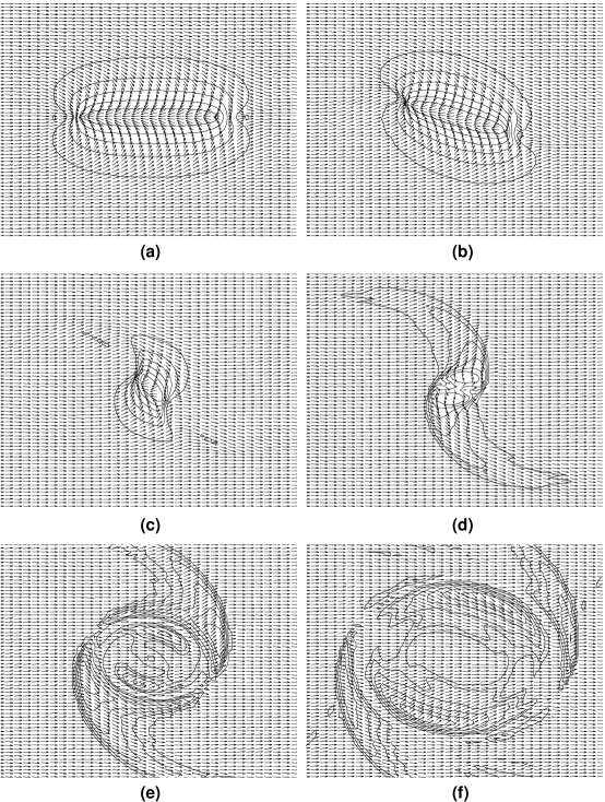
  Figure 18: Decay of a wall at successive time intervals $\Delta t=1.2/m_{a}$ for the case $m_{a}^{-1}=100$, $\lambda=0.01$, $D=524$, and $v=0.6$.

  For a domain wall without rotation ($v=0$), the string cores strike head-on and go through each other. Several oscillations of decreasing magnitude generally occur before annihilation. For $\gamma_{s}\simeq 1$ the string and anti-string coalesce and annihilate one another. For $\gamma_{s}\mathrel{\raise 1.29167pt\hbox{$>$\kern-7.5pt\lower 4.30554pt\hbox{$\sim$}}}2$, the strings go through each other and regenerate another wall of reduced length. The relative oscillation amplitude decreases with decreasing collision velocity. Fig. 16 shows the core position as a function of time for the case $m_{a}^{-1}=1000,\sqrt{\lambda}/m_{a}=14.3,D=2896$.

  We also investigated the more generic case of a domain wall with angular momentum. The strings are similarly accelerated by the wall but string and anti-string cores miss each other. The field is displayed in Fig. 18 at six time steps for the case $m_{a}^{-1}=100,\lambda=0.01,D=524$ and $v=0.6$. No oscillation is observed. All energy is converted into axion radiation during a single collapse.

  

  Figure 20: Energy spectrum at successive time intervals $\Delta t=1/m_{a}$, with $w_{\rm max}=\sqrt{8+m_{a}^{2}}$ and $l_{W}=18\ln(w/m_{a})/\ln(w_{\rm max}/m_{a})$ $+2$, for the case $m_{a}^{-1}=500$, $\lambda=0.0032$, $D=2096$ and $v=0.25$.

  We performed spectrum analysis of the energy stored in the $\phi$ field as a function of time using standard Fourier techniques. The two-dimensional Fourier transform is defined by

  $$\tilde{f}(\vec{p})\!=\!\frac{1}{\sqrt{V}}\!\sum_{\vec{n}}\!\exp\!\left[2i\pi\left(\frac{p_{x}n_{x}}{L_{x}}+\frac{p_{y}n_{y}}{L_{y}}\right)\right]\!f(\vec{n})$$ (49)

  where $V\equiv L_{x}L_{y}$. The dispersion law is:

  $$\omega_{p}=\sqrt{2\left(2-\cos\frac{2\pi p_{x}}{L_{x}}-\cos\frac{2\pi p_{y}}{L_{y}}\right)+m_{a}^{2}}.$$ (50)

  Fig. 20 shows the power spectrum $dE/d\ln\omega$ of the $\phi$ field at various times during the decay of a rotating domain wall for the case $m_{a}^{-1}=500,\lambda=0.0032,D=2096$, and $v=0.25$. Initially, the spectrum is dominated by small wavevectors, $k\sim m_{a}$. Such a spectrum is characteristic of the domain wall. As the wall accelerates the string, the spectrum hardens until it becomes roughly $1/k$ with a long wavelength cutoff of order the wall thickness $1/m_{a}$ and a short wavelength cutoff of order the reduced core size $\delta/\gamma_{s}$. Such a spectrum is characteristic of the moving string.

  

  Figure 22: $\langle\omega\rangle$ as a function of time for $1/m_{a}=500$, $D=2096$, $v=0.25$ and $\lambda=$ 0.0004 (solid), 0.0008 (long dash), 0.0016 (short dash), 0.0032 (dot) and 0.0064 (dot dash). After the wall has decayed, $\langle\omega\rangle$ is the average energy of radiated axions.

  Fig. 22 shows the time evolution of $\langle\omega\rangle/m_{a}$ for $m_{a}^{-1}=500,v=0.25,D=2096$ and various values of $\lambda$. By definition,

  $$\langle\omega\rangle=\sum_{\vec{p}}E_{\vec{p}}/\sum_{\vec{p}}\frac{E_{\vec{p}}}{\omega_{\vec{p}}}$$ (51)

  where $E_{\vec{p}}$ is the gradient and kinetic energy stored in mode $\vec{p}$ of the field $\phi$. After the domain wall has decayed into axions, $\langle\omega\rangle=\langle\omega_{a}\rangle$. Fig. 24 shows the time evolution of $\langle\omega\rangle/m_{a}$ for $m_{a}^{-1}=500,\lambda=0.0016,D=2096$ and various values of $v$.

  

  Figure 24: Same as in Fig. 22 except $\lambda=0.0016$, and $v=$ 0.15 (solid), 0.25 (long dash), 0.4 (short dash) and 0.6 (dot).

  When the angular momentum is low and the core size is big, the strings have one or more oscillations. In that case, $\langle\omega_{a}\rangle/m_{a}\simeq 4$, which is consistent with Ref. [16]. We believe this regime to be less relevant to wall decay in the early universe because it seems unlikely that the angular momentum of a wall at the QCD epoch could be small enough for the strings to oscillate.

  In the more generic case when no oscillations occur, $\langle\omega_{a}\rangle/m_{a}\simeq 7$. Moreover, we find that $\langle\omega_{a}\rangle/m_{a}$ depends upon the critical parameter $\sqrt{\lambda}/m_{a}$, increasing approximately as the logarithm of that quantity; see Fig. 22. This is consistent with the time evolution of the energy spectrum, described in Fig. 10. For a domain wall, $\langle\omega\rangle\sim m_{a}$ whereas for a moving string $\langle\omega\rangle\sim m_{a}\ln(\sqrt{\lambda}v_{a}\gamma_{s}/m_{a})$. Since we find the decay to proceed in two steps: 1) the wall energy is converted into string kinetic energy, and 2) the strings annihilate without qualitative change in the spectrum, the average energy of radiated axions is $\langle\omega_{a}\rangle\sim m_{a}\ln(\sqrt{\lambda}v_{a}/m_{a})$. Assuming this is a correct description of the decay process for $\sqrt{\lambda}v_{a}/m_{a}\sim 10^{26}$, then $\langle\omega_{a}\rangle/m_{a}\sim 60$ in axion models of interest.

  4.2 Conclusions

  If we use the value $\gamma=7$ observed in our computer simulations, Eq. (48) becomes

  $$n^{\rm d.w.}_{a}(t)\sim\frac{f_{a}^{2}}{t_{1}}\left(\frac{R_{1}}{R}\right)^{3}\,.$$ (52)

  In that case the contributions from vacuum realignment [Eq. (23) and Eq. (25)] and domain wall decay are of the same order of magnitude. However, we find that $\gamma$ rises approximately linearly with ln$(\sqrt{\lambda}v_{a}/m_{a})$ over the range of ln$(\sqrt{\lambda}v_{a}/m_{a})$ investigated in our numerical simulations. If this behaviour is extrapolated all the way to ln$(\sqrt{\lambda}v_{a}/m_{a})\simeq 60$, which is the value in axion models of interest, then $\gamma\simeq 60$. In that case the contribution from wall decay is subdominant relative to that from vacuum realignment.

  5 The cold axion cosmological energy density

  For case 1, adding the three contributions, we estimate the present cosmological energy density in cold axions to be:

  $$\rho_{a}(t_{0})\sim 3{f_{a}^{2}\over t_{1}}\left({R_{1}\over R_{0}}\right)^{3}m_{a}~{}~{}~{}~{}~{}~{}~{}~{}~{}(case~{}1)\ .$$ (53)

  Following [6], we may determine the ratio of scale factors $R_{1}/R_{0}$ by assuming the conservation of entropy from time $t_{1}$ till the present. The number of effective thermal degrees of freedom at time $t_{1}$ is approximately ${\cal N}_{1}\simeq 61.75$. We do not include axions in this number because they are decoupled by then. Let $t_{4}$ be a time (say $T_{4}=4$ MeV) after the pions and muons annihilated but before neutrinos decoupled. The number of effective thermal degrees of freedom at time $t_{4}$ is ${\cal N}_{4}=10.75$ with electrons, photons and three species of neutrinos contributing. Conservation of entropy implies ${\cal N}_{1}T_{1}^{3}R_{1}^{3}={\cal N}_{4}T_{4}^{3}R_{4}^{3}$. The neutrinos decouple before $e^{+}e^{-}$ annihilation. Therefore, as is well known, the present temperature $T_{\gamma 0}=2.735~{}^{0}$K of the cosmic microwave background is related to $T_{4}$ by: ${11\over 2}T_{4}^{3}R_{4}^{3}=2~{}T_{0\gamma}^{3}~{}R_{0}^{3}$. Putting everything together we have

  $$\left({R_{1}\over R_{0}}\right)^{3}\simeq 0.063\left({T_{\gamma,0}\over T_{1}}\right)^{3}\ .$$ (54)

  Combining Eqs. (19), (53) and (54),

  $$\rho_{a}(t_{0})\sim 10^{-29}{\mbox{gr}\over\mbox{cm}^{3}}\left({f_{a}\over 10^{12}\mbox{GeV}}\right)^{7/6}~{}~{}~{}~{}~{}(case~{}1)\ .$$ (55)

  Dividing by the critical density $\rho_{c}={3H_{0}^{2}\over 8\pi G}$, we find:

  $$\Omega_{a}\sim\left({f_{a}\over 10^{12}\mbox{GeV}}\right)^{7/6}\left({0.7\over h}\right)^{2}~{}~{}~{}~{}~{}~{}~{}~{}~{}~{}(case~{}1)$$ (56)

  where $h$ is defined as usual by $H_{0}=h~{}100$km/s$\cdot$Mpc.

  For case 2, we have

  $$\Omega_{a}\sim{1\over 6}\left({f_{a}\over 10^{12}\mbox{GeV}}\right)^{7/6}\left({0.7\over h}\right)^{2}\alpha^{2}(t_{1})~{}~{}~{}~{}~{}~{}~{}~{}(case~{}2)$$ (57)

  where $\alpha(t_{1})$ is the unknown misalignment angle.

  6 Pop. I and Pop. II axions

  On the basis of the discussion in sections 2 to 4 we distinguish two kinds of cold axions:
  

  I) axions which were produced by vacuum realignment or string decay and which were not hit by moving domain walls. They have typical momentum $\langle p_{I}(t_{1})\rangle\sim\frac{1}{t_{1}}$ at time $t_{1}$ because they are associated with axion field configurations which are inhomogeneous on the horizon scale at that time. Their velocity dispersion is of order:

  $$\beta_{I}(t)\sim\frac{1}{m_{a}t_{1}}\left(\frac{R_{1}}{R}\right)\simeq 3\cdot 10^{-17}\left(\frac{10^{-5}{\rm eV}}{m_{a}}\right)^{5/6}\frac{R_{0}}{R}\ .$$ (58)

  We call these axions population I.
  

  II) axions which were produced in the decay of domain walls. They have typical momentum $\langle p_{II}(t_{3})\rangle\sim\gamma m_{a}(t_{3})$ at time $t_{3}$ when the walls effectively decay. Their velocity dispersion is of order:

  $$\beta_{II}(t)\sim\gamma\frac{m_{a}(t_{3})}{m_{a}}\frac{R_{3}}{R}\simeq 10^{-13}\left(\ \gamma\frac{m_{a}(t_{3})}{m_{a}}\frac{R_{3}}{R_{1}}\right)\left(\frac{10^{-5}{\rm eV}}{m_{a}}\right)^{1/6}\frac{R_{0}}{R}\,.$$ (59)

  The factor $q\equiv\gamma\frac{m_{a}(t_{3})}{m_{a}}\frac{R_{3}}{R_{1}}$ parametrizes our ignorance of the wall decay process. We expect $q$ to be of order one but with very large uncertainties. There is however a lower bound [11]: $q\mathrel{\raise 1.29167pt\hbox{$>$\kern-7.5pt\lower 4.30554pt\hbox{$\sim$}}}\frac{\gamma}{130}\left(\frac{10^{-5}{\rm eV}}{m_{a}}\right)^{2/3}$. Since our computer simulations suggest $\gamma$ is in the range 7 to 60, the axions of the second population (pop. II) have much larger velocity dispersion than the pop. I axions.
  

  Note that there are axions which were produced by vacuum realignment or string decay but were hit by relativistically moving walls at some time between $t_{1}$ and $t_{3}$. These axions are relativistic just after getting hit and therefore are part of pop. II rather than pop. I.

  The fact that there are two populations of cold axions, with widely differing velocity dispersion, has interesting implications for the formation and evolution of axion miniclusters [26, 27]. We showed [11] that the QCD horizon scale density perturbations in pop. II axions get erased by free streaming before the time $t_{eq}$ of equality between radiation and matter whereas those in pop. I axions do not. Hence, whereas pop. I axions form miniclusters, pop. II axions form an unclustered component of the axion cosmological energy density which guarantees that the signal in direct searches for axion dark matter is on all the time.

  The primordial velocity dispersion of pop. II axions may some day be measured in a cavity-type axion dark matter detector [28]. If a signal is found in such a detector, the energy spectrum of dark matter axions will be measured with great resolution. It has been pointed out that there are peaks in the spectrum [29] because late infall produces distinct flows, each with a characteristic local velocity vector. These peaks are broadened by the primordial velocity dispersion, given in Eqs. (58) and (59) for pop. I and pop. II axions respectively. These equations give the velocity dispersion in intergalactic space. When the axions fall onto the galaxy their density increases by a factor of order $10^{3}$ and hence, by Liouville’s theorem, their velocity dispersion increases by a factor of order 10. [Note that this increase is not isotropic in velocity space. Typically the velocity dispersion is reduced in the direction longitudinal to the flow in the rest frame of the galaxy whereas it is increased in the two transverse directions.] The energy dispersion measured on Earth is $\Delta E=m_{a}\beta\Delta\beta$ where $\beta\simeq 10^{-3}$ is the flow velocity in the rest frame of the Earth. Hence we find $\Delta E_{I}\sim 3\cdot 10^{-19}\left(\frac{10^{-5}{\rm eV}}{m_{a}}\right)^{5/6}m_{a}$ for pop. I axions and $\Delta E_{II}\sim 10^{-15}~{}q~{}\left(\frac{10^{-5}{\rm eV}}{m_{a}}\right)^{1/6}m_{a}$ for pop. II. The minimum time required to measure $\Delta E$ is $(\Delta E)^{-1}$. This assumes ideal measurements and also that all sources of jitter in the signal not due to primordial velocity dispersion can be understood. There is little hope of measuring the primordial velocity dispersion of pop. I axions since $(\Delta E_{I})^{-1}\sim 10~{}{\rm years}\left(\frac{10^{-5}{\rm eV}}{m_{a}}\right)^{1/6}$. However $(\Delta E_{II})^{-1}\sim~{}$day $q^{-1}\left(\frac{10^{-5}{\rm eV}}{m_{a}}\right)^{5/6}$, and hence it is conceivable that the primordial velocity dispersion of pop. II axions will be measured.

  Acknowledgements

  This research was supported in part by DOE grant DE-FG05-86ER40272 at the University of Florida and by DOE grant W-7405-ENG-048 at Lawrence Livermore National Laboratory.

References

- [1] R. D. Peccei and H. Quinn, Phys. Rev. Lett. 38, 1440 (1977); Phys. Rev. D16, 1791 (1977); S. Weinberg, Phys. Rev. Lett. 40, 223 (1978); F. Wilczek, Phys. Rev. Lett. 40, 279 (1978).
- [2] J. E. Kim, Phys. Rep. 150, 1 (1987); H.-Y. Cheng, Phys. Rep. 158, 1 (1988); R. D. Peccei, in CP Violation, Ed. by C. Jarlskog, World Scientific Publ., 1989, pp 503-551; M. S. Turner, Phys. Rep. 197, 67 (1990); G. G. Raffelt, Phys. Rep. 198, 1 (1990).
- [3] P. Sikivie, Phys. Rev. Lett. 48, 1156 (1982).
- [4] H.-T. Janka, W. Keil, G. Raffelt and D. Seckel, Phys. Rev. Lett. 76, 2621 (1996); W. Keil, H.-T. Janka, D.N. Schramm, G. Sigl, M.S. Turner and J. Ellis, Phys. Rev. D56, 2419 (1997).
- [5] D. J. Gross R. D. Pisarski and L. G. Yaffe, Rev. Mod. Phys. 53, 43 (1981).
- [6] L. Abbot and P. Sikivie, Phys. Lett. B120, 133 (1983); J. Preskill, M. Wise and F. Wilczek, Phys. Lett. B120, 127 (1983); M. Dine and W. Fischler, Phys. Lett. 120, 137 (1983).
- [7] R. Davis, Phys. Rev. D32, 3172 (1985); Phys. Lett. B180, 225 (1986).
- [8] D. Harari and P. Sikivie, Phys. Lett. B195, 361 (1987).
- [9] A. Vilenkin and A.E. Everett, Phys. Rev. Lett. 48, 1867 (1982).
- [10] P. Sikivie in Where are the elementary particles, Proc. of the 14th Summer School on Particle Physics, Gif-sur-Yvette, 1982, edited by P. Fayet et al. (Inst. Nat. Phys. Nucl. Phys. Particules, Paris, 1983).
- [11] S. Chang, C. Hagmann and P. Sikivie, hep-ph/9807374, to appear in Phys. Rev. D.
- [12] A. Vilenkin and T. Vachaspati, Phys. Rev. D35, 1138 (1987); R.L. Davis and E.P.S. Shellard, Nucl. Phys. B324, 167 (1989); A. Dabholkar and J.M. Quashnock, Nucl. Phys. B333, 815 (1990); R.A. Battye and E.P.S. Shellard, Nucl. Phys. B423, 260 (1994); Phys. Rev. Lett. 73, 2954 (1994); (E) ibid. 76, 2203 (1996); astro-ph/9802216; M. Yamaguchi, M. Kawasaki and J. Yokoyama, hep-ph/ 9811311.
- [13] C. Hagmann and P. Sikivie, Nucl. Phys. B363, 247 (1991);
- [14] C. Hagmann, S. Chang and P. Sikivie, hep-ph/9807428.
- [15] D. H. Lyth, Phys. Lett. B275, 279 (1992).
- [16] M. Nagasawa and M. Kawasaki, Phys. Rev. D50, 4821 (1994).
- [17] E.W. Kolb and M.S. Turner, The Early Universe, Addison-Wesley, 1990.
- [18] P. J. Steinhardt and M. S. Turner, Phys. Lett. B129, 51 (1983); W. G. Unruh and R. M. Wald, Phys. Rev. D32, 831 (1985); M. S. Turner, Phys. Rev. D32, 843 (1985); T. DeGrand, T. W. Kephart and T. J. Weiler, Phys. Rev. D33, 910 (1986); G. Lazarides, R. Schaefer, D. Seckel and Q. Shafi, Nucl. Phys. B346, 193 (1990); M. Hindmarsh, Phys. Rev. D45, 1130 (1992).
- [19] C. T. Hill and G. G. Ross, Nucl. Phys. B311, 253 (1988).
- [20] E.W. Kolb, A. Singh and M. Srednicki, hep-ph/9709285; P.B. Greene, L. Kofman and A.A. Starobinsky, hep-ph/9808477.
- [21] A. D. Linde, JETP Lett. 40 (1984) 1333 and Phys. Lett. B158 (1985) 375; D. Seckel and M. Turner, Phys. Rev. D32 (1985) 3178; D. H. Lyth, Phys. Lett. B236 (1990) 408; A. D. Linde and D. H. Lyth, Phys. Lett. B246 (1990) 353; M. Turner and F. Wilczek, Phys. Rev. Lett. 66 (1991) 5; A. Linde, Phys. Lett. B259 (1991) 38; D.H. Lyth, Phys. Rev. D45 (1992) 3394; D.H. Lyth and E.D. Stewart, Phys. Lett. B283 (1992) 189 and Phys. Rev. D46 (1992) 532.
- [22] T.W.B. Kibble and N. Turok, Phys. Lett. 116B, 141 (1982).
- [23] N. Turok, Nucl. Phys. B242, 520 (1984).
- [24] C. Burden, Phys. Lett. 164B, 277 (1985); A.L. Chen, D.A. DiCarlo, and S.A. Hotes, Phys. Rev. D37, 863 (1988).
- [25] M.C. Huang and P. Sikivie, Phys. Rev. 32, 1560 (1985).
- [26] C. J. Hogan and M. J. Rees, Phys. Lett. B205, 228 (1988).
- [27] E. W. Kolb and I. Tkachev, Phys. Rev. Lett. 71, 3051 (1993).
- [28] P. Sikivie, Phys. Rev. Lett. 51, 1415 (1983) and Phys. Rev. D32, 2988 (1985); L. Krauss et al., Phys.Rev. Lett. 55, 1797 (1985); S. DePanfilis et al., Phys. Rev. Lett. 59, 839 (1987) and Phys. Rev. D40, 3151 (1989); C. Hagmann et al., Phys. Rev. D42, 1297 (1990); K. van Bibber et al., Int. J. Mod. Phys. D3 Suppl. 33 (1994); S. Matsuki et al., Phys. Lett. 336, 573 (1994); C. Hagmann et al, Phys. Rev. Lett. 80, 2043 (1998).
- [29] P. Sikivie and J. Ipser, Phys. Lett. B291, 288 (1992); P. Sikivie, I. Tkachev and Y. Wang, Phys. Rev. Lett. 75, 2911 (1995) and Phys. Rev. D 56, 1863 (1997).