ABSTRACT

These lectures provide an introduction to the basic aspects of the Standard Model, $SU(3)_{C}\times SU(2)_{L}\times U(1)_{Y}$.

1 Introduction

All known particle physics phenomena are extremely well described within the Santard Model (SM) of elementary particles and their fundamental interactions. The SM provides a very elegant theoretical framework and it has succesfully passed very precise tests which at present are at the $0.1\%$ level [1, 2, 3, 4].

We understand by elementary particles the point-like constituents of matter with no known substructure up to the present limits of $10^{-18}-10^{-19}m$. These are of two types, the basic building blocks of matter themselves konwn as matter particles and the intermediate interaction particles. The first ones are fermions of spin $s=\frac{1}{2}$ and are classified into leptons and quarks. The known leptons are: the electron, $e^{-}$, the muon, $\mu^{-}$ and the $\tau^{-}$ with electric charge $Q=-1$ (all charges are given in units of the elementary charge $e$); and the corresponding neutrinos $\nu_{e}$, $\nu_{\mu}$ and $\nu_{\tau}$ with $Q=0$. The known quarks are of six different flavors: $u$, $d$, $s$, $c$, $b$ and $t$ and have fractional charge $Q=$ $\frac{2}{3}$,$-\frac{1}{3}$, $-\frac{1}{3}$, $\frac{2}{3}$, $-\frac{1}{3}$ and $\frac{2}{3}$ respectively.

The quarks have an additional quantum number, the color, which for them can be of three types, generically denoted as $q_{i}$, $i=1,2,3$. We know that color is not seen in Nature and therefore the elementary quarks must be confined into the experimentally observed matter particles, the hadrons. These colorless composite particles are classified into baryons and mesons. The baryons are fermions made of three quarks, $qqq$, as for instance the proton, $p\sim uud$, and the neutron, $n\sim ddu$. The mesons are bosons made of one quark and one antiquark as for instance the pions, $\pi^{+}\sim u{\bar{d}}$ and $\pi^{-}\sim d{\bar{u}}$.

The second kind of elementary particles are the intermediate interaction particles. By leaving apart the gravitational interactions, all the relevant interactions in Particle Physics are known to be mediated by the exchange of an elementary particle that is a boson with spin $s=1$. The photon, $\gamma$, is the exchanged particle in the electromagnetic interactions, the eight gluons $g_{\alpha}\;;\alpha=1,..8$ mediate the strong interactions among quarks, and the three weak bosons, $W^{\pm}$, $Z$ are the corresponding intermediate bosons of the weak interactions.

As for the theoretical aspects, the SM is a quantum field theory that is based on the gauge symmetry $SU(3)_{C}\times SU(2)_{L}\times U(1)_{Y}$. This gauge group includes the symmetry group of the strong interactions, $SU(3)_{C}$, and the symmetry group of the electroweak interactions, $SU(2)_{L}\times U(1)_{Y}$. The group symmetry of the electromagnetic interactions, $U(1)_{em}$, appears in the SM as a subgroup of $SU(2)_{L}\times U(1)_{Y}$ and it is in this sense that the weak and electromagnetic interactions are said to be unified.

The gauge sector of the SM is composed of eight gluons which are the gauge bosons of $SU(3)_{C}$ and the $\gamma$, $W^{\pm}$ and $Z$ particles which are the four gauge bosons of $SU(2)_{L}\times U(1)_{Y}$. The main physical properties of these intermediate gauge bosons are as follows. The gluons are massless, electrically neutral and carry color quantum number. There are eight gluons since they come in eight different colors. The consequence of the gluons being colorful is that they interact not just with the quarks but also with themselves. The weak bosons, $W^{\pm}$ and $Z$ are massive particles and also selfinteracting. The $W^{\pm}$ are charged with $Q=\pm 1$ respectively and the $Z$ is electricaly neutral. The photon $\gamma$ is massless, chargeless and non-selfinteracting.

Concerning the range of the various interactions, it is well known the infinite range of the electromagnetic interactions as it corresponds to an interaction mediated by a massless gauge boson, the short range of the weak interactions of about $10^{-16}cm$ correspondingly to the exchange of a massive gauge particle with a mass of the order of $M_{V}\sim 100\,GeV$ and, finally, the strong interactions whose range is not infinite, as it should correspond to the exchange of a massless gluon, but finite due to the extra physical property of confinement. In fact, the short range of the strong interactions of about $10^{-13}cm$ corresponds to the typical size of the ligthest hadrons.

As for the strength of the three interactions, the electromagnetic interactions are governed by the size of the electromagnetic coupling constant $e$ or equivalently $\alpha=\frac{e^{2}}{4\pi}$ which at low energies is given by the fine structure constant, $\alpha(Q=m_{e})=\frac{1}{137}$. The weak interactions at energies much lower than the exchanged gauge boson mass, $M_{V}$, have an effective (weak) strength given by the dimensionful Fermi constant $G_{F}=1.167\times 10^{-5}\,GeV^{-2}$. The name of strong interactions is due to their comparative stronger strength than the other interactions. This strength is governed by the size of the strong copling constant $g_{S}$ or equivalently $\alpha_{S}=\frac{g_{s}^{2}}{4\pi}$ and is varies from large values to low energies, $\alpha_{S}(Q=m_{\rm hadron})\sim 1$ up to the vanishing asymptotic limit $\alpha_{S}(Q\rightarrow\infty)\rightarrow 0$. This last limit indicates that the quarks behave as free particles when they are observed at infinitely large energies or, equivalently, inflinitely short distances and it is known as the property of asymptotic freedom.

Finally, regarding the present status of the matter particle content of the SM the situation is summarized as follows.

The fermionic sector of quarks and leptons are organized in three families with identical properties except for mass. The particle content in each family is:

$1^{st}$ family: $\left(\begin{array}[]{c}\nu_{e}\\ e^{-}\end{array}\right)_{L}$, $e^{-}_{R}$, $\left(\begin{array}[]{c}u\\ d\end{array}\right)_{L}$, $u_{R}$, $d_{R}$

$2^{nd}$ family: $\left(\begin{array}[]{c}\nu_{\mu}\\ \mu^{-}\end{array}\right)_{L}$, $\mu^{-}_{R}$, $\left(\begin{array}[]{c}c\\ s\end{array}\right)_{L}$, $c_{R}$, $s_{R}$

$3^{rd}$ family: $\left(\begin{array}[]{c}\nu_{\tau}\\ \tau^{-}\end{array}\right)_{L}$, $\tau^{-}_{R}$, $\left(\begin{array}[]{c}t\\ b\end{array}\right)_{L}$, $t_{R}$, $b_{R}$

and their corresponding antiparticles. The left-handed and right-handed fields are defined by means of the chirality operator $\gamma_{5}$ as usual,

$e_{L}^{-}=\frac{1}{2}(1-\gamma_{5})e^{-}$; $e_{R}^{-}=\frac{1}{2}(1+\gamma_{5})e^{-}$

and they transform as doublets and singlets of $SU(2)_{L}$ respectively.

The scalar sector of the SM is not experimentaly confirmed yet. The fact that the weak gauge bosons are massive particles, $M_{W}^{\pm}$, $M_{Z}\neq 0$, indicates that $SU(2)_{L}\times U(1)_{Y}$ is NOT a symmetry of the vacuum. In contrast, the photon being massless reflects that $U(1)_{em}$ is a good symmetry of the vacuum. Therefore, the Spontaneous Symmetry Breaking pattern in the SM must be:

$SU(3)_{C}\times SU(2)_{L}\times U(1)_{Y}\rightarrow SU(3)_{C}\times U(1)_{em}$

The above pattern is implemented in the SM by means of the so-called Higgs Mechanism which provides the proper masses to the $W^{\pm}$ and $Z$ gauge bosons and to the fermions, and leaves as a consequence the prediction of a new particle: The Higgs boson particle. This must be scalar and electrically neutral. This particle has not been seen in the experiments so far [5].

These lectures provide an introduction to the basic aspects of the SM, $SU(3)_{C}\times SU(2)_{L}\times U(1)_{Y}$. They aim to be of pedagogical character and are especially addressed to non-expert particle physicists without much theoretical background in Quantum Field Theory. The lectures start with a review on some symmetry concepts that are relevant in particle physics, with particular emphasis in the concept of gauge symmetry. Quantum Electrodynamics (QED) is introduced next as a paradigmatic example of gauge theory. A short review on the most relevant precursors of Quantum Chromodynamics (QCD) and the Electroweak Theory are presented. Then, a brief introduction to the basics of QCD is presented. The central part of these lectures is devoted to the building of the Electroweak Theory and to review the Electroweak Symmetry Breaking in the SM. The concept of Spontaneous Symmetry Breaking and The Higgs Mechanism are explained. A short review on the present theoretical Higgs mass bounds is also included. The final part of these lectures is devoted to review the most relevant SM predictions.

There are many other important aspects of the SM that, due to the lack of space and time, are not covered here. Some of the complementary topics are covered by my fellow lecturers at this School. In particular, the lectures of J. Stirling cover QCD, those of R. Aleksan cover Quark Mixing and CP Violation and those of L. Nodulman cover the Experimental Tests of the SM.

2 Group Symmetries in Particle Physics

The existence of symmetries plays a crutial role in Particle Physics. We say that there is a symmetry $S$ when the physical stystem under study has an invariance under the transformation given by $S$ or, equivalently, when the Hamiltonian of this system $H$ is invariant, i.e.,

$SHS^{+}=H$

Sometimes the set of independent symmetries of a system generates an algebraic structure of a group, in which case it is said there is a symmetry group [6].

2.1 Types of symmetries

There are various ways of classifying the different symmetries. If we pay attention to the kind of parameters defining these symmetry transformations, they can be classified into:

• Discrete Symmetries
  The parameters can take just discrete values. In Particle Physics there are several examples. Among the most relevant ones are the transformations of:

  Parity $P$, Charge Conjugation $C$ and Time Reversal $T$

  On the other hand, by the $CPT$ Theorem we know that all interactions must be invariant under the total transformation given by the three of them $C$, $P$ and $T$, irrespectively of their order. It is also known that the elctromagnetic interactions and the strong interactions preserve in addition $P$, $C$ and $T$ separately, whereas the weak interactions can violate, $P$, $C$ and $PC$.

• Continous Symmetries
  The parameters take continous values. The typical examples are the rotations ,generically written as $R(\theta)$, where the rotation angle $\theta$ can take continous values. There are different kinds of continous symmetries. Here we mention two types:

  1) Space-Time symmetries: Symmetries that act on the space-time. Typical examples are traslations, rotations, etc.

  2) Internal Symmetries: Symmetries that act on the internal quantum numbers. Typical examples are $SU(2)$ Isospin symmetry, $U(1)_{B}$ baryon symmetry etc. Usually these symmetries are given by Lie groups.

2.2 Irreducible representations of a symmetry group

The classification of the particle spectra into irreducible representations of a given symmetry group is an important aspect of Particle Physics and helps in understanding their basic physical properties.

In the case of rotations, it is known that if a system given by a particle of spin $j$ manifests $SO(3)$ rotational invariance, then it implies the existence of $(2j+1)$ degenerate energy levels which can be accommodated into the irreducible representation of $SO(3)$ of dimension $(2j+1)$. Let us see this in more detail.

Let $R(\theta)$ be a the rotation given by:

$$R(\theta)=e^{i\displaystyle\sum^{3}_{a=1}\theta_{a}J_{a}}\;;\;J_{a}={\rm angular\;momentum\;operators}$$

Invariance of the Hamiltonian under $R(\theta)$ implies the following sequence of statements,

$RHR^{+}=H\Longrightarrow[H,J_{a}]=0\;(a=1,2,3)\Longrightarrow{\rm If}\;\{|n>\}/H|n>=E_{n}|n>\;{\rm Then}\;H(J_{a}|n>)=J_{a}(H|n>)=E_{n}(J_{a}|n>)$

Thus, there are $(2j+1)$ states, the $J_{a}|n>$, that are degenerate and form the basis associated to angular momentum $j$. In addition, the angular momentum operators $J_{a}$ are the generators of the symmetry group of rotations $SO(3)$ which is the set of all the $3\times 3$ orthogonal matrices with unit determinant. By putting altogether, the conclusion is that the $SO(3)$ symmetry of $H$ implies that each particle with angular momentum $j$ has $(2j+1)$ degenerate levels which fit into the irreducible representation with dimension $(2j+1)$ of the $SO(3)$ group.

2.3 Internal Symmetries

The Internal Symmetries are transformations not on the space-time coordinates but on internal coordinates, and they transform one particle to another with different internal quantum numbers but having the same mass. In contrast to the case of space-time symmetries, the irreducible representations of internal symmetries are degenerate particle multiplets.

$SU(2)$ Isospin Symmetry

The isospin symmetry is an illustrative example of internal symmetries. In this case the internal quantum number is isospin. Let us see that, in fact, invariance under isospin implies the existence of degenerate isospin multiplets. Let $H_{s}$ be the Hamiltonian of strong interactions. Invariance of strong interactions under isospin rotations reads:

$UH_{s}U^{+}=H_{s}$

where, $U$ is the isospin transformation and is given by

$$U=e^{i\displaystyle\sum^{3}_{a=1}\theta_{a}T_{a}}$$

with $T_{a}$ ($a=1,2,3$) being the three generators of the $SU(2)$ group and $\theta_{a}$ the continous parameters of the transformation. The $SU(2)$ group is the set of $2\times 2$ unitary matrices with unit determinant; and the $SU(2)$ algebra is defined by the conmutation relations of the generators:

$\left[T_{i},T_{j}\right]\;=\;\epsilon_{ijk}T_{k}$; $\epsilon_{ijk}={\rm structure\;constants\;of}\;SU(2)$

As in the previous case of space-time transformations, one can show that invariance under the above $U$ transformation implies,

$\left[T_{a},H_{s}\right]=0$; $(a=1,2,3)$

and from this it is immediate to demonstrate the existence of degenerate isospin multiplets. Thus, for a given eigenstate of $H_{s}$ one can always find, by application of the $T_{a}$ generators, new eigenstates of $H_{s}$ which are degenerate.

In terms of the physical states, the proton $|p>$, the neutron $|n>$, and the pions, $|\pi^{+}>$, $|\pi^{-}>$ and $|\pi^{0}>$ the isospin rotations act as follows:

$T_{+}|n>=|p>$; $T_{-}|p>=|n>$

$T_{3}|p>=\frac{1}{2}|p>$; $T_{3}|n>=-\frac{1}{2}|n>$

$T_{+}|\pi^{-}>=\sqrt{2}|\pi^{0}>$; $T_{+}|\pi^{0}>=\sqrt{2}|\pi^{+}>$

$T_{3}|\pi^{+}>=|\pi^{+}>$; $T_{3}|\pi^{0}>=0$; $T_{3}|\pi^{-}>=-|\pi^{-}>$

where, $T_{\pm}=T_{1}\pm iT_{2}$.

Therefore the corresponding degenerate isospin multiplets are:

$\left(\begin{array}[]{c}p\\ n\end{array}\right)$ isospin doublet   $\left(\begin{array}[]{c}\pi^{+}\\ \pi^{0}\\ \pi^{-}\end{array}\right)$ isospin triplet

Notice that neither the proton and neutron nor the three pions are exactly degenerate and therefore the isospin symmetry is not an exact symmetry of the strong interactions. In fact, the size of the mass-differences within a multiplet are indications of the size of the isospin breaking. Since the proton and neutron masses are pretty close and simmilarly for the masses of the three pions, it happens that the $SU(2)$ isospin symmetry is, indeed, an approximate symmetry of the strong interactions.

2.4 Classification of internal symmetries and relevant theorems

There are two distinct classes of internal symmetries:

• Global symmetries
  The continous parameters of the transformation DO NOT DEPEND on the space-time coordinates. Some examples are: $SU(2)$ Isospin symmetry, $SU(3)$ flavor symmetry, $U(1)_{B}$ baryon symmetry, $U(1)_{L}$ lepton symmetry,…

• Local (Gauge) symmetries
  The continous parameters of the transformation DO DEPEND on the space-time coordinates. Some examples are: $U(1)_{em}$ electromagnetic symmetry, $SU(2)_{L}$ weak isospin symmetry, $U(1)_{Y}$ weak hypercharge symmetry, $SU(3)_{C}$ color symmetry,…

There are two relevant theorems/principles that apply to the two cases above respectively and have important physical implications:

Noether’s Theorem for Global Symmetries
If the Hamiltonian (or the Lagrangian) of a physical system has a global symmetry, there must be a current and the associated charge that are conserved.

• Examples:
  The $U(1)$ symmetries are global rotations by a given phase. For instance:

  $\Psi\rightarrow e^{i\alpha}\Psi$

  rotates the field $\Psi$ by a phase $\alpha$ and it is the same for all space time points, i.e. it is a global phase. The $U(1)$ symmetry group is the set of complex numbers with unit modulus. We have already mentioned some examples in particle physics as the $U(1)_{B}$ and $U(1)_{L}$ global symmetries. The conserved currents are the barionic and leptonic currents respectively; and the associated conserved charges are the barionic and leptonic numbers respectively.

The Gauge Principle for Gauge Theories
Let $\Psi$ be a physical system in Particle Physics whose dynamics is decribed by a Lagrangian ${\cal L}$ which is invariant under a global symmetry $G$. It turns out that, by promoting this global symmetry $G$ from global to local, the originaly free theory transforms into an interacting theory. The procedure in order to get the theory invariant under local transformations is by introducing new vector boson fields, the so-called gauge fields, that interact with the $\Psi$ field in a gauge invariant manner. The number of gauge fields and the particular form of these gauge invariant interactions depend on the particularities of the symmetry group $G$. More specifically, the number of associated gauge boson fields is equal to the number of generators of the symmetry group $G$.

• Examples:
  The local version of the previous example,

  $\Psi\rightarrow e^{i\alpha(x)}\Psi$

  with the phase $\alpha$ being a function of the space-time point $x\equiv x_{\mu}$, has one associated gauge boson field. This simplest case of $U(1)$ has just one generator and correspondingly one gauge field which is the exchanged boson particle and acts as the mediator of the corresponding interaction.
  Other examples are: $SU(2)$ with three generators and the corresponding three gauge bosons and $SU(3)$ with eight generators and the corresponding eight gauge bosons. The generic case of $SU(N)$ has $N^{2}-1$ generators and correspondingly the same number of gauge bosons.

The above Gauge Principle is a very important aspect of Particle Physics and has played a crutial role in the building of the Standard Model.

The quantum field theories that are based on the existence of some gauge symmetry are called Gauge Theories. We have already mentioned the cases of $U(1)_{em}$, $SU(2)_{L}$, $U(1)_{Y}$ and $SU(3)_{C}$ gauge symmetries. The gauge theory based on $U(1)_{em}$ is Quantum Electrodynamics (QED), the gauge theory based on $SU(3)_{C}$ is Quantum Chromodynamics (QCD) and the corresponding one based on the composed group $SU(2)_{L}\times U(1)_{Y}$ is the so-called Electroweak Theory. The Standard Model is the gauge theory based on the total gauge symmetry of the fundamental interactions in particle physics, $SU(3)_{C}\times SU(2)_{L}\times U(1)_{Y}$.

3 QED: The paradigm of Gauge Theories

Quantum Electrodynamics is the most succesful Gauge Theory in Particle Physics and has been tested up to an extremely high level of precision. We show QED here as the paradigmatic example of the application of The Gauge Principle and its physical implications.

One starts with the following physical system: A free Dirac field $\Psi$ with spin $s=\frac{1}{2}$, mass $m$ and electric charge $Qe$.

The corresponding Lagrangian is:

${\cal L}=\overline{\Psi}(x)(i\partial{/}-m)\Psi(x)$; $\partial{/}\equiv\partial_{\mu}\gamma^{\mu}$

and the corresponding equation of motion is the Dirac equation:

$(i\partial{/}-m)\Psi(x)=0$

It is immediate to show the invariance of this Lagrangian under global $U(1)$ transformations which act on the fields and their derivatives as follows,

$\Psi\rightarrow e^{iQ\theta}\Psi$; $\overline{\Psi}\rightarrow\overline{\Psi}e^{-iQ\theta}$; $\partial_{\mu}\Psi\rightarrow e^{iQ\theta}\partial_{\mu}\Psi$

here the global phase is $Q\theta$ and the continous papameter is $\theta$.

By Noether’s Theorem, this global $U(1)$ invariance of ${\cal L}$ implies the conservation of the electromagnetic current, $J_{\mu}$, and the electromagnetic charge, $eQ$,

$J_{\mu}=\overline{\Psi}\gamma_{\mu}eQ\Psi$; $\partial_{\mu}J^{\mu}=0$; $eQ=\int d^{3}xJ_{0}(x)$

Now, if we promote the transformation from global to local, i.e, if the parameter $\theta$ is allowed to depend on the space-time point $x$, the corresponding transformations on the fields and their derivatives are,

$\Psi\rightarrow e^{iQ\theta(x)}\Psi$; $\overline{\Psi}\rightarrow\overline{\Psi}e^{-iQ\theta(x)}$; $\partial_{\mu}\Psi\rightarrow e^{iQ\theta(x)}\partial_{\mu}\Psi$ + $iQ(\partial_{\mu}\theta(x))e^{iQ\theta(x)}\Psi$

One can show that the Lagrangian in the form written above is not yet invariant under these local transformations. The solution to this question is provided by the Gauge Principle. One introduces one gauge vector boson field, the photon field $A_{\mu}(x)$ which interacts with the field $\Psi$ and transforms properly under the $U(1)$ gauge transformations,

$A_{\mu}\rightarrow A_{\mu}-\frac{1}{e}\partial_{\mu}\theta(x)$

Here proper transformations means that it must compensate the extra terms introduced by $\partial_{\mu}\theta\neq 0$ such that the total Lagrangian be finally gauge invariant.

The most economical way of building this gauge invariant Lagrangian is by simply replacing the normal derivative, $\partial_{\mu}$, by the so-called covariant derivative, $D_{\mu}$,

$D_{\mu}\Psi\equiv(\partial_{\mu}-ieQA_{\mu})\Psi$

which transforms covariantly, i.e. as the $\Psi$ field itself,

$D_{\mu}\Psi\rightarrow e^{iQ\theta(x)}D_{\mu}\Psi$

Finally, in order to include the propagation of the photon field one adds the so-called kinetic term which must be also gauge invariant and is given in terms of the field strength tensor,

$F_{\mu\nu}=\partial_{\mu}A_{\nu}-\partial_{\nu}A_{\mu}$

The total Lagrangian is Lorentz and U(1) gauge invariant, and is the well known Lagrangian of QED,

${\cal L}_{QED}=\overline{\Psi}(x)(iD{/}-m)\Psi(x)-\frac{1}{4}F_{\mu\nu}(x)F^{\mu\nu}(x)$

Notice that it contains the wanted interactions within the $\overline{\Psi}iD{/}\Psi$ term,

$\overline{\Psi}eQA_{\mu}\gamma^{\mu}\Psi$

Finally, the gauge group for electromagnetism is, correspondingly, $U(1)_{em}$ with one generator, $Q$ and one parameter $\theta$.

4 Strong Interactions before QCD: The Quark Model

The discovery of the $\Lambda^{0}$ and $K^{0}$ particles lead to the proposal of a new additive quantum number named ’strangeness’ and denoted by $S$ which is conserved by the strong interactions but is violated by the weak interactions.

The corresponding assignements are:

$S(\Lambda^{0})=-1$, $S(K^{0})=+1$, $S(p)=S(n)=S(\pi)=0$.

Gell-Mann and independently Nishijima and Nakano by studing the properties of the hadrons noted in 1953 the linear relation among the three additive quantum numbers the strangeness $S$, the electromagnetic charge $Q$ and the third component of the (strong) isospin $T_{3}$, given by the so-called Gell-Mann-Nishijima relation [7]:

$Q=T_{3}+\frac{Y}{2}$

where the (strong) hypercharge $Y$, the baryon number $B$ and the strangeness $S$ are related by $Y=B+S$.

The existence of the new conserved quantum number $S$ suggested to think of a larger symmetry than isospin $SU(2)$ for the strong interactions. Gell- Mann and Ne’eman in 1961 proposed the larger symmetry group $SU(3)$, named sometimes flavor symmetry, which in fact contains to $SU(2)$ [8]. They pointed out that all mesons and baryons with the same spin and parity can be grouped into irreducible representations of $SU(3)$. Thus, each particle is labelled by its ($T_{3}$, $Y$) quantum numbers and fits into one of the elements of these representations. Historically, it was named ’The Eightfold-Way’ classification of hadrons since the first studied hadrons turned out to fit into representations of dimension eight, i.e. into octects of $SU(3)$. Later, higher dimensional representations, as decuplets etc., were needed to fit other hadrons. In Figure 1 some examples of $SU(3)$ octects are shown.

In 1964 Gell-Mann and Zweig [9] noted that the lowest dimensional irreducible representation, i.e. the triplet of $SU(3)$ with dimension equal to three, was not occupied by any known hadron and proposed the existence of new particles, named quarks, such that by fitting them into the elements of this fundamental representation and by making apropriate compositions with it, one could build up the whole spectra of hadrons. This brilliant idea, originaly based mainly on formal aspects of symmetries, led to the prediction of three new elementary particles, the three lightest quarks, distinguished by their flavors, the $u$ (up), $d$ (down) and $s$ (strange) quarks. Correspondingly, their antiparticles, the antiquarks $\bar{u}$, $\bar{d}$ and $\bar{s}$ with the opposite quantum numbers, are fitted into the complex conjugate representation which is also a triplet. In Figure 1, these $SU(3)$ triplets are also shown.

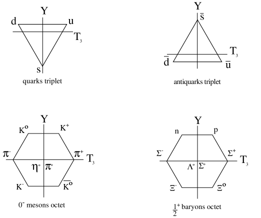
Figure 1.  : Examples of particle multiplets in the $SU(3)$ Quark Model

The description of hadrons in terms of quarks by means of the $SU(3)$ irreducible representations and their properties is called the $SU(3)$ Quark Model. One uses group theory methods, for instance the Young Tableaux technique, to decompose products of irreducible representations into sums. Thus the mesons ($B=0$) appear as composite states of a quark and an antiquark, and the baryons ($B=1$) as composite states of three quarks:

Mesons: $q\bar{q}=3\otimes\bar{3}=1\oplus 8$

Here the 1 are the $SU(3)$ meson singlets as the $\eta^{\prime}$ $\sim$ $(u\bar{u}+d\bar{d}+s\bar{s})$ with $J^{P}=0^{-}$, the $\Phi$ $\sim$ $(u\bar{u}+d\bar{d}+s\bar{s})$ with $J^{P}=1^{-}$… The 8 are the $SU(3)$ meson octets as the $0^{-}$ mesons, $\pi^{+}$ $\sim$ $u\bar{d}$, $K^{+}$ $\sim$ $u\bar{s}$ …; the $1^{-}$ mesons, $\rho^{+}$ $\sim$ $u\bar{d}$, $K^{*+}$ $\sim$ $u\bar{s}$…, and so on.

Baryons: $qqq=3\otimes 3\otimes 3=1\oplus 8\oplus 8\oplus 8\oplus 10$

Here the 1 are the $SU(3)$ baryon singlets; the 8 are the $SU(3)$ baryon octets as the $\frac{1}{2}^{+}$ baryons, $n$ $\sim$ $udd$, $p$ $\sim$ $uud$… ; the 10 are the $SU(3)$ decuplets as the $\frac{3}{2}^{+}$ baryons, $N^{*+}$ $\sim$ $uud$, $\Sigma^{*+}$ $\sim$ $suu$…, and so on.

Notice that the $SU(3)$ flavor symmetry is not an exact symmetry. As in the case of isospin symmetry, the mass differences within the members of a multiplet are signals of $SU(3)$ breaking. Similarly, the mass differences among the three quarks themselves are indications of this breaking as well. Although the breaking is certainly more sizeable in $SU(3)$ than in $SU(2)$, one can still deal with $SU(3)$ as an approximate symmetry.

Among the successful predictions of the Quark Model there are, for instance, the existence of some particles before their discovery as it is the case of the $\frac{3}{2}^{+}$ baryon $\Omega^{-}$ $\sim$ $sss$; and, in general, a large amount of the hadron properties are well described within this model. In particular, one may build up the hadron wave functions and compute some physical properties as, for instance, the hadron magnetic moments, in terms of the corresponding ones of the quarks components.

For example, the proton wave function with the spin up is:

$|p\uparrow>=\sqrt{\frac{1}{18}}|u\uparrow u\downarrow d\uparrow+u\downarrow u\uparrow d\uparrow-2u\uparrow u\uparrow d\downarrow+perm.>$

The predicted proton and neutron magnetic moments are:

$\mu_{p}=\frac{4}{3}\mu_{u}-\frac{1}{3}\mu_{d}$; $\mu_{n}=\frac{4}{3}\mu_{d}-\frac{1}{3}\mu_{u}$; with, $\mu_{q}=\frac{Q_{q}e}{2m_{q}}$

and their ratio is, therefore,

$\frac{\mu_{n}}{\mu_{p}}=-\frac{2}{3}$

which is rather close to its experimental measurement,

$\left.\frac{\mu_{n}}{\mu_{p}}\right|_{exp}=-0.68497945\pm 0.00000058$

The Quark Model has some noticeable failures which were the reason to abandon it as the proper model for strong interactions. The most famous one, from the historial point of view, is the so-called paradox of the $\Delta^{++}$. Its wave function for the case of spin up is given by,

$|\Delta^{++}\uparrow>\sim|u\uparrow u\uparrow u\uparrow>$

which is apparently totally symmetric since it is symmetric in space, flavor and spin. However, by Fermi-Dirac statistics it should be antisymmetric as it corresponds to an state with identical fermions. This apparent paradox, was solved by Gell-Mann with the proposal of the quarks carrying a new quantum number, the color and, in consequence, being non-identical from each other. Correspondingly, a quark $q$ can have three different colors, generically, $q_{i}\;i=1,2,3$. Since, this property of color is not seen in Nature, the colors of the quarks must be combined such that they produce colorless hadrons. In the group theory language it is got by requiring the hadrons to be in the singlet representations of the color group, $SU(3)_{C}$. Since the singlet representation is allways antisymmetric, by including this color wave function one gets finally the expected antisymmetry of the $\Delta^{++}$ total wave function.

5 QCD: The Gauge Theory of Strong Interactions

Quantum Chromodynamics is the gauge theory for strong interactions and has provided plenty of successful predictions so far [3].

It is based on the gauge symmetry of strong interactions, i.e. the local color transformations which leave its Hamiltonian (or Lagrangian) invariant. The gauge symmetry group that is generated by these color transformations is the non-abelian Lie group $SU(3)_{C}$. Here $C$ refers to colors and 3 refers to the three posible color states of the quarks which are assumed to be in the fundamental representation of the group having dimension three. The gluons are the gauge boson particles associated to this gauge symmetry and are eight of them as it corresponds to the number of $SU(3)$ generators. The gluons are the mediators of the strong interactions among quarks. Genericaly, the quarks and gluons are denoted by:

quarks: $q_{i}$, $i=1,2,3$;          gluons: $g_{\alpha}$, $\alpha=1,...,8$

The building of the QCD invariant Lagrangian is done by following the same steps as in the QED case. In particular, one applies the gauge principle as well with the particularities of the non-abelian group $SU(3)$ taken into account. Thus, the global symmetry $SU(3)$ of the Lagrangian for the strong interactions is promoted to local by replacing the derivative of the quark by its covariant derivative which in the QCD case is,

$D_{\mu}q\equiv\left(\partial_{\mu}-ig_{s}(\frac{\lambda_{\alpha}}{2})A_{\mu}^{\alpha}\right)q$

where,

$q=\left(\begin{array}[]{c}q_{1}\\ q_{2}\\ q_{3}\end{array}\right)$

$$\begin{array}[]{lcl}q_{i}&=&\;{\rm quark}\;{\rm fields};\;i=1,2,3\\ g_{s}&=&\;{\rm strong}\;{\rm coupling}\;{\rm constant}\\ \frac{\lambda_{\alpha}}{2}&=&SU(3)\;{\rm generators}\\ A_{\mu}^{\alpha}&=&\;{\rm gluon}\;{\rm fields};\;\alpha=1,...,8\end{array}$$

The QCD Lagrangian is then written in terms of the quarks and their covariant derivatives and contains in addition the kinetic term for the gluon fields,

$\displaystyle{\cal L}_{QCD}=\sum_{q}\overline{q}(x)(iD{/}-m_{q})q(x)-\frac{1}{4}F_{\mu\nu}^{\alpha}(x)F^{\mu\nu}_{\alpha}(x)$

The gluon field strength is,

$F_{\mu\nu}^{\alpha}(x)=\partial_{\mu}A_{\nu}^{\alpha}(x)-\partial_{\nu}A_{\mu}^{\alpha}(x)+g_{s}f^{\alpha\beta\gamma}A_{\mu\beta}A_{\nu\gamma}$

and contains a bilinear term in the gluon fields as it corresponds to a non-abelian gauge theory with structure constants $f^{\alpha\beta\gamma}$ ($\alpha,\beta,\gamma=1,...,8$).

It can be shown that the above Lagrangian is invariant under the following $SU(3)$ gauge transformations,

$\left\{\begin{array}[]{lcl}q(x)&\rightarrow&e^{i\theta_{\alpha}(x)\frac{\lambda^{\alpha}}{2}}q(x)\\ D_{\mu}q(x)&\rightarrow&e^{i\theta_{\alpha}(x)\frac{\lambda^{\alpha}}{2}}D_{\mu}q(x)\\ A_{\mu}^{\alpha}(x)&\rightarrow&A_{\mu}^{\alpha}(x)-\frac{1}{g_{s}}\partial_{\mu}\theta^{\alpha}(x)+f^{\alpha\beta\gamma}\theta_{\beta}(x)A_{\mu\gamma}(x)\end{array}\right.$

where $\theta_{\alpha}(x)\;\alpha=1,...,8$ are the parameters of the transformation.

Similarly to the QED case, the gauge interactions among the quarks and gluons are contained in the $\bar{q}iD{/}q$ term,

$\bar{q}g_{s}\frac{\lambda^{\alpha}}{2}A_{\mu}^{\alpha}\gamma^{\mu}q$

There is, however, an important difference with the QED case. The gluon kinetic term $F_{\mu\nu}^{\alpha}F^{\mu\nu}_{\alpha}$ contains a three gluons term and a four gluons term. These are precisely the selfinteraction gluon vertices which are genuine of a non-abelian theory.

5.1 $SU(3)$ Group properties

In this section we list the basic properties of the $SU(3)$ group which are relevant for QCD and in particular for the computation of color factors in processes mediated by strong interactions.

$SU(3)$ is the set of $3\times 3$ unitary matrices with unit determinant. Any element of $SU(3)$, $U$, can be written in terms of its 8 generators, $\frac{\lambda_{\alpha}}{2}$ and a set of 8 real parameters $\theta_{\alpha}$ as,

$U=e^{i\theta^{\alpha}\frac{\lambda_{\alpha}}{2}}$; $\alpha=1,...,8$

The generators are $3\times 3$ traceless hermitian matrices $\frac{\lambda_{\alpha}}{2}$ and are given in terms of the so-called Gell-Mann matrices, $\lambda_{\alpha}$,

$$\lambda_{1}=\left(\begin{array}[]{ccc}0&1&0\\ 1&0&0\\ 0&0&0\end{array}\right)\;\;,\;\;\lambda_{2}=\left(\begin{array}[]{ccc}0&-i&0\\ i&0&0\\ 0&0&0\end{array}\right)\;\;,\;\;\lambda_{3}=\left(\begin{array}[]{ccc}1&0&0\\ 0&-1&0\\ 0&0&0\end{array}\right)$$

$$\lambda_{4}=\left(\begin{array}[]{ccc}0&0&1\\ 0&0&0\\ 1&0&0\end{array}\right)\;\;,\;\;\lambda_{5}=\left(\begin{array}[]{ccc}0&0&-i\\ 0&0&0\\ i&0&0\end{array}\right)$$

$$\lambda_{6}=\left(\begin{array}[]{ccc}0&0&0\\ 0&0&1\\ 0&1&0\end{array}\right)\;\;,\;\;\lambda_{7}=\left(\begin{array}[]{ccc}0&0&0\\ 0&0&-i\\ 0&i&0\end{array}\right)\;\;,\;\;\lambda_{8}=\frac{1}{\sqrt{3}}\left(\begin{array}[]{ccc}1&0&0\\ 0&1&0\\ 0&0&-2\end{array}\right)$$

Some basic properties of the $SU(3)$ generators are:

$\displaystyle\left[\frac{\lambda_{\alpha}}{2},\frac{\lambda_{\beta}}{2}\right]\;=\;if_{\alpha\beta\gamma}\frac{\lambda_{\gamma}}{2}$           $\displaystyle Tr\left(\frac{\lambda_{\alpha}}{2}\frac{\lambda_{\beta}}{2}\right)\;=\;\frac{1}{2}\delta_{\alpha\beta}$

The tensor $f_{\alpha\beta\gamma}$ is totally antisymmetric and its elements are the structure constants of $SU(3)$. The non-vanishing elements are,

$f_{123}=1$, $f_{147}=\frac{1}{2}$, $f_{156}=-\frac{1}{2}$, $f_{246}=\frac{1}{2}$, $f_{257}=\frac{1}{2}$,

$f_{345}=\frac{1}{2}$, $f_{367}=-\frac{1}{2}$, $f_{458}=\sqrt{\frac{3}{2}}$ $f_{678}=\sqrt{\frac{3}{2}}$

Some useful relations for practical computations and relevant group factors are,

$$\delta_{\alpha\beta}C_{A}\;=\;\sum_{\gamma\delta}f_{\alpha\gamma\delta}f_{\beta\gamma\delta}\;\;;\;\;C_{A}=3$$

$$\delta_{ik}C_{F}\;=\;\sum_{\alpha l}\frac{\lambda^{\alpha}_{il}}{2}\frac{\lambda^{\alpha}_{lk}}{2}\;\;;\;\;C_{F}=\frac{4}{3}$$

$$\delta_{\alpha\beta}T_{F}\;=\;\sum_{ki}\frac{\lambda^{\alpha}_{ik}}{2}\frac{\lambda^{\beta}_{ki}}{2}\;\;;\;\;T_{F}=\frac{1}{2}$$

$$(i,k=1,2,3\;;\;\alpha,\beta,\gamma,\delta=1,...,8)$$

5.2 Computing color factors in QCD

For practical computations, sometimes it is convenient to define color factors associated to a physical proccess in QCD. These color factors are genuine of QCD and can be computed apart by using the $SU(3)$ group relations.

For illustrative purposes, we present here one particular example: the computation of the color factor associated to the scattering proccess of two different quarks, $qq^{\prime}\rightarrow qq^{\prime}$.

There is just one Feynman diagram contributing to the scattering amplitude of this proccess which is the diagram with one gluon exchanged in the t-channel. Notice that this diagram is similar to the one contributing to the QED proccess $e^{-}\mu^{-}\rightarrow e^{-}\mu^{-}$ where one photon is exchanged in the t-channel.

One can use the known result from QED for the spin-averaged squared amplitude of the proccess $e^{-}\mu^{-}\rightarrow e^{-}\mu^{-}$ in terms of the Mandelstam variables, $s$, $t$, and $u$,

$$\overline{|F|}^{2}=2e^{4}\left(\frac{s^{2}+u^{2}}{t^{2}}\right)$$

and by simply replacing the electromagnetic coupling constant $e$ by the strong coupling constant $g_{s}$ and by adding a color factor $F_{C}$ one obtains the corresponding squared amplitude of the proccess $qq^{\prime}\rightarrow qq^{\prime}$, at tree level in QCD,

$$\overline{|F|}^{2}=F_{C}2g_{s}^{4}\left(\frac{s^{2}+u^{2}}{t^{2}}\right)$$

The color factor $F_{C}$ can be now computed apart. From the QCD Feynman rules for the quark-gluon-quark vertex and for the gluon propagator; and by averaging in initial colors and summing in final colors one gets,

$$F_{C}=\frac{1}{9}\sum_{ijlm\\ \alpha\beta\alpha^{\prime}\beta^{\prime}}\left(\frac{\lambda_{ij}^{\alpha}}{2}\right)\delta_{\alpha\beta}\left(\frac{\lambda_{lm}^{\beta}}{2}\right)\left(\frac{\lambda_{ij}^{\alpha^{\prime}}}{2}\right)^{*}\delta_{\alpha^{\prime}\beta^{\prime}}\left(\frac{\lambda_{lm}^{\beta^{\prime}}}{2}\right)^{*}$$

The above expression can be simplified by using the properties of the $SU(3)$ generators,

$$\begin{array}[]{lcl}F_{C}&=&\frac{1}{9}\sum_{\alpha\alpha^{\prime}}\left[\sum_{ij}\left(\frac{\lambda_{ij}^{\alpha}}{2}\right)\left(\frac{\lambda_{ji}^{\alpha^{\prime}}}{2}\right)\right]\left[\sum_{lm}\left(\frac{\lambda_{lm}^{\alpha}}{2}\right)\left(\frac{\lambda_{ml}^{\alpha^{\prime}}}{2}\right)\right]\\ &&\\ &=&\frac{1}{9}\sum_{\alpha\alpha^{\prime}}\left[\delta_{\alpha\alpha^{\prime}}T_{F}\right]\left[\delta_{\alpha\alpha^{\prime}}T_{F}\right]\\ &&\\ &=&\frac{2}{9}\end{array}$$

6 Weak Interactions before The Electroweak Theory

The existence of new interactions of weak strength were proposed to explain the experimental data indicating long lifetimes in the decays of known particles, as for instance,

$$n\rightarrow pe^{-}\overline{\nu}_{e}\;;\;\tau_{n}=920\;sec$$

$$\pi^{-}\rightarrow\mu^{-}\overline{\nu}_{\mu}\;;\;\tau_{\pi^{-}}=2.6\times 10^{-8}\;sec$$

$$\mu^{-}\rightarrow e^{-}\overline{\nu}_{e}\nu_{\mu}\;;\;\tau_{\mu}=2.2\times 10^{-6}\;sec$$

These are much longer lifetimes than the typical decays mediated by strong interactions as,

$$\Delta\rightarrow p\pi\;;\;\tau_{\Delta}=10^{-23}\;sec$$

and by electromagnetic interactions as,

$$\pi^{0}\rightarrow\gamma\gamma\;;\;\tau_{\pi^{0}}=10^{-16}\;sec$$

The history of weak interactions before the formulation of the Standard $SU(2)_{L}\times U(1)_{Y}$ Theory is an interesting example of the relevant interplay between theory and experiment. There were a sequence of proposed models which were confronted systematically with the abundant experimental data and which needed to be either refined or rejected in order to be compatible with the observations. All this relevant phenomenology of weak interactions together with the advent of the gauge theories in particle physics led finally to the formulation of the Electroweak Theory, i.e. the gauge theory of electroweak interactions. Among the most relevant predecessor theories of electroweak interactions are the following: Fermi Theory, V-A Theory of Feynman and Gell-Mann and the IVB theory of Lee, Yang and Glashow.

6.1 Fermi Theory of Weak Interactions

In 1934 Fermi proposed the four-fermion interactions theory [10] in order to describe the neutron $\beta$-decay $n\rightarrow pe^{-}\overline{\nu}_{e}$,

${\cal L}_{F}=-\frac{G_{F}}{\sqrt{2}}\left[\overline{p}(x)\gamma_{\lambda}n(x)\right]\left[\overline{e}(x)\gamma^{\lambda}\nu_{e}(x)\right]+h.c.$

where the fermion field operators are denoted by their particle names and,

$$G_{F}=1.167\times 10^{-5}\;GeV^{-2}$$

is the so-called Fermi constant which provides the effective dimensionful coupling of the weak interactions.

The Fermi Lagrangian above assumes a vector structure, as in the electromagnetic case, for both the hadronic current, $J_{\lambda}^{(h)}(x)=\overline{p}(x)\gamma_{\lambda}n(x)$, and the leptonic current, $J_{\lambda}^{(l)}(x)=\overline{\nu}_{e}(x)\gamma_{\lambda}e(x)$; and postulates a local character for the four fermion interactions, namely, the two currents are contracted at the same space-time point $x$.

Due precisely to the above vector structure of the weak currents, the Fermi Lagrangian does not explain the observed parity violation in weak interactions.

6.2 Parity Violation and the V-A form of charged weak interactions

The observation of Kaon decays in two different final states with opposite parities,

$$K^{+}\rightarrow\pi^{+}\pi^{0}\;\;{\rm and}\;\;K^{+}\rightarrow\pi^{+}\pi^{+}\pi^{-}$$

led Lee and Yang in 1956 to suggest the non-conservation of parity in the weak interactions responsible for these decays [11]. Parity violation was discovered by Wu and collaborators in 1957 [12] by analizing the decays of $Co$ nuclei

$${}^{60}Co\rightarrow^{60}Ni^{*}\;e^{-}\;\overline{\nu}_{e}$$

which proceed via neutron decay $n\rightarrow pe^{-}\overline{\nu}_{e}$.

The nuclei are polarized by the action of an external magnetic field such that the angular momenta for $Co$ and $Ni$ are $J=5$ and $J=4$ respectively, both aligned in the direction of the external field. By conservation of the total angular momentum, the angular momentum of the combined system electron-antineutrino is inferred to be $J(e^{-}\;\overline{\nu}_{e})=1$ and must be aligned with the other angular momenta. Therefore both the electron and the antineutrino must have their spins polarized in this same direction. The electron from the decay is seeing always moving in the opposite direction to the external field. By total momentum conservation, the undetected antineutrino is, in consequence, assumed to be moving in the opposite direction to the electron. Altogether leads to the conclusion that the produced electron has negative helicity and the antineutrino has positive helicity. Therefore, the charged weak currents responsible for these decays always produce left-handed electrons and right-handed antineutrinos. The non-observation of left-handed antineutrinos nor right-handed neutrinos in processes mediated by charged weak interactions is a signal of parity violation since the parity transformation changes a left-handed fermion into the corresponding right-handed fermion and viceversa. In fact, it is an indication of maximal parity violation which implies that the charged weak current must be neccessarily of the vector minus axial vector form,

$J_{\mu}\sim V_{\mu}-A_{\mu}$

Let us see this in more detail. The vector and axial vector currents transform under parity as follows,

$$V^{\mu}=\overline{\Psi}\gamma^{\mu}\Psi\stackrel{{\scriptstyle P}}{{\longrightarrow}}\left\{\begin{array}[]{l}+\overline{\Psi}\gamma^{0}\Psi\\ -\overline{\Psi}\gamma^{k}\Psi\;;\;k=1,2,3\end{array}\right.$$

$$A^{\mu}=\overline{\Psi}\gamma^{\mu}\gamma^{5}\Psi\stackrel{{\scriptstyle P}}{{\longrightarrow}}\left\{\begin{array}[]{l}-\overline{\Psi}\gamma^{0}\gamma^{5}\Psi\\ +\overline{\Psi}\gamma^{k}\gamma^{5}\Psi\;;\;k=1,2,3\end{array}\right.$$

Therefore the various products transform as,

$$V_{\mu}V^{\mu}\stackrel{{\scriptstyle P}}{{\longrightarrow}}V_{\mu}V^{\mu}$$

$$A_{\mu}A^{\mu}\stackrel{{\scriptstyle P}}{{\longrightarrow}}A_{\mu}A^{\mu}$$

$$A_{\mu}V^{\mu}\stackrel{{\scriptstyle P}}{{\longrightarrow}}-A_{\mu}V^{\mu}$$

Any combination of vector and axial vector currents as $J_{\mu}\sim\alpha V_{\mu}+\beta A_{\mu}$ will generate parity violation in the Lagrangian, ${\cal L}\sim J_{\mu}J^{\mu+}$. But maximal parity violation is only reached if $J_{\mu}\sim V_{\mu}-A_{\mu}$, since

$$J_{\mu}J^{\mu+}\sim(V_{\mu}-A_{\mu})(V^{\mu}-A^{\mu})\stackrel{{\scriptstyle P}}{{\longrightarrow}}(V_{\mu}+A_{\mu})(V^{\mu}+A^{\mu})$$

which translates into that charged weak interactions only couple to left-handed fermions or right-handed antifermions. This can be seen simply by rewritting the current $J_{\mu}$ in terms of the field components. For instance, the leptonic current can be rewritten in terms of the left-handed fields as,

$$J_{\mu}\sim V_{\mu}-A_{\mu}=\overline{\nu}_{e}\gamma_{\mu}(1-\gamma_{5})e=2\overline{(\nu_{e})_{L}}\gamma_{\mu}e_{L}$$

6.3 V-A Theory of Charged Weak Interactions

After the discovery of parity violation in weak interactions, Feynman and Gell-Mann in 1958 proposed the V-A Theory [13] which incorporated the success of the Fermi Theory and solved the question of parity non-conservation by postulating instead a V-A form for the charged weak current. The current-current interactions are, like in the Fermi Theory, of local character, being contracted at the same space-time point. The effective weak copling is, as in the Fermi Theory, given by the Fermi constant, $G_{F}$.

The Lagrangian of the V-A Theory for the two first fermion generations is as follows,

${\cal L}_{V-A}=-\frac{G_{F}}{\sqrt{2}}J_{\mu}^{CC}(x)J^{\mu CC+}(x)$

$J_{\mu}^{CC}=\overline{\nu}_{e}\gamma_{\mu}(1-\gamma_{5})e+\overline{\nu}_{\mu}\gamma_{\mu}(1-\gamma_{5})\mu+\overline{u}\gamma_{\mu}(1-\gamma_{5})d^{\prime}$

Notice that the $d$-quark field appearing in this Lagrangian, denoted by $d^{\prime}$, is the weak interactions $d$-quark eigenstate which is different than the $d$-quark mass eigenstate, denoted in these lectures by $d$. They are related by a rotation of the so-called Cabibbo angle $\theta_{c}$,

$$d^{\prime}=cos\theta_{c}d+sin\theta_{c}s$$

The idea of the rotated d-quark states was proposed by Cabibbo in 1963 [14] to account for weak decays of ’strange’ particles and, in particular, to explain the suppression factor of the kaon decay rate as compared to the pion decay rate which experimentally was found to be about $\frac{1}{20}$. By comparing the theoretical prediction from the V-A Theory with the experimental data, the numerical value of the $\theta_{c}$ angle is inferred,

$\frac{\Gamma(K^{-}\rightarrow\mu^{-}\overline{\nu}_{\mu})}{\Gamma(\pi^{-}\rightarrow\mu^{-}\overline{\nu}_{\mu})}\sim\frac{sin^{2}\theta_{c}}{cos^{2}\theta_{c}}\sim\frac{1}{20}$      $\Longrightarrow$      $\theta_{c}\simeq 13^{\circ}$

The value of the effective coupling of the weak interactions, $G_{F}$ is deduced from the meassurement of the $\mu$ lifetime,

$$\tau_{\mu}^{\rm exp}=2.2\times 10^{-6}\;sec$$

The prediction in the V-A Theory to tree level and by neglecting the electron mass is,

$$\frac{1}{\tau_{\mu}}=\Gamma(\mu^{-}\rightarrow e^{-}\overline{\nu}_{e}\nu_{\mu})=\frac{G_{F}^{2}m_{\mu}^{5}}{192\pi^{3}}$$

and from this,

$G_{F}=1.167\times 10^{-5}\;GeV^{-2}$

The V-A Theory described reasonably well the phenomenology of weak interactions until the discovery of the neutral currents in 1973 [15]. Notice that the neutral currents were not included in the formulation of the V-A Theory. Besides, The V-A Theory presented some non-appealing properties from the point of view of the consistency of the theory itself. In particular, the V-A Theory violates unitarity and it is a non-renormalizable theory. The unitarity violation property can be seen, for instance, by comparing the prediction in the V-A Theory of the cross section for elastic scattering of electron and neutrino,

$$\sigma_{V-A}(\nu e^{-}\rightarrow\nu e^{-})=\frac{G_{F}^{2}}{6\pi}s$$

with the unitarity bound for the total cross section which is obtained from the general requirement of unitarity of the scattering S-matrix,

$$SS^{+}=S^{+}S=I\hskip 5.69046pt\Longrightarrow\hskip 5.69046pt|a_{J}(s)|^{2}\leq 1\;\forall J\hskip 5.69046pt\Longrightarrow$$

$$\sigma(s)_{\rm tot}=\frac{16\pi}{s}\sum_{J}(2J+1)|a_{J}(s)|^{2}\leq\frac{16\pi}{s}\sum_{J}(2J+1)$$

It is clear that for high energies the prediction from the V-A Theory surpasses the unitarity bound and, therefore, it should not be trusted. It happens roughly at $\sqrt{s}\sim 300\;GeV$.

The non-renormalizability of the V-A Theory can be seen, for instance, by computing loop contributions to the cross section and realizing that there appear quadratic divergences which cannot be absorved into redefinitions of the parameters of this theory. As in the previous discussion on unitarity, it is due to the ’bad’ behaviour of the V-A Theory at high energies. The V-A Theory is said to be non-predictive at high energies and it should only be used as an effective theory at low enough energies.

6.4 Intermediate Vector Boson Theory

The Intermediate Vector Boson (IVB) Theory of weak interactions assumed that these are mediated by the exchange of massive vector bosons with spin, $s=1$. First, it was proposed the existence of intermediate charged vector bosons $W^{\pm}$ for the charged weak interactions [16] and later the intermediate neutral vector boson $Z$ for the neutral weak interactions [17]. Notice that these bosons were not true gauge bosons yet.

The interaction Lagrangian of the IVB Theory, including both the charged (CC) and the neutral (NC) currents, is given by,

${\cal L}_{IVB}={\cal L}_{CC}+{\cal L}_{NC}$ ${\cal L}_{CC}=\frac{g}{\sqrt{2}}(J_{\mu}W^{\mu+}+J_{\mu}^{+}W^{-\mu})$ ${\cal L}_{NC}=\frac{g}{cos\theta_{w}}J_{\mu}^{NC}Z^{\mu}$

where,

$J_{\mu}=\sum_{l}\overline{\nu}_{l}\gamma_{\mu}\left(\frac{1-\gamma_{5}}{2}\right)l+\sum_{q}\overline{q}\gamma_{\mu}\left(\frac{1-\gamma_{5}}{2}\right)q^{\prime}$ $J_{\mu}^{NC}=\sum_{f=l,q}g_{L}^{f}\overline{f}\gamma_{\mu}\left(\frac{1-\gamma_{5}}{2}\right)f+\sum_{f\neq\nu}g_{R}^{f}\overline{f}\gamma_{\mu}\left(\frac{1+\gamma_{5}}{2}\right)f$

Here the $W^{\pm}_{\mu}$ and $Z_{\mu}$ are the charged and neutral intermediate vector bosons respectively and $g$ is the dimensionless weak coupling. The weak angle, $\theta_{w}$, defines the rotation in the neutral sector from the weak eigenstates to the physical mass eigenstates, and relates the weak coupling to the electromagnetic coupling, $g=\frac{e}{sin\theta_{w}}$.

Notice that the current-current interactions are non-local, in contrast to the V-A Theory, due to the propagation of the intermediate bosons. Besides, the new proposed neutral currents have both V-A and V+A components, although experimentaly it is known that the V-A component dominates.

The prediction of neutral currents in 1961 [17] was corroborated experimentally 12 years later! in neutrino-hadron scattering by the Gargamelle collaboration at CERN [15]. It was a great success of the IVB Theory which was incorporated later into the construction of the SM.

The relation between the parameters of the IVB Theory and the V-A Theory, which is also incorporated in the construction of the SM, can be obtained by comparison of the predictions from the two theories for $e\nu\rightarrow e\nu$ scattering at low energies ($\sqrt{s}<<M_{W}$),

$\frac{G_{F}}{\sqrt{2}}=\frac{g^{2}}{8M_{W}^{2}}$

Finally, the IVB Theory is not free of problems either. It shares with the V-A Theory the problems of non-renormalizability and violation of unitarity at high energies. At low energies, say below the $M_{W}$ threshold, the IVB Theory is a well behaved effective theory of the weak interactions, but above it the theory behaves badly. The problem of non-renormalizability can be seen for instance by studing the $e^{+}e^{-}\rightarrow e^{+}e^{-}$ scattering proccess at one loop. There are one-loop diagramms with $W$ bosons propagating in the internal lines that diverge quadratically at high energies due to the bad behaviour of the $W$ boson propagator in the IVB Theory,

$$\left(-i\Delta_{W}\right)_{IVB}\stackrel{{\scriptstyle k^{2}>>M_{W}^{2}}}{{\longrightarrow}}\frac{1}{M_{W}^{2}}$$

This should be compared with the well behaved $W$ boson propagator in the Electroweak Gauge Theory,

$$\left(-i\Delta_{W}\right)_{\rm gauge}\stackrel{{\scriptstyle k^{2}>>M_{W}^{2}}}{{\longrightarrow}}\frac{1}{k^{2}}$$

The violation of the unitarity bound occurs at slightly higher energies that in the V-A Theory case. For instance, the cross-section for the production of two longitudinal gauge bosons from neutrinos in the IVB Theory at tree level is,

$$\sigma_{IVB}(\nu\overline{\nu}\rightarrow W_{L}^{+}W_{L}^{-})\sim\frac{g^{4}}{M_{W}^{4}}s$$

which surpasses the unitarity bound at approximately, $\sqrt{s}\sim 500\;GeV$. Notice that there is just one contributing diagramm, the one with an electron in the t-channel. Notice also that the IVB Theory does not include the vector bosons self-interactions which are generic of non-abelian gauge theories. These are precisely the ’repairing’ interactions ocurring in the Electroweak Theory . The prediction from the SM for the previous scattering proccess includes the contribution from an extra diagramm with a $Z$ boson exchanged in the s-channel which couples to the final $W_{L}^{+}W_{L}^{-}$ pair with a typical non-abelian Yang Mills coupling. This new diagramm cancels the bad high energy behaviour of the previous one. This dramatic cancellation also occurs in many other proccesses. See, for instance, the meassurement of the cross-section for $e^{+}e^{-}\rightarrow W^{+}W^{-}$ at LEP presented in Nodulman’s lectures, where these cancellations are shown.

7 Building The Electroweak Theory

7.1 Some notes on History

The proposal of the symmetry group for the Electroweak Theory, $SU(2)_{L}\times U(1)_{Y}$, was done by Glashow in 1961 [17]. His motivation was rather to unify weak and electromagnetic interactions into a symmetry group that contained $U(1)_{em}$. The predictions included the existence of four physical vector boson eigenstates, $W^{\pm}$, $Z$, and $\gamma$, obtained from rotations of the weak eigenstates. In particular, the rotation by the weak angle $\theta_{w}$ which defines the $Z$ weak boson was introduced already in this work. The massive weak bosons $W^{\pm}$ and $Z$ were considered as the exchanged bosons in the weak interactions, but they were not considered yet as gauge bosons. The vector boson masses $M_{W}$ and $M_{Z}$ were parameters introduced by hand and the interaction Lagrangian was that of the IVB Theory.

Another key ingredient for the building of the Electroweak Theory is provided by the Goldstone Theorem which was initiated by Nambu in 1960 and proved and studied with generality by Goldstone in 1961 and by Goldstone, Salam and Weinberg in 1962 [18]. This theorem states the existence of massless spinless particles as an implication of spontaneous symmetry breaking of global symmetries.

The spontaneous symmetry breaking of local (gauge) symmetries, needed for the breaking of the electroweak symmetry $SU(2)_{L}\times U(1)_{Y}$, was studied by P. Higgs, F.Englert and R.Brout, Guralnik, Hagen and Kibble in 1964 and later [19]. These works were inspired in previous studies within the context of condensed-matter physics as those by Nambu and Jona-Lasinio on BCS Theory of superconductivity and works by Schwinger in 1962 and by Anderson in 1963 [20]. The procedure for this spontaneous breakdown of gauge symmetries is referred to as the Higgs Mechanism.

The Electroweak Theory as it is known nowadays was formulated by Weinberg in 1967 and by Salam in 1968 who incorporated the idea of unification of Glashow [1]. This Theory, commonly called Glashow-Weinberg-Salam Model or SM, was built with the help of the gauge principle and the knowledgde of gauge theories and incorporated all the good phenomelogical properties of the pregauge theories of the weak interactions, and in particular those of the IVB theory. The SM is indeed a gauge theory based on the gauge symmetry of the electroweak interactions $SU(2)_{L}\times U(1)_{Y}$ and the intermediate vector bosons, $\gamma$, $W^{\pm}$ and $Z$ are the four associated gauge bosons. The gauge boson masses, $M_{W}$ and $M_{Z}$, are generated by the Higgs Mechanism in the Electroweak Theory and, as a consequence, it respects unitarity at all energies and is renormalizable.

The important proof of renormalizability of gauge theories with and without spontaneous symmetry breaking was provided by ’t Hooft in 1971 [21].

The first firm indication that the Sandard Model was the correct theory of electroweak interactions was probably the discovery of Neutral Currents in 1973 [15] which included the first meassurement of $sin^{2}\theta_{w}$. By using this experimental input for $\theta_{w}$ and the values of the electromagnetic coupling and $G_{F}$, the SM provided the first estimates for $M_{W}$ and $M_{Z}$ at that time which were already very close to the present values.

Another important ingredients of the SM are: fermion family replication, quark mixing and CP violation. After the proposal of the $d-s$ quark mixing given by the Cabibbo angle [14], the charm quark was postulated [22] as the companion of the $s$ quark in the charged weak interactions. Futhermore, Glashow, Iliopoulos and Maiani showed in 1970 [23] that any sensible weak interaction theory must have this extra associated hadronic current in order to suppress to an acceptable level the induced strangeness-changing-neutral current effects. This suppression mechanism of flavour-changing-neutral currents (FCNC), usualy called GIM Mechanism, although invented before the general acceptance of gauge theories, can best be explained in that context. The existence of the $c$ quark was confirmed in 1974 [24] with the discovery of the $J-\Psi$ particle which is interpreted as a $c\overline{c}$ bound state. With the discovery of the $\tau$ and $\nu_{\tau}$ leptons [25] and the $b$ quark [26], the fermion scenario with three families was set in. Finally, the discovery of the top quark in 1994 (17 years later!) [27] has completed this scenario. The quark mixing in the three generations case is given by the so-called Cabibbo-Kobayashi-Maskawa matrix [28] which incorporates the needed phase for CP violation in the SM.

The gold success of the SM was clearly the discovery of the gauge bosons $W^{\pm}$ and $Z$ at the SpS collider at CERN in 1983 [30]. Since then there have been plenty of succesfull tests of the SM.

7.2 Choice of the group $SU(2)_{L}\times U(1)_{Y}$

In order to follow the argument for the choice of the relevant group in the Electroweak Theory, $SU(2)_{L}\times U(1)_{Y}$, it is sufficient to consider the $e^{-}\nu_{e}$ component of the charged weak current that we write now in the form,

$$J_{\mu}=\overline{\nu}\gamma_{\mu}\left(\frac{1-\gamma_{5}}{2}\right)e=\overline{\nu_{L}}\gamma_{\mu}e_{L}=\overline{l_{L}}\gamma_{\mu}\sigma_{+}l_{L}$$

$$J_{\mu}^{+}=\overline{e}\gamma_{\mu}\left(\frac{1-\gamma_{5}}{2}\right)\nu=\overline{e_{L}}\gamma_{\mu}\nu_{L}=\overline{l_{L}}\gamma_{\mu}\sigma_{-}l_{L}$$

and we have introduced the lepton doublet notation and the $\sigma_{i}\;(i=1,2,3)$ Pauli matrices,

$$l_{L}=\left(\begin{array}[]{c}\nu_{L}\\ e_{L}\end{array}\right)\;,\;\overline{l_{L}}=\left(\begin{array}[]{cc}\overline{\nu_{L}}&\overline{e_{L}}\end{array}\right)\;,\;\sigma_{\pm}=\frac{1}{2}(\sigma_{1}\pm i\sigma_{2})$$

$$\sigma_{1}=\left(\begin{array}[]{cc}0&1\\ 1&0\end{array}\right)\;,\;\sigma_{2}=\left(\begin{array}[]{cc}0&-i\\ i&0\end{array}\right)\;,\;\sigma_{3}=\left(\begin{array}[]{cc}1&0\\ 0&-1\end{array}\right)$$

The $2\times 2$ matrices $T_{i}=\frac{\sigma_{i}}{2}\;i=1,2,3$ are the three generators of $SU(2)$.

Notice that in the charged currents there are just two generators $T_{1}$ and $T_{2}$. A third generator $T_{3}$ is needed in order to close the $SU(2)$ algebra. This implies the formulation of the third current that is relevant for electroweak interactions,

$$J_{\mu}^{3}=\overline{l_{L}}\gamma_{\mu}\frac{\sigma_{3}}{2}l_{L}=\frac{1}{2}(\overline{\nu_{L}}\gamma_{\mu}\nu_{L}-\overline{e_{L}}\gamma_{\mu}e_{L})$$

The weak isospin group is the $SU(2)$ group that is generated by these three generators and is usually denoted by $SU(2)_{L}$, where the subscript $L$ refers to the left-handed character of the three weak currents. The weak isospin algebra is correspondingly,

$$\left[\frac{\sigma_{i}}{2},\frac{\sigma_{j}}{2}\right]=i\epsilon_{ijk}\frac{\sigma_{k}}{2}$$

where the $SU(2)$ structure constants are the completely antisymmetric Levi-Civita symbols $\epsilon_{ijk}$.

By Noether’s Theorem there are three associated conserved weak charges,

$$T^{i}=\int d^{3}xJ_{0}^{i}(x)\;,\;i=1,2,3$$

It is interesting to notice that the above introduced neutral weak current is none of the two physical known neutral currents, $J_{\mu}^{em}$ and $J_{\mu}^{NC}$. Futhermore, none of these two currents have definite properties under $SU(2)_{L}$ transformations, whereas $J_{\mu}^{3}$ does. With the motivation of unifying the electromagnetic and weak interactions, Glashow proposed to include the electromagnetic current by adding to $SU(2)_{L}$ a new $U(1)$ group which should be different than $U(1)_{em}$ in order to the get the proper conmutation relations among the $U(1)$ and $SU(2)_{L}$ generators. The new proposed group is the weak hypercharge group $U(1)_{Y}$ with one generator $\frac{Y}{2}$ which indeed, as it must be, conmutes with the three $SU(2)_{L}$ generators. The associated neutral current is the weak hypercharge current, $J_{\mu}^{Y}$, and the conserved charge is the weak hypercharge $Y$. Within this formalism there is some sort of electromagnetic and weak interactions unification since the $U(1)_{em}$ group appears as a subgroup of the total electroweak group,

$$U(1)_{em}\subset SU(2)_{L}\times U(1)_{Y}$$

The relation among the charges associated to the three neutral currents, $J_{\mu}^{em}$, $J_{\mu}^{3}$ and $J_{\mu}^{Y}$, is a replica of the Gell-Mann Nishijima relation,

$Q=T_{3}+\frac{Y}{2}$

where now,

$$Q={\rm electric\;charge}\;,\;T_{3}={\rm weak\;isospin}\;,\;Y={\rm weak\;hypercharge};$$

and the corresponding relation among the currents is,

$$J_{\mu}^{em}=J_{\mu}^{3}+J_{\mu}^{Y}$$

Therefore, if the following are used as inputs

$$J_{\mu}^{em}=(-1)\overline{e_{L}}\gamma_{\mu}e_{L}+(-1)\overline{e_{R}}\gamma_{\mu}e_{R}$$

$$J_{\mu}^{3}=\left(-\frac{1}{2}\right)\overline{e_{L}}\gamma_{\mu}e_{L}+\left(\frac{1}{2}\right)\overline{\nu_{L}}\gamma_{\mu}\nu_{L}$$

one can get $J_{\mu}^{Y}$ and the orthogonal combination $J_{\mu}^{NC}$ as outputs,

$$J_{\mu}^{Y}=2(J_{\mu}^{em}-J_{\mu}^{3})=(-1)\overline{e_{L}}\gamma_{\mu}e_{L}+(-2)\overline{e_{R}}\gamma_{\mu}e_{R}+(-1)\overline{\nu_{L}}\gamma_{\mu}\nu_{L}$$

$$J_{\mu}^{NC}\perp J_{\mu}^{em}\Rightarrow$$

$$J_{\mu}^{NC}=c_{w}^{2}J_{\mu}^{3}-s_{w}^{2}\frac{J_{\mu}^{Y}}{2}=(-\frac{1}{2}+s_{w}^{2})\overline{e_{L}}\gamma_{\mu}e_{L}+(s_{w}^{2})\overline{e_{R}}\gamma_{\mu}e_{R}+(\frac{1}{2})\overline{\nu_{L}}\gamma_{\mu}\nu_{L}$$

where,

$$c_{w}=cos\theta_{w}\;;\;s_{w}=sin\theta_{w}\;;\;\theta_{w}={\rm weak\;angle}$$

Notice that the currents that couple to the physical neutral bosons $A_{\mu}$ and $Z_{\mu}$ are $J_{\mu}^{em}$ and $J_{\mu}^{NC}$ respectively, and it is this last one, $J_{\mu}^{NC}$, that inherits the generic name of neutral current.

From the above expressions for the neutral currents, one can also extract the values of the corresponding charges and couplings. For instance, from $J_{\mu}^{NC}$ one gets the relevant factors in the weak neutral couplings to electrons and neutrinos , $g_{L}^{e}=-\frac{1}{2}+s_{w}^{2}$, $g_{R}^{e}=s_{w}^{2}$, $g_{L}^{\nu}=\frac{1}{2}$ and $g_{R}^{\nu}=0$.

If one includes the contributions from all the quarks and leptons of the three families, the neutral currents are written generically as:

$$J_{\mu}^{Y}=\sum_{f}Y_{f_{L}}\overline{f_{L}}\gamma_{\mu}f_{L}+\sum_{f}Y_{f_{R}}\overline{f_{R}}\gamma_{\mu}f_{R}$$

$$J_{\mu}^{NC}=\sum_{f}g_{L}^{f}\overline{f_{L}}\gamma_{\mu}f_{L}+\sum_{f\neq\nu}g_{R}^{f}\overline{f_{R}}\gamma_{\mu}f_{R}$$

$$J_{\mu}^{em}=\sum_{f}Q_{f}\overline{f_{L}}\gamma_{\mu}f_{L}+\sum_{f}Q_{f}\overline{f_{R}}\gamma_{\mu}f_{R}$$

$$J_{\mu}^{3}=\sum_{f}T_{3}^{f}\overline{f_{L}}\gamma_{\mu}f_{L}$$

where,

$$g_{L}^{f}=T_{3}^{f}-Q_{f}s_{w}^{2}\;\;;\;\;g_{R}^{f}=-Q_{f}s_{w}^{2}$$

The corresponding quantum numbers for the fermions of the first family are collected in Tables 1 and 2. The fermions of the second and third family have the same quantum numbers as the corresponding fermions of the first one.

TABLE 1.  : Lepton quantum numbers

 Lepton $T$ $T_{3}$ $Q$ $Y$  $\nu_{L}$ $\frac{1}{2}$ $\frac{1}{2}$ $0$ $-1$ $e_{L}$ $\frac{1}{2}$ $-\frac{1}{2}$ $-1$ $-1$ $e_{R}$ $0$ $0$ $-1$ $-2$  

TABLE 2.  : Quark quantum numbers

 Quark $T$ $T_{3}$ $Q$ $Y$  $u_{L}$ $\frac{1}{2}$ $\frac{1}{2}$ $\frac{2}{3}$ $\frac{1}{3}$ $d_{L}$ $\frac{1}{2}$ $-\frac{1}{2}$ $-\frac{1}{3}$ $\frac{1}{3}$ $u_{R}$ $0$ $0$ $\frac{2}{3}$ $\frac{4}{3}$ $d_{R}$ $0$ $0$ $-\frac{1}{3}$ $-\frac{2}{3}$  

Similarly, the charged current is written generically as,

$$J_{\mu}=\sum_{f}\overline{f_{L}}\gamma_{\mu}\sigma_{+}f_{L}$$

Finally, the electroweak interaction Lagrangian is written in terms of the currents and the physical fields as,

$${\cal L}_{\rm int}={\cal L}_{CC}+{\cal L}_{NC}+{\cal L}_{em}$$

where,

$${\cal L}_{CC}=\frac{g}{\sqrt{2}}(J_{\mu}W^{\mu\;+}+J_{\mu}^{+}W^{\mu\;-})$$

$${\cal L}_{NC}=\frac{g}{c_{w}}J_{\mu}^{NC}Z^{\mu}$$

$${\cal L}_{em}=eJ_{\mu}^{em}A^{\mu}$$

Notice that ${\cal L}_{CC}$ and ${\cal L}_{NC}$ are the same Lagrangians as in the IVB Theory.

8 SM: The Gauge Theory of Electroweak Interactions

The SM is the gauge theory for electroweak interactions and has provided plenty of successful predictions with an impressive level of precision.

It is based on the gauge symmetry of electroweak interactions, namely, the symmetry $SU(2)_{L}\times U(1)_{Y}$ previously introduced which is required to be a local symmetry of the electroweak Lagrangian. As before, $SU(2)_{L}$ is the weak isospin group which acts just on left-handed fermions and $U(1)_{Y}$ is the weak hypercharge group. The $SU(2)_{L}\times U(1)_{Y}$ group has four generators, three of which are the $SU(2)_{L}$ generators, $T_{i}=\frac{\sigma_{i}}{2}$ with $i=1,2,3$, and the fourth one is the $U(1)_{Y}$ generator, $\frac{Y}{2}$. The conmutation relations for the total group are:

$$\left[T_{i},T_{j}\right]=i\epsilon_{ijk}T_{k}\;\;;\;\;\left[T_{i},Y\right]=0\;\;;\;\;i,j,k=1,2,3$$

The left-handed fermions transform as doublets under $SU(2)_{L}$,

$$f_{L}\rightarrow e^{i\vec{T}\vec{\theta}}f_{L}\;\;;\;\;f_{L}=\left(\begin{array}[]{c}\nu_{L}\\ e_{L}\end{array}\right)\;,\;\left(\begin{array}[]{c}u_{L}\\ d_{L}\end{array}\right),...$$

whereas the right-handed fermions transform as singlets,

$$f_{R}\rightarrow f_{R}\;;\;f_{R}=e_{R}\;,\;u_{R}\;,\;d_{R},...$$

The fermion quantum numbers are as in Tables 1 and 2 and the relation

$$Q=T_{3}+\frac{Y}{2}$$

is also incorporated in the SM.

The number of associated gauge bosons, being equal to the number of generators, is four:

$\underline{{\rm gauge\;bosons}}$

$W_{\mu}^{i}\;,\;i=1,2,3$. These are the weak bosons of $SU(2)_{L}$

$B_{\mu}$. This is the hypercharge boson of $U(1)_{Y}$

The building of the SM Lagrangian is done by following the same steps as in any gauge theory. In particular, the $SU(2)_{L}\times U(1)_{Y}$ symmetry is promoted from global to local by replacing the derivatives of the fields by the corresponding covariant derivatives. For a generic fermion field $f$, its covariant derivative corresponding to the $SU(2)_{L}\times U(1)_{Y}$ gauge symmetry is,

$$D_{\mu}f=\left(\partial_{\mu}-ig\vec{T}.\vec{W}_{\mu}-ig^{\prime}\frac{Y}{2}B_{\mu}\right)f$$

where,

$g$ = coupling constant corresponding to $SU(2)_{L}$

$g^{\prime}$= coupling constant corresponding to $U(1)_{Y}$

For example, the covariant derivatives for a left-handed and a right-handed electron are respectively,

$$D_{\mu}e_{L}=\left(\partial_{\mu}-ig\frac{\vec{\sigma}}{2}.\vec{W}_{\mu}+ig^{\prime}\frac{1}{2}B_{\mu}\right)e_{L}\;;\;D_{\mu}e_{R}=\left(\partial_{\mu}+ig^{\prime}B_{\mu}\right)e_{R}$$

As in the previous cases of QED and QCD, the gauge invariant electroweak interactions are generated from the $\overline{f}iD{/}f$ term. After replacing the covariant derivative above, and by rotating the weak bosons to the physical basis, one can check that the interaction terms obtained for the electroweak bosons with the quarks and leptons are the same as those in the interaction Lagrangian ${\cal L}_{\rm int}$ given in the previous section.

9 Lagrangian of The Electroweak Theory I

In order to get the total Lagrangian of the Electroweak Theory one must add to the previous fermion terms containing the kinetic and fermion interaction terms, the gauge boson kinetic terms and the gauge boson self-interaction terms. The SM total Lagrangian can be written as,

${\cal L}_{SM}={\cal L}_{f}+{\cal L}_{G}+{\cal L}_{SBS}+{\cal L}_{YW}$

where, the fermion Lagrangian is,

${\cal L}_{f}=\sum_{f=l,q}\overline{f}iD{/}f$

and the Lagrangian for the gauge fields is,

${\cal L}_{G}=-\frac{1}{4}W_{\mu\nu}^{i}W^{\mu\nu}_{i}-\frac{1}{4}B_{\mu\nu}B^{\mu\nu}+{\cal L}_{GF}+{\cal L}_{FP}$

which is written in terms of the field strength tensors,

$$W_{\mu\nu}^{i}=\partial_{\mu}W_{\nu}^{i}-\partial_{\nu}W_{\mu}^{i}+g\epsilon^{ijk}W_{\mu}^{j}W_{\nu}^{k}$$

$$B_{\mu\nu}=\partial_{\mu}B_{\nu}-\partial_{\nu}B_{\mu}$$

${\cal L}_{GF}$ and ${\cal L}_{FP}$ are the gauge fixing and Faddeev Popov Lagrangians respectively that are needed in any gauge theory. We omit to write them here for brevity. These have also been omited in the cases of QCD and QED.

Notice that this gauge Lagrangian contains the wanted self-interaction terms among the three $W_{\mu}^{i}\;,i=1,2,3$ gauge bosons, as it corresponds to a non-abelian $SU(2)_{L}$ group.

The last two terms, ${\cal L}_{SBS}$ and ${\cal L}_{YW}$ are the Symmetry Breaking Sector Lagrangian and the Yukawa Lagrangian respectively. As will be discussed in the forthcomming sections, these terms are needed in order to provide the wanted $M_{W}$ and $M_{Z}$ gauge boson masses and $m_{f}$ fermion masses.

One can show that ${\cal L}_{SM}$ is indeed invariant under the following $SU(2)_{L}\times U(1)_{Y}$ gauge transformations:

$$\begin{array}[]{lll}f_{L}&\rightarrow&e^{i\vec{T}\vec{\theta}(x)}f_{L}\\ f_{R}&\rightarrow&f_{R}\\ f&\rightarrow&e^{i\frac{Y}{2}\alpha(x)}f\\ W_{\mu}^{i}&\rightarrow&W_{\mu}^{i}-\frac{1}{g}\partial_{\mu}\theta^{i}(x)+\epsilon^{ijk}\theta^{j}W_{\mu}^{k}\\ B_{\mu}&\rightarrow&B_{\mu}-\frac{1}{g^{\prime}}\partial_{\mu}\alpha(x)\end{array}$$

The physical gauge bosons $W_{\mu}^{\pm}$, $Z_{\mu}$ and $A_{\mu}$ are obtained from the electroweak interaction eigenstates by the following expressions,

$W_{\mu}^{\pm}=\frac{1}{\sqrt{2}}(W_{\mu}^{1}\mp iW_{\mu}^{2})$ $Z_{\mu}=c_{w}W_{\mu}^{3}-s_{w}B_{\mu}$ $A_{\mu}=s_{w}W_{\mu}^{3}+c_{w}B_{\mu}$

where, $\theta_{w}$ defines the rotation in the neutral sector. The relations among the various couplings are obtained by identifying the interactions terms with those of ${\cal L}_{\rm int}$. Thus one gets,

$g=\frac{e}{s_{w}}$    $g^{\prime}=\frac{e}{c_{w}}$

Finally, note that mass terms as $M_{W}^{2}W_{\mu}W^{\mu}$, $\frac{1}{2}M_{Z}^{2}Z_{\mu}Z^{\mu}$ and $m_{f}\overline{f}f$ are forbidden by $SU(2)_{L}\times U(1)_{Y}$ gauge invariance. This is a new situation which is not found in QED or QCD. The needed gauge boson masses must be generated in a gauge invariant way. The spontaneous breaking of the $SU(2)_{L}\times U(1)_{Y}$ symmetry and the Higgs Mechanism provide indeed this mass generation. To this subject we come next.

10 The Concept of Spontaneous Symmetry Breaking and The Higgs Mechanism

One of the key ingredients of the SM of electroweak interactions is the concept of Spontaneous Symmetry Breaking (SSB), giving rise to Goldstone-excitations [18] which in turn can be related to gauge boson mass terms [5]. When this SSB refers to a gauge symmetry instead of a global symmetry, then the Higgs Mechanism operates [19]. This procedure is needed in order to describe the short ranged weak interactions by a gauge theory without spoiling gauge invariance. The discovery of the $W^{\pm}$ and $Z$ gauge bosons at CERN in 1983 [30] may be considered as the first experimental evidence of the SSB phenomenon in electroweak interactions. In present and future experiments one hopes to get insight into the nature of this Symmetry Breaking Sector (SBS) and this is one of the main motivations for constructing the next generation of accelerators. In particular, it is the most exiciting challenge for the LHC collider being built at CERN.

In the SM, the symmetry breaking is realized linearly by a scalar field which acquires a non-zero vacuum expectation value. The resulting physical spectrum contains not only the massive intermediate vector bosons and fermionic matter fields but also the Higgs particle, a neutral scalar field which has escaped experimental detection until now. The main advantage of the SM picture of symmetry breaking lies in the fact that an explicit and consistent formulation exists, and any observable can be calculated perturbatively in the Higgs self-coupling constant. However, the fact that one can compute in a model doesn’t mean at all that this is the right one.

The concept of spontaneous electroweak symmetry breaking is more general than the way it is usually implemented in the SM. Any alternative SBS has a chance to replace the standard Higgs sector, provided it meets the following basic requirements: 1) Electromagnetism remains unbroken; 2) The full symmetry contains the electroweak gauge symmetry; 3) The symmetry breaking occurs at about the energy scale $v=(\sqrt{2}G_{F})^{-\frac{1}{2}}=246\;GeV$ with $G_{F}$ being the Fermi coupling constant.

In the following it is reviewed the basic ingredients of the symmetry breaking phenomenom in the Electroweak Theory. Some relevant topics related with this breaking are also discussed.

10.1 The Phenomenon of Spontaneous Symmetry Breaking

A simple definition of the phenomenon of SSB is as follows:

A physical system has a symmetry that is spontaneously broken if the interactions governing the dynamics of the system possess such a symmetry but the ground state of this system does not.

An illustrative example of this phenomenon is the infinitely extended ferromagnet. For this purpouse, let us consider the system near the Curie temperature $T_{C}$. It is described by an infinite set of elementary spins whose interactions are rotationally invariant, but its ground state presents two different situations depending on the value of the temperature $T$.

Situation I: $T>T_{C}$

The spins of the system are randomly oriented and as a consequence the average magnetization vanishes: $\vec{M}_{\rm average}=0$. The ground state with these disoriented spins is clearly rotationally invariant.

Situation II: $T<T_{C}$

The spins of the system are all oriented parallely to some particular but arbitrary direction and the average magnetization gets a non-zero value: $\vec{M}_{\rm average}\neq 0$ (Spontaneous Magnetization). Since the directions of the spins are arbitrary, there are infinite possible ground states, each one corresponding to one possible direction and all having the same (minimal) energy. Futhermore, none of these states are rotationally invariant since there is a privileged direction. This is, therefore, a clear example of SSB since the interactions among the spins are rotationally invariant but the ground state is not. More specifically, it is the fact that the system ’chooses’ one among the infinite possible non-invariant ground states what produces the phenomenon of SSB.

On the theoretical side, and irrespectively of what could be the origen of such a physical phenomenon at a more fundamental level, one can parametrize this behaviour by means of a symple mathematical model. In the case of the infinitely extended ferromagnet one of these models is provided by the Theory of Ginzburg and Landau [29]. We present in the following the basic ingredients of this model.

For $T$ near $T_{C}$, $\vec{M}$ is small and the free energy density $u(\vec{M})$ can be approached by (here higher powers of $\vec{M}$ are neglected):

$$u(\vec{M}) = (\partial_{i}\vec{M})(\partial_{i}\vec{M})+V(\vec{M})\;;\;i=1,2,3$$

$$V(\vec{M}) = \alpha_{1}(T-T_{C})(\vec{M}.\vec{M})+\alpha_{2}(\vec{M}.\vec{M})^{2}\;;\;\alpha_{1},\alpha_{2}>0$$

The magnetization of the ground state is obtained from the condition of extremum:

$$\frac{\delta V(\vec{M})}{\delta M_{i}}=0\Rightarrow\vec{M}.\left[\alpha_{1}(T-T_{C})+2\alpha_{2}(\vec{M}.\vec{M})\right]=0$$

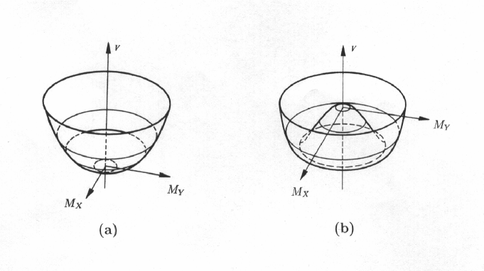
Figure 2.  : The potential $V(\vec{M})$ in the symmetric phase (a) and in the spontaneously broken phase (b)

There are two solutions for $\vec{M}$, depending on the value of $T$:

Solution I:

If $T>T_{C}\;\Rightarrow\left[\alpha_{1}(T-T_{C})+2\alpha_{2}(\vec{M}.\vec{M})\right]>0\;\Rightarrow\vec{M}=0$

The solution for $\vec{M}$ is the trivial one and corresponds to the situation I described before where the ground state is rotational invariant. The potential $V(\vec{M})$ has a symmetric shape with a unique minimum at the origen $\vec{M}=0$ where $V(0)=0$. This is represented in Fig.2a for the simplified bidimensional case, $\vec{M}=(M_{X},M_{Y})$.

Solution II:

If $T<T_{C}\;\Rightarrow\vec{M}=0$ is a local maximum and the condition of minimun requires:

$$\alpha_{1}(T-T_{C})+2\alpha_{2}(\vec{M}.\vec{M})=0\Rightarrow|\vec{M}|=\sqrt{\frac{\alpha_{1}(T_{C}-T)}{2\alpha_{2}}}$$

Namely, there are infinite absolute minima having all the same $|\vec{M}|$ above, but different direction of $\vec{M}$. This corresponds to the situation II where the system has infinite possible degenerate ground states which are not rotationally invariant. The potential $V(\vec{M})$ has a ’mexican hat shape’ as represented in Fig.2b for the bidimensional case.

Notice that it is the choice of the particular ground state what produces, for $T<T_{C}$, the spontaneous breaking of the rotational symmetry.

10.2 Spontaneous Symmetry Breaking in Quantum Field Theory: QCD as an example

In the language of Quantum Field Theory, a system is said to possess a symmetry that is spontaneously broken if the Lagrangian describing the dynamics of the system is invariant under these symmetry transformations, but the vacuum of the theory is not. Here the vacuum $|0>$ is the state where the Hamiltonian expectation value $<0|H|0>$ is minimum.

For illustrative purposes we present in the following the particular case of QCD where, besides the color gauge symmetry, there is an extra global symmetry, named chiral symmetry, which turns out to be spontaneously broken . For simplicity let us consider QCD with just two flavours. The Lagrangian is that in section 5 with just the two ligthest quarks, $u$ and $d$.

One can check that for $m_{u,d}=0$, ${\cal L}_{QCD}$ has the chiral symmetry $SU(2)_{L}\times SU(2)_{R}$ that is defined by the following transformations:

$$\Psi_{L}\rightarrow\Psi_{L}^{\prime}=U_{L}\Psi_{L}$$

$$\Psi_{R}\rightarrow\Psi_{R}^{\prime}=U_{R}\Psi_{R}$$

where,

$$\Psi=\left(\begin{array}[]{c}u\\ d\end{array}\right)\;;\;\Psi_{L}=\frac{1}{2}(1-\gamma_{5})\Psi\;;\;\Psi_{R}=\frac{1}{2}(1+\gamma_{5})\Psi$$

$$U_{L}\in SU(2)_{L}\;;\;U_{R}\in SU(2)_{R}$$

$U_{L}$ and $U_{R}$ can be written in terms of the 2x2 matrices $T_{L}^{a}$ and $T_{R}^{a}$ ($a=1,2,3$) corresponding to the generators $Q_{L}^{a}$ and $Q_{R}^{a}$ of $SU(2)_{L}$ and $SU(2)_{R}$ respectively:

$$U_{L}=\exp(-i\alpha_{L}^{a}T_{L}^{a})\;;\;U_{R}=\exp(-i\alpha_{R}^{a}T_{R}^{a})$$

It turns out that the physical vacuum of QCD is not invariant under the full chiral $SU(2)_{L}\times SU(2)_{R}$ group but just under the subgroup $SU(2)_{V}=SU(2)_{L+R}$ which is precisely the already introduced isospin group. The transformations given by the axial subgroup, $SU(2)_{A}$, do not leave the QCD vacuum invariant. Therefore, QCD with $m_{u,d}=0$ has a chiral symmetry which is spontaneously broken down to the isospin symmetry:

$$SU(2)_{L}\times SU(2)_{R}\rightarrow SU(2)_{V}$$

The fact that in Nature $m_{u,d}\neq 0$ introduces an extra explicit breaking of this chiral symmetry. Since the fermion masses are small this explicit breaking is soft. The chiral symmetry is not an exact but approximate symmetry of QCD.

One important question is still to be clarified. How do we know from experiment that, in fact, the QCD vacuum is not $SU(2)_{L}\times SU(2)_{R}$ symmetric?. Let us assume for the moment that it is chiral invariant. We will see that this assumption leads to a contradiction with experiment.

If $|0>$ is chiral invariant $\Rightarrow$

$$U_{L}|0>=|0>\;;\;U_{R}|0>=|0>\Rightarrow$$

$$T_{L}^{a}|0>=0;T_{R}^{a}|0>=0\Rightarrow Q_{L}^{a}|0>=0\;;\;Q_{R}^{a}|0>=0$$

In addition, if $|\Psi>$ is an eigenstate of the Hamiltonian and parity operator such that:

$$H|\Psi>=E|\Psi>\;;\;P|\Psi>=|\Psi>$$

then,

$$\exists|\Psi^{\prime}>=\frac{1}{\sqrt{2}}(Q_{R}^{a}-Q_{L}^{a})|\Psi>\;/\;H|\Psi^{\prime}>=E|\Psi^{\prime}>\;;\;P|\Psi^{\prime}>=-|\Psi^{\prime}>$$

In summary, if the QCD vacuum is chiral invariant there must exist pairs of degenerate states in the spectrum, the so-called parity doublets as $|\Psi>$ and $|\Psi^{\prime}>$, which are related by a chiral transformation and have opposite parities. The absence of such parity doublets in the hadronic spectrum indicates that the chiral symmetry must be spontaneously broken. Namely, there must exist some generators $Q^{a}$ of the chiral group such that $Q^{a}|0>\neq 0$. More specifically, it can be shown that these generators are the three $Q^{a}_{5}\;(a=1,2,3)$ of the axial group, $SU(2)_{A}$. In conclusion, the chiral symmetry breaking pattern in QCD is $SU(2)_{L}\times SU(2)_{R}\rightarrow SU(2)_{V}$ as announced.

10.3 Goldstone Theorem

One of the physical implications of the SSB phenomenom is the appearance of massless modes. For instance, in the case of the infinitely extended ferromagnet and below the Curie temperature there appear modes connecting the different possible ground states, the so-called spin waves.

The general situation in Quantum Fied Theory is described by the Goldstone Theorem [18]:

If a Theory has a global symmetry of the Lagrangian which is not a symmetry of the vacuum then there must exist one massless boson, scalar or pseudoscalar, associated to each generator which does not annihilate the vacuum and having its same quantum numbers. These modes are referred to as Nambu-Goldstone bosons or simply as Goldstone bosons.

Let us return to the example of QCD. The breaking of the chiral symmetry is characterized by $Q^{a}_{5}|0>\neq 0\;(a=1,2,3)$. Therefore, according to Goldstone Theorem, there must exist three massless Goldstone bosons, $\pi^{a}(x)\;\;a=1,2,3$, which are pseudoscalars. These bosons are identified with the three physical pions.

The fact that pions have $m_{\pi}\neq 0$ is a consequence of the soft explicit breaking in ${\cal L}_{QCD}$ given by $m_{q}\neq 0$. The fact that $m_{\pi}$ is small and that there is a large gap between this mass and the rest of the hadron masses can be seen as another manifestation of the spontaneous chiral symmetry breaking with the pions being the pseudo-Goldstone bosons of this breaking.

10.4 Dynamical Symmetry Breaking

In the previous sections we have seen the equivalence between the condition $Q^{a}|0>\neq 0$ and the non-invariance of the vacuum under the symmetry transformations generated by the $Q^{a}$ generators:

$$U|0>\neq|0>\;;\;U=\exp(i\epsilon^{a}Q^{a})$$

In Quantum Field Theory, it can be shown that an alternative way of characterizing the phenomenom of SSB is by certain field operators that have non-vanishing vacuum expectation values (v.e.v.).

$${\rm SSB}\Longleftrightarrow\exists\Phi_{j}/<0|\Phi_{j}|0>\neq 0$$

This non-vanishing v.e.v. plays the role of the order parameter signaling the existence of a phase where the symmetry of the vacuum is broken.

There are several possibilities for the nature of this field operator. In particular, when it is a composite operator which represents a composite state being produced from a strong underlying dynamics, the corresponding SSB is said to be a dynamical symmetry breaking. The chiral symmetry breaking in QCD is one example of this type of breaking. The non-vanishing chiral condensate made up of a quark and an anti-quark is the order paremeter in this case:

$$<0|\bar{q}q|0>\neq 0\Rightarrow SU(2)_{L}\times SU(2)_{R}\rightarrow SU(2)_{V}$$

The strong interactions of $SU(3)_{C}$ are the responsible for creating these $\bar{q}q$ pairs from the vacuum and, therefore, the $<0|\bar{q}q|0>$ should, in principle, be calculable from QCD.

It is interesting to mention that this type of symmetry breaking can happen similarly in more general $SU(N)$ gauge theories. The corresponding gauge couplings become sufficiently strong at large distances and allow for spontaneous breaking of their additional chiral-like symmetries. The corresponding order paremeter is also a chiral condensate: $<0|\overline{\Psi}\Psi|0>\neq 0$.

10.5 The Higgs Mechanism

The Goldstone Theorem is for theories with spontaneously broken global symmetries but does not hold for gauge theories. When a spontaneous symmetry breaking takes place in a gauge theory the so-called Higgs Mechanism operates [19]:

The would-be Goldstone bosons associated to the global symmetry breaking do not manifest explicitely in the physical spectrum but instead they ’combine’ with the massless gauge bosons and as result, once the spectrum of the theory is built up on the asymmetrical vacuum, there appear massive vector particles. The number of vector bosons that acquire a mass is precisely equal to the number of these would-be-Goldstone bosons.

There are three important properties of the Higgs Mechanism for ’mass generation’ that are worth mentioning:

• It respects the gauge symmetry of the Lagrangian.

• It preserves the total number of polarization degrees.

• It does not spoil the good high energy properties nor the renormalizability of the massless gauge theories.

We now turn to the case of the SM of Electroweak Interactions. We will see in the following how the Higgs Mechanism is implemented in the $SU(2)_{L}\times U(1)_{Y}$ Gauge Theory in order to generate a mass for the weak gauge bosons, $W^{\pm}$ and $Z$.

The following facts must be considered:

• The Lagrangian of the SM is gauge $SU(2)_{L}\times U(1)_{Y}$ symmetric. Therefore, anything we wish to add must preserve this symmetry.

• We wish to generate masses for the three gauge bosons $W^{\pm}$ and $Z$ but not for the photon, $\gamma$. Therefore, we need three would-be-Goldstone bosons, $\phi^{+}$, $\phi^{-}$ and $\chi$, which will combine with the three massless gauge bosons of the $SU(2)_{L}\times U(1)_{Y}$ symmetry.

• Since $U(1)_{em}$ is a symmetry of the physical spectrum, it must be a symmetry of the vacuum of the Electroweak Theory.

From the above considerations we conclude that in order to implement the Higgs Mechanism in the Electroweak Theory we need to introduce ’ad hoc’ an additional system that interacts with the gauge sector in a $SU(2)_{L}\times U(1)_{Y}$ gauge invariant manner and whose self-interactions, being also introduced ’ad hoc’, must produce the wanted breaking, $SU(2)_{L}\times U(1)_{Y}\rightarrow U(1)_{em}$, with the three associated would-be-Goldstone bosons $\phi^{+}$, $\phi^{-}$ and $\chi$. This sytem is the so-called SBS of the Electroweak Theory.

11 The Symmetry Breaking Sector of the Electroweak Theory

In this section we introduce and justify the simplest choice for the SBS of the Electroweak Theory.

Let $\Phi$ be the additional system providing the $SU(2)_{L}\times U(1)_{Y}\rightarrow U(1)_{em}$ breaking. $\Phi$ must fulfil the following conditions:

• It must be a scalar field so that the above breaking preserves Lorentz invariance.

• It must be a complex field so that the Hamiltonian is hermitian.

• It must have non-vanishing weak isospin and hypercharge in order to break $SU(2)_{L}$ and $U(1)_{Y}$. The assignment of quantum numbers and the choice of representation of $\Phi$ can be done in many ways. Some possibilities are:

  - Choice of a non-linear representation: $\Phi$ transforms non-linearly under $SU(2)_{L}\times U(1)_{Y}$.

  - Choice of a linear representation: $\Phi$ transforms linearly under $SU(2)_{L}\times U(1)_{Y}$. The simplest linear representation is a complex doublet. Alternative choices are: complex triplets, more than one doublet, etc. In particular, one may choose two complex doublets $H_{1}$ and $H_{2}$ as in the Minimal Supersymmetric SM.

• Only the neutral components of $\Phi$ are allowed to acquire a non-vanishing v.e.v. in order to preserve the $U(1)_{em}$ symmetry of the vacuum.

• The interactions of $\Phi$ with the gauge and fermionic sectors must be introduced in a gauge invariant way.

• The self-interactions of $\Phi$ given by the potential $V(\Phi)$ must produce the wanted breaking which is characterized in this case by $<0|\Phi|0>\neq 0$. $\Phi$ can be, in principle, a fundamental or a composite field.

• If we want to be predictive from low energies up to very high energies the interactions in $V(\Phi)$ must be renormalizable.

By taking into account the above seven points one is led to the following simplest choice for the system $\Phi$ and the Lagrangian of the SBS of the Electroweak Theory:

$${\cal L}_{SBS} = (D_{\mu}\Phi)^{\dagger}(D^{\mu}\Phi)-V(\Phi)$$

$$V(\Phi) = -\mu^{2}\Phi^{\dagger}\Phi+\lambda(\Phi^{\dagger}\Phi)^{2}\;;\;\lambda>0$$

where,

$$\Phi = \left(\begin{array}[]{c}\phi^{+}\\ \phi_{0}\end{array}\right)$$ (3)

$$D_{\mu}\Phi = (\partial_{\mu}-\frac{1}{2}ig\vec{\sigma}\cdot\vec{W}_{\mu}-\frac{1}{2}ig^{\prime}B_{\mu})\Phi$$

Here $\Phi$ is a fundamental complex doublet with hypercharge $Y(\Phi)=1$ and $V(\Phi)$ is the simplest renormalizable potential. $\vec{W}_{\mu}$ and $B_{\mu}$ are the gauge fields of $SU(2)_{L}$ and $U(1)_{Y}$ respectively and $g$ and $g^{\prime}$ are the corresponding gauge couplings.

It is interesting to notice the similarities with the Ginzburg-Landau Theory. Depending on the sign of the mass parameter ($-\mu^{2}$), there are two possibilities for the v.e.v. $<0|\Phi|0>$ that minimizes the potential $V(\Phi)$,

• $(-\mu^{2})>0$: The minimum is at:

  $$<0|\Phi|0>=0$$

  The vacuum is $SU(2)_{L}\times U(1)_{Y}$ symmetric and therefore no symmetry breaking occurs.

• $(-\mu^{2})<0$: The minimum is at:

  $$|<0|\Phi|0>|=\left(\begin{array}[]{c}0\\ \frac{v}{\sqrt{2}}\end{array}\right)\;\;;\;\;{\rm arbitrary}\;\;arg\;\Phi\;\;;\;\;v\equiv\sqrt{\frac{\mu^{2}}{\lambda}}$$

  Therefore, there are infinite degenerate vacua corresponding to infinite posssible values of $arg\;\Phi$. Either of these vacua is $SU(2)_{L}\times U(1)_{Y}$ non-symmetric and $U(1)_{em}$ symmetric. The breaking $SU(2)_{L}\times U(1)_{Y}\rightarrow U(1)_{em}$ occurs once a particular vacuum is chosen. As usual, the simplest choice is taken:

  $$|<0|\Phi|0>|=\left(\begin{array}[]{c}0\\ \frac{v}{\sqrt{2}}\end{array}\right)\;;\;arg\;\Phi\equiv 0\;;\;v\equiv\sqrt{\frac{\mu^{2}}{\lambda}}$$

The two above symmetric and non-symmetric phases of the Electroweak Theory are clearly similar to the two phases of the ferromagnet that we have described within the Ginzburg Landau Theory context. In the SM, the field $\Phi$ replaces the magnetization $\vec{M}$ and the potential $V(\Phi)$ replaces $V(\vec{M})$. The SM order papameter is, consequently, $<0|\Phi|0>$. In the symmetric phase, $V(\Phi)$ is as in Fig.2a, whereas in the non-symmetric phase, it is as in Fig.2b.

Another interesting aspect of the Higgs Mechanism, as we have already mentioned, is that it preserves the total number of polarization degrees. Let us make the counting in detail:

• Before SSB
  4 massless gauge bosons: $W^{\mu}_{1,2,3},B^{\mu}$
  4 massless scalars: The 4 real components of $\Phi$: $\phi_{1},\phi_{2},\phi_{3},\phi_{4}$
  

  Total number of polarization degrees $=4\times 2+4=12$

• After SSB
  3 massive gauge bosons: $W^{\pm},Z$
  1 massless gauge boson: $\gamma$
  1 massive scalar: $H$
  

  Total number of polarization degrees: $3\times 3+1\times 2+1=12$

Furthermore, it is important to realize that one more degree than needed is introduced into the theory from the beginning. Three of the real components of $\Phi$, or similarly $\phi^{\pm}\equiv\frac{1}{\sqrt{2}}(\phi_{1}\mp i\phi_{2})$ and $\chi=\phi_{3}$, are the needed would-be Goldstone bosons and the fourth one $\phi_{4}$ is introduced just to complete the complex doublet. After the symmetry breaking, this extra degree translates into the apparition in the spectrum of an extra massive scalar particle , the Higgs boson particle $H$.

12 Lagrangian of The Electroweak Theory II

In order to get the particle spectra and the particle masses we first rewrite the full SM Lagrangian which is $SU(2)_{L}\times U(1)_{Y}$ gauge invariant:

$${\cal L}_{SM} = {\cal L}_{f}+{\cal L}_{G}+{\cal L}_{SBS}+{\cal L}_{YW}$$

where, ${\cal L}_{f}$, and ${\cal L}_{G}$ have been given previously and ${\cal L}_{SBS}$ and ${\cal L}_{YW}$ are the SBS and the Yukawa Lagrangians respectively,

${\cal L}_{SBS}=(D_{\mu}\Phi)^{\dagger}(D^{\mu}\Phi)+\mu^{2}\Phi^{\dagger}\Phi-\lambda(\Phi^{\dagger}\Phi)^{2}$ ${\cal L}_{YW}=\lambda_{e}\bar{l}_{L}\Phi e_{R}+\lambda_{u}\bar{q}_{L}\widetilde{\Phi}u_{R}+\lambda_{d}\bar{q}_{L}\Phi d_{R}+h.c.+2^{nd}\;{\rm and}\;3^{rd}\;{\rm families}$

Here,

$$l_{L} = \left(\begin{array}[]{c}\nu_{L}\\ e_{L}\end{array}\right)\;;\;\;q_{L}=\left(\begin{array}[]{c}u_{L}\\ d_{L}\end{array}\right)$$ (8)

$$\Phi = \left(\begin{array}[]{c}\phi^{+}\\ \phi_{0}\end{array}\right)\;;\;\;\widetilde{\Phi}=i\sigma_{2}\Phi^{*}=\left(\begin{array}[]{c}\phi^{*}_{0}\\ -\phi^{-}\end{array}\right)$$ (13)

Notice that ${\cal L}_{SBS}$ is needed to provide the $M_{W}$ and $M_{Z}$ masses and ${\cal L}_{YW}$ is needed to provide the $m_{f}$ masses.

The following steps summarize the procedure to get the spectrum from ${\cal L}_{SM}$:

• A non-symmetric vacuum must be fixed. Let us choose, for instance,

  $$<0|\Phi|0>=\left(\begin{array}[]{c}0\\ \frac{v}{\sqrt{2}}\end{array}\right)$$

• The physical spectrum is built by performing ’small oscillations’ around this vacuum. These are parametrized by,

  $$\Phi(x)=\exp{\left(i\frac{\vec{\xi}(x)\vec{\sigma}}{v}\right)}\left(\begin{array}[]{c}0\\ \frac{v+H(x)}{\sqrt{2}}\end{array}\right)$$

  where $\vec{\xi}(x)$ and $H(x)$ are ’small’ fields.

• In order to eliminate the unphysical fields $\vec{\xi}(x)$ we make the following gauge transformations:

  $$\Phi^{\prime} = U(\xi)\Phi=\left(\begin{array}[]{c}0\\ \frac{v+H}{\sqrt{2}}\end{array}\right)\;;\;U(\xi)=\exp\left(-i\frac{\vec{\xi}\vec{\sigma}}{v}\right)$$ (16)

  $$l_{L}^{\prime} = U(\xi)l_{L}\;;\;e_{R}^{\prime}=e_{R}\;;\;q_{L}^{\prime}=U(\xi)q_{L}\;;\;u_{R}^{\prime}=u_{R}\;;\;d_{R}^{\prime}=d_{R}$$

  $$\left(\frac{\vec{\sigma}\cdot\vec{W}^{\prime}_{\mu}}{2}\right) = U(\xi)\left(\frac{\vec{\sigma}\cdot\vec{W}_{\mu}}{2}\right)U^{-1}(\xi)-\frac{i}{g}(\partial_{\mu}U(\xi))U^{-1}(\xi)\;;\;B^{\prime}_{\mu}=B_{\mu}$$

• Finally, the weak eigenstates are rotated to the mass eigenstates which define the physical gauge boson fields:

  $$W^{\pm}_{\mu} = \frac{W^{\prime 1}_{\mu}\mp iW^{\prime 2}_{\mu}}{\sqrt{2}},$$

  $$Z_{\mu} = c_{w}W^{\prime 3}_{\mu}-s_{w}B^{\prime}_{\mu},$$

  $$A_{\mu} = s_{w}W^{\prime 3}_{\mu}+c_{w}B^{\prime}_{\mu},$$

It is now straightforward to read the masses from the following terms of ${\cal L}_{SM}$:

$$(D_{\mu}\Phi^{\prime})^{\dagger}(D^{\mu}\Phi^{\prime}) = \left(\frac{g^{2}v^{2}}{4}\right)W^{+}_{\mu}W^{\mu-}+\frac{1}{2}\left(\frac{(g^{2}+g^{\prime 2})v^{2}}{4}\right)Z_{\mu}Z^{\mu}+...$$

$$V(\Phi^{\prime}) = \frac{1}{2}(2\mu^{2})H^{2}+...$$

$${\cal L}_{YW} = \left(\lambda_{e}\frac{v}{\sqrt{2}}\right)\bar{e}^{\prime}_{L}e^{\prime}_{R}+\left(\lambda_{u}\frac{v}{\sqrt{2}}\right)\bar{u}^{\prime}_{L}u^{\prime}_{R}+\left(\lambda_{d}\frac{v}{\sqrt{2}}\right)\bar{d}^{\prime}_{L}d^{\prime}_{R}+...$$

and get finally the tree level predictions:

$$M_{W} = \frac{gv}{2}\;;\;M_{Z}=\frac{\sqrt{g^{2}+g^{\prime 2}}v}{2}$$

$$M_{H} = \sqrt{2}\mu$$

$$m_{e} = \lambda_{e}\frac{v}{\sqrt{2}}\;;\;m_{u}=\lambda_{u}\frac{v}{\sqrt{2}}\;;\;m_{d}=\lambda_{d}\frac{v}{\sqrt{2}}\;;...$$

where,

$$v=\sqrt{\frac{\mu^{2}}{\lambda}}$$

Finally one can rewrite ${\cal L}_{SBS}$ and ${\cal L}_{YW}$, after the application of the Higgs Mechanism, in terms of the physical scalar fields, and get not just the mass terms but also the kinetic and interaction terms for the Higgs sector,

$${\cal L}_{SBS}+{\cal L}_{YW}\rightarrow{\cal L}_{H}^{\rm free}+{\cal L}_{H}^{\rm int}+...$$

where,

${\cal L}_{H}^{\rm free}=\frac{1}{2}\partial_{\mu}H\partial^{\mu}H-\frac{1}{2}M_{H}^{2}H^{2}$

and,

${\cal L}_{H}^{\rm int}=-\frac{M_{H}^{2}}{2v}H^{3}-\frac{M_{H}^{2}}{8v^{2}}H^{4}$ $\;\;\;\;-\frac{m_{f}}{v}\overline{f}Hf$ $\;\;\;\;+M_{W}^{2}W_{\mu}^{+}W^{\mu\;-}\left(1+\frac{2}{v}H+\frac{1}{v^{2}}H^{2}\right)$ $\;\;\;\;+\frac{1}{2}M_{Z}^{2}Z_{\mu}Z^{\mu}\left(1+\frac{2}{v}H+\frac{1}{v^{2}}H^{2}\right)$

Some comments are in order.

• All masses are given in terms of a unique mass parameter $v$ and the couplings $g$, $g^{\prime}$, $\lambda$, $\lambda_{e}$, etc..

• The interactions of $H$ with fermions and with gauge bosons are proportional to the gauge couplings and to the corresponding particle masses:

  $$f\bar{f}H\;:\;-i\frac{g}{2}\frac{m_{f}}{M_{W}}\;;\;\;\;W^{+}_{\mu}W^{-}_{\nu}H\;:\;igM_{W}g_{\mu\nu}\;;\;\;\;Z_{\mu}Z_{\nu}H\;:\;\frac{ig}{c_{w}}M_{Z}g_{\mu\nu}$$

• The v.e.v. $v$ is determined experimentally form $\mu$-decay. By identifying the predictions of the partial width $\Gamma(\mu\rightarrow\nu_{\mu}\bar{\nu}_{e}e)$ in the SM to low energies ($q^{2}<<M_{W}^{2}$) and in the V-A Theory one gets,

  $$\frac{G_{F}}{\sqrt{2}}=\frac{g^{2}}{8M_{W}^{2}}=\frac{1}{2v^{2}}$$

  And from here,

  $$v=(\sqrt{2}G_{F})^{-\frac{1}{2}}=246\;GeV$$

• The values of $M_{W}$ and $M_{Z}$ were anticipated successfully quite before they were measured in experiment. The input parameters were $\theta_{w}$, the fine structure constant $\alpha$ and $G_{F}$. Before LEP these were the best measured electroweak parameters.

• In contrast to the gauge boson sector, the Higgs boson mass $M_{H}$ and the Higgs self-coupling $\lambda$ are completely undetermined in the SM. They are related at tree level by, $\lambda=\frac{M_{H}^{2}}{2v^{2}}$.

• The hierarchy in the fermion masses is also completely undetermined in the SM.

13 Theoretical Bounds on $M_{H}$

In this section we summarize the present bounds on $M_{H}$ from the requirement of consistency of the theory.

13.1 Upper bound on $M_{H}$ from Unitarity

Unitarity of the scattering matrix together with the elastic approximation for the total cross-section and the Optical Theorem imply certain elastic unitarity conditions for the partial wave amplitudes. These, in turn, when applied in the SM to scattering processes involving the Higgs particle, imply an upper limit on the Higgs mass. Let us see this in more detail for the simplest case of scattering of massless scalar particles: $1+2\rightarrow 1+2$.

The decomposition of the amplitude in terms of partial waves is given by:

$$T(s,\cos\theta) = 16\pi\sum_{J=0}^{\infty}(2J+1)a_{J}(s)P_{J}(\cos\theta)$$

where $P_{J}$ are the Legendre polynomials.

The corresponding differential cross-section is given by:

$$\frac{d\sigma}{d\Omega} = \frac{1}{64\pi^{2}s}|T|^{2}$$

Thus, the elastic cross-section is written in terms of partial waves as:

$$\sigma_{\rm el} = \frac{16\pi}{s}\sum_{J=0}^{\infty}(2J+1)|a_{J}(s)|^{2}$$

On the other hand, the Optical Theorem relates the total cross-section with the forward elastic scattering amplitude:

$$\sigma_{\rm tot}(1+2\rightarrow{\rm anything}) = \frac{1}{s}Im\;T(s,\cos\theta=1)$$

In the elastic approximation for $\sigma_{\rm tot}$ one gets $\sigma_{\rm tot}\approx\sigma_{\rm el}$. From this one finally finds,

$$Im\;a_{J}(s) = |a_{J}(s)|^{2}\;;\;\forall J$$

This is called the elastic unitariry condition for partial wave amplitudes. It is easy to get from this the following inequalities:

$$|a_{J}|^{2}\leq 1\;;\;0\leq Im\;a_{J}\leq 1\;;\;|Re\;a_{J}|\leq\frac{1}{2}\;;\;\forall J$$

These are necessary but not sufficient conditions for elastic unitarity. It implies that if any of them are not fulfiled then the elastic unitarity condition also fails, in which case the unitarity of the theory is said to be violated.

Let us now study the particular case of $W_{L}^{+}W_{L}^{-}$ scattering in the SM and find its unitarity conditions. The $J=0$ partial wave can be computed from:

$$a_{0}(W_{L}^{+}W_{L}^{-}\rightarrow W_{L}^{+}W_{L}^{-}) = \frac{1}{32\pi}\int_{-1}^{1}T(s,\cos\theta)d(\cos\theta)$$

where the amplitude $T(s,\cos\theta)$ is given by,

$$T(W_{L}^{+}W_{L}^{-}\rightarrow W_{L}^{+}W_{L}^{-}) = -\frac{1}{v^{2}}\{-s-t+\frac{s^{2}}{s-M_{H}^{2}}+\frac{t^{2}}{t-M_{H}^{2}}+2M_{Z}^{2}+$$

$$\frac{2M_{Z}^{2}s}{t-M_{Z}^{2}}+\frac{2t}{s}(M_{Z}^{2}-4M_{W}^{2})-\frac{8s_{W}^{2}M_{W}^{2}M_{Z}^{2}s}{t(t-M_{Z}^{2})}\}$$

By studying the large energy limit of $a_{0}$ one finds,

$$|a_{0}| \stackrel{{\scriptstyle s>>M_{H}^{2},M_{V}^{2}}}{{\longrightarrow}} \frac{M_{H}^{2}}{8\pi v^{2}}$$

Finally, by requiring the unitarity condition $|Re\;a_{0}|\leq\frac{1}{2}$ one gets the following upper bound on the Higgs mass:

$$M_{H}<860\;GeV$$

One can repeat the same reasoning for different channels and find similar or even tighter bounds than this one [31, 32].

At this point, it should be mentioned that these upper bounds based on perturbative unitarity do not mean that the Higgs particle cannot be heavier than these values. The conclusion should be, instead, that for those large $M_{H}$ values a perturbative approach is not valid and non-perturbative techniques are required. In that case, the Higgs self-interactions governed by the coupling $\lambda$ become strong and new physics phenomena may appear in the $O(1\;TeV)$ range. In particular, the scattering of longitudinal gauge bosons may also become strong in that range [31] and behave similarly to what happens in $\pi\pi$ scattering in the $O(1\;GeV)$ range. Namely, there could appear new resonances, as it occurs typically in a theory with strong interactions. This new interesting phenomena could be studied at the next hadron collider, LHC [31, 33].

13.2 Upper bound on $M_{H}$ from Triviality

Triviality in $\lambda\Phi^{4}$ theories [34] (as, for instance, the scalar sector of the SM) means that the particular value of the renormalized coupling of $\lambda_{R}=0$ is the unique fixed point of the theory. A theory with $\lambda_{R}=0$ contains non-interacting particles and therefore it is trivial. This behaviour can already be seen in the renormalized coupling at one-loop level:

$$\lambda_{R}(Q) = \frac{\lambda_{0}}{1-\frac{3}{2\pi^{2}}\lambda_{0}\log(\frac{Q}{\Lambda})}\;;\;\lambda_{0}\equiv\lambda_{R}(Q=\Lambda)$$

As we attempt to remove the cut-off $\Lambda$ by taking the limit $\Lambda\rightarrow\infty$ while $\lambda_{0}$ is kept fixed to an arbitrary but finite value, we find out that $\lambda_{R}(Q)\rightarrow 0$ at any finite energy value $Q$. This, on the other hand, can be seen as a consequence of the existence of the well known Landau pole of $\lambda\Phi^{4}$ theories.

The trivilaty of the SBS of the SM is cumbersome since we need a self-interacting scalar system to generate $M_{W}$ and $M_{Z}$ by the Higgs Mechanism. The way out from this apparent problem is to assume that the Higgs potential $V(\Phi)$ is valid just below certain ’physical’ cut-off $\Lambda_{\rm phys}$. Then, $V(\Phi)$ describes an effective low energy theory which emerges from some (so far unknown) fundamental physics with $\Lambda_{\rm phys}$ being its characteristics energy scale. We are going to see next that this assumption implies an upper bound on $M_{H}$ [35].

Let us assume some concrete renormalization of the SM parameters. The conclusion does not depend on this particular choice. Let us define, for instance, the renormalized Higgs mass parameter as:

$$M_{H}^{2} = 2\lambda_{R}(v)v^{2}$$

where,

$$\lambda_{R}(v) = \frac{\lambda_{0}}{1-\frac{3}{2\pi^{2}}\lambda_{0}\log(\frac{v}{\Lambda_{\rm phys}})}$$

Now, if we want $V(\Phi)$ to be a sensible effective theory, we must keep all the renormalized masses below the cut-off and, in particular, $M_{H}<\Lambda_{\rm phys}$. However, one can see that for arbitrary values of $\Lambda_{\rm phys}$ it is not always possible. By increasing the value of $\Lambda_{\rm phys}$, $M_{H}$ decreases and the other way around, by lowering $\Lambda_{\rm phys}$, $M_{H}$ grows. There is a crossing point where $M_{H}\approx\Lambda_{\rm phys}$ which happens to be around an energy scale of approximately $1\;TeV$. Since we want to keep the Higgs mass below the physical cut-off, it implies finally the announced upper bound,

$$M_{H}^{\rm 1-loop}<1\;TeV$$

Of course, this should be taken just as a perturbative estimate of the true triviality bound. A more realistic limit must come from a non-perturbative treatment. In particular, the analyses performed on the lattice [36] confirm this behaviour and place even tighter limits. The following bound is found,

$$M_{H}^{\rm Lattice}<640\;GeV$$

Finally, a different but related perturbative upper limit on $M_{H}$ can be found by analysing the renormalization group equations in the SM to one-loop. Here one includes, the scalar sector, the gauge boson sector and restricts the fermionic sector to the third generation. By requiring the theory to be perturbative (i.e. all the couplings be sufficiently small) at all the energy scales below some fixed high energy, one finds a maximum allowed $M_{H}$ value [37]. For instance, by fixing this energy scale to $10^{16}\;GeV$ and for $m_{t}=170\;GeV$ one gets:

$$M_{H}^{\rm RGE}<170\;GeV$$

Of course to believe in perturbativity up to very high energies could be just a theoretical prejudice. The existence of a non-perturbative regime for the scalar sector of the SM is still a possibility and one should be open to new proposals in this concern.

13.3 Lower bound on $M_{H}$ from Vacuum Stability

Once the asymmetric vacuum of the $SU(2)_{L}\times U(1)_{Y}$ theory has been fixed, one must require this vacuum to be stable under quantum corrections. In principle, quantum corrections could destabilize the asymmetric vacuum and change it to the symmetric one where the SSB does not take place. This phenomenom can be better explained in terms of the effective potential with quantum corrections included. Let us take, for instance, the effective potential of the Electroweak Theory to one loop in the small $\lambda$ limit:

$$V_{\rm eff}^{\rm 1-loop}(\Phi) \simeq -\mu^{2}\Phi^{\dagger}\Phi+\lambda_{R}(Q_{0})(\Phi^{\dagger}\Phi)^{2}+\beta_{\lambda}(\Phi^{+}\Phi)^{2}\log\left(\frac{\Phi^{\dagger}\Phi}{Q_{0}^{2}}\right)$$

where, $\beta_{\lambda}\equiv\frac{d\lambda}{dt}\simeq\frac{1}{16\pi^{2}}\left[-3\lambda_{t}^{4}+\frac{3}{16}(2g^{4}+(g^{2}+g^{\prime 2})^{2})\right]$.

The condition of extremum is:

$$\frac{\delta V_{\rm eff}^{\rm 1-loop}}{\delta\Phi} = 0$$

which leads to two possible solutions: a) The trivial vacuum with $\Phi=0$; and b) The non-trivial vacuum with $\Phi=\Phi_{\rm vac}\neq 0$. If we want the true vacuum to be the non-trivial one we must have:

$$V_{\rm eff}^{\rm 1-loop}(\Phi_{\rm vac}) < V_{\rm eff}^{\rm 1-loop}(0)$$

However, the value of the potential at the minimum depends on the size of its second derivative:

$$M_{H}^{2}\equiv\frac{1}{2}\{\frac{\delta^{2}V}{\delta\Phi^{2}}\}_{\Phi=\Phi_{\rm vac}}$$

and, it turns out that for too low values of $M_{H}^{2}$ the condition above turns over. That is, $V(0)<V(\Phi_{\rm vac})$ and the true vacuum changes to the trivial one. The condition for vacuum stability then implies a lower bound on $M_{H}$ [38]. More precisely,

$$M_{H}^{2} > \frac{3}{16\pi^{2}v^{2}}(2M_{W}^{4}+M_{Z}^{4}-4m_{t}^{4})$$

Surprisingly, for $m_{t}>78\;GeV$ this bound dissapears and, moreover, $V_{\rm eff}^{\rm 1-loop}$ becomes unbounded from below!. Apparently it seems a disaster since the top mass is known at present and is certainly larger than this value. The solution to this problem relies in the fact that for such input values, the 1-loop approach becomes unrealistic and a 2-loop analysis of the effective potential is needed. Recent studies indicate that by requiring vacuum stability at 2-loop level and up to very large energies of the order of $10^{16}\;GeV$, the following lower bound is found [39]:

$$M_{H}^{\rm v.stab.} > 132\;GeV$$

This is for $m_{t}=170\;GeV$ and $\alpha_{s}=0.117$ and there is an uncertainty in this bound of $5$ to $10$ $GeV$ from the uncertainty in the $m_{t}$ and $\alpha_{s}$ values.

14 SM predictions

In the following we present the tree level predictions from the SM and compare them with the present experimental values. The experimental values presented here (unless explicitely stated otherwise) have been borrowed from the talk by D.Karlen given at the ICHEP’98 Vancouver Conference [4]. For a more detailed discussion on the experimental tests of the SM see the lectures of L. Nodulman.

14.1 Gauge Boson Masses

Before the discovery of the $W^{\pm}$, $Z$ gauge bosons, the best known SM parameters were $\alpha$, $G_{F}$ and $sin^{2}\theta_{w}$. The present values are highly precise:

$$\alpha^{-1}_{exp}=137.0359895\pm 0.0000061$$

from atomic, molecular and nuclear data, and

$$G_{F}^{exp}=(1.16639\pm 0.000022)\times 10^{-5}\;GeV^{-2}$$

from $\mu-$decay.
$sin^{2}\theta_{w}$ was measured firstly in the seventies in $\nu N$ scattering experiments. The ratio of the cross-sections for neutral currents and charged currents as predicted in the SM is a known function of $sin\theta_{w}$,

$$\frac{\sigma_{NC}(\nu q\rightarrow\nu q)}{\sigma_{CC}(\nu q\rightarrow lq^{\prime})}\sim f(sin^{2}\theta_{w})$$

It is the measurement of this ratio what provides a measurement of $sin^{2}\theta_{w}$. The present experimental value is,

$$sin^{2}\theta_{w}|_{\rm exp}=0.2255\pm 0.0021$$

The SM does not predict a numerical value for $M_{W}$ and $M_{Z}$ but provides some relations among the relevant parameters. These relations are different to tree level than to, for instance, one-loop level. In particular, the following relations hold to tree level in the SM,

$$M_{W}=\frac{gv}{2}\;;\frac{G_{F}}{\sqrt{2}}=\frac{g^{2}}{8M_{W}^{2}}=\frac{1}{2v^{2}}\;;\;g=\frac{e}{s_{w}}\;;\;\rho_{SM}^{\rm tree}\equiv\frac{M_{W}^{2}}{M_{Z}^{2}c_{w}^{2}}=1$$

From these expressions it is inmediate to derive the two following tree level relations,

$$M_{W}=\left(\frac{\pi\alpha}{G_{F}\sqrt{2}}\right)^{\frac{1}{2}}\frac{1}{sin\theta_{w}}$$

$$M_{Z}=\left(\frac{\pi\alpha}{G_{F}\sqrt{2}}\right)^{\frac{1}{2}}\frac{1}{sin\theta_{w}cos\theta_{w}}$$

Finally, by inserting the experimental values of $\alpha$, $G_{F}$ and $\theta_{w}$ into these expressions one gets the tree level values for the gauge boson masses,

$$M_{W}^{\rm tree}=78\;GeV\;\;;\;\;M_{Z}^{\rm tree}=89\;GeV$$

The discovery of the $W^{\pm}$ and $Z$ gauge bosons in 1983 at the CERN $SpS$ collider [30] lead to the definitive confirmation of the validity of the SM. Notice that the measured masses were surprisingly close to the SM tree level predictions,

$$M_{W}^{\rm SpS}=(81\pm 2)\;GeV\;\;;\;\;M_{Z}^{\rm SpS}=(93\pm 3)\;GeV$$

The present experimental values are very precise,

$$M_{W}^{\rm exp} = (80.41\pm 0.09)\;GeV\;(p\overline{p})$$

$$(80.37\pm 0.09)\;GeV\;({\rm LEP})$$

$$M_{Z}^{\rm exp} = (91.1867\pm 0.0021)\;GeV\;({\rm LEP})$$

14.2 Gauge Boson Decays

The $W^{\pm}$ and $Z$ gauge bosons can decay either in quarks or in leptons within the SM. The dominant decays are clearly into quarks due to the extra color factor, $N_{C}$, which is not present in the leptonic decays. The tree level predictions for the partial widths in the approximation of neglecting the fermion masses are the following,

$$\Gamma(W^{+}\rightarrow e^{+}\nu_{e})=\frac{g^{2}}{48\pi}M_{W}=\frac{G_{F}M_{W}^{3}}{6\sqrt{2}\pi}=0.232\;GeV$$

$$\Gamma(W^{+}\rightarrow\mu^{+}\nu_{\mu})=\Gamma(W^{+}\rightarrow\tau^{+}\nu_{\tau})=\Gamma(W^{+}\rightarrow e^{+}\nu_{e})$$

$$\Gamma(W^{+}\rightarrow u_{i}\overline{d}_{j})=N_{C}|U_{ij}|^{2}\frac{G_{F}M_{W}^{3}}{6\sqrt{2}\pi}=0.232\;N_{C}|U_{ij}|^{2}\;GeV$$

$$\Gamma(Z\rightarrow f\overline{f})=\kappa_{f}\frac{G_{F}M_{Z}^{3}}{6\sqrt{2}\pi}(g_{Vf}^{2}+g_{Af}^{2})=0.3318\kappa_{f}(g_{Vf}^{2}+g_{Af}^{2})\;GeV$$

where, $U_{ij}$ are the CKM matrix elements and,

$$\kappa_{f}=1\;,\;f=l,\nu\;;\;\kappa_{f}=N_{C}\;,\;f=q\;;\;g_{Vf}=T^{f}_{3}-2Q^{f}s_{w}^{2}\;;\;g_{Af}=T^{f}_{3}$$

In Table 3 it is shown the tree level predictions in the SM, for the total $Z$ and $W^{\pm}$ widths, $\Gamma_{Z}$ and $\Gamma_{W}$, and the ratios:

$$R_{e}=\frac{\Gamma(Z\rightarrow{\rm hadrons})}{\Gamma_{e}}\;;\;R_{b}=\frac{\Gamma(Z\rightarrow b\overline{b})}{\Gamma(Z\rightarrow{\rm hadrons})}\;;\;R_{c}=\frac{\Gamma(Z\rightarrow c\overline{c})}{\Gamma(Z\rightarrow{\rm hadrons})}$$

The numerical predictions shown here use as input the present experimental values for $M_{Z}$, $G_{F}$, $\alpha$ and $sin^{2}\theta_{w}$, and the $M_{W}$ value that one gets with those experimental values put into the previous SM tree level relation. That is, $M_{W}=80.94\;GeV$.

TABLE 3.  : Confronting tree level SM predictions with data

 Parameter Tree Level SM Exp. value  $\Gamma_{Z}(GeV)$ $2.474$ $2.4948\pm 0.0025$ $\Gamma_{W}(GeV)$ $2.09$ $2.06\pm 0.06$ $R_{e}$ $20.29$ $20.765\pm 0.026$ $R_{b}$ $0.219$ $0.21656\pm 0.00074$ $R_{c}$ $0.172$ $0.1733\pm 0.0044$  

By comparing the tree level SM results with the present experimental values it is clear that they provide reasonable good predictions. However, due to the high level of precision of the present measurements one can also conclude from this table that some of the tree level predictions are already not compatible with data. In fact in some observables they are out by several standard deviations. This is a clear indication that the SM radiative corrections must be included in the theoretical predictions [40]. The present experimental analysis of the SM parameters, in fact, do include these radiative corrections. The summary of measurements included in the combined analysis of SM parameters from LEP and SLC can be found in Nodulman lectures.

14.3 Top Quark Physics

As has been shown before, the top mass $m_{t}$ is not predicted in the SM. Instead, the SM provides, via The Higgs Mechanism, the tree level relation,

$$m_{t}=\lambda_{t}\frac{v}{\sqrt{2}}=\lambda_{t}\left(\frac{1}{2\sqrt{2}G_{F}}\right)^{\frac{1}{2}}$$

which gives $m_{t}$ in terms of the top Yukawa coupling $\lambda_{t}$. But, $\lambda_{t}$ as the other fermion Yukawa couplings are unknown parameters in the SM.

Figure 3.  : $t\overline{t}$ production at hadron colliders

The existence of the top quark, however, was never questioned seriously, since there were several strong arguments supporting the need of this third generation fermion. On one hand, the top quark was needed to avoid unwanted flavour changing neutral currents (FCNC). On the other hand the top quark was needed to avoid unwanted $SU(2)_{L}\times U(1)_{Y}$ anomalies. Thus, The top quark was expected for a long time. Its discovery finally occured in 1994 at the $p\overline{p}$ TeVatron collider at Fermilab [27]. The present experimental value of the top mass as provided by the two Tevatron experiments is,

$$m_{t}^{\rm exp}=(173.8\pm 5.0)\;GeV\;({\rm CDF}+{\rm D}0)$$

It is remarkable this much larger mass value than the rest of the fermion masses. In fact, for this top mass value one can extract the corresponding Yukawa coupling and get $\lambda_{t}\sim 1$ which is a rather large value, although it can still be considered as a perturbative coupling. To the question, why the top quark is so heavy?, there is no answer within the SM.

Concerning the top quark decays, the dominant one is by far the decay into a $W^{+}$ gauge boson and a bottom quark. The SM tree level prediction for the partial width, in the approximation of neglecting $m_{b}$, is

$$\Gamma(t\rightarrow W^{+}b)=\frac{G_{F}m_{t}^{3}}{8\pi\sqrt{2}}|U_{tb}|^{2}\left(1-\frac{M_{W}^{2}}{m_{t}^{2}}\right)\left(1+2\frac{M_{W}^{2}}{m_{t}^{2}}\right)\sim 2\;GeV$$

There is not experimental meassurement of the total or partial width yet.

Regarding the top production, it is obvious that, given the large mass value, it can only be produced at present in the TeVatron collider. The future hadron collider LHC at CERN will provide additional interesting information on top quark physics. In Figure 3 it is shown the cross-section for $t\overline{t}$ production at TeVatron and LHC from the various possible channels. It is clear from the figure that $q\overline{q}\rightarrow t\overline{t}$ is the dominant process at TeVatron, whereas $gg\rightarrow t\overline{t}$ will dominate at LHC [41].

14.4 Higgs Physics

The Higgs mass $M_{H}$ is not predicted in the SM either. The Higgs Mechanism provides $M_{H}$ as a function of the Higgs self-coupling $\lambda$ and $v=246\;GeV$,

$$M_{H}=\sqrt{2}\mu=\sqrt{2v^{2}\lambda}$$

but, $\lambda$ is also unknown. Therefore, $M_{H}$ can take any value in the SM. As we have seen, the unique restrictions on $M_{H}$ come from the consistency of the theory, that is from unitarity, triviality, and vacuum stability arguments.

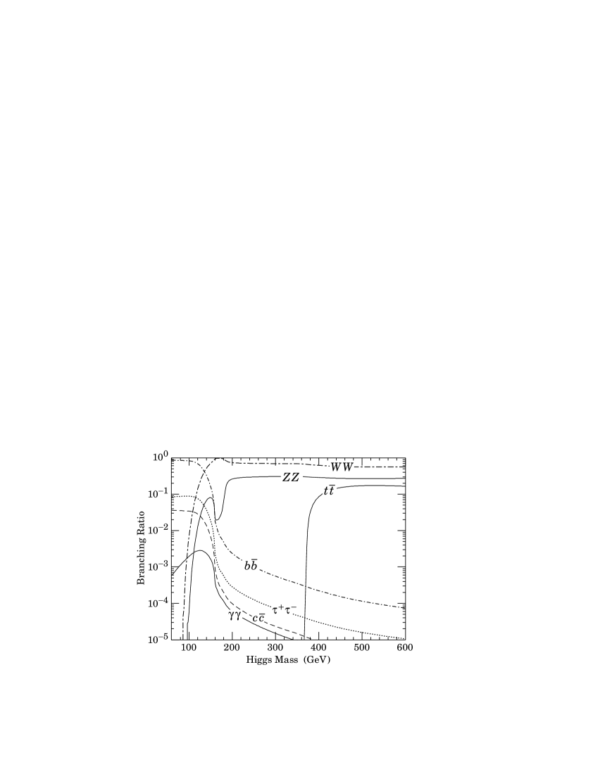
Figure 4.  : Branching ratios for Higgs decays as a function of $M_{H}$

Contrary to the top quark case, there are no strong theoretical arguments (anomalies, etc) supporting the need of this scalar elementary particle, $H$.

Regarding the Higgs decays, the tree level SM predictions for the partial widths are the following,

$$\Gamma(H\rightarrow W^{+}W^{-})=\frac{G_{F}M_{H}^{3}}{8\sqrt{2}\pi}\beta_{W}\left(\beta_{W}^{2}+\frac{12M_{W}^{4}}{M_{H}^{4}}\right)$$

$$\Gamma(H\rightarrow ZZ)=\frac{G_{F}M_{H}^{3}}{16\sqrt{2}\pi}\beta_{Z}\left(\beta_{Z}^{2}+\frac{12M_{Z}^{4}}{M_{H}^{4}}\right)$$

$$\Gamma(H\rightarrow f\overline{f})=\frac{G_{F}m_{f}^{2}M_{H}}{4\sqrt{2}\pi}\beta_{f}^{3}\xi$$

where,

$$\beta_{P}=\sqrt{1-4\frac{m_{P}^{2}}{M_{H}^{2}}}\;,\;P=W^{\pm},Z,f\;\;;\;\;\xi=3\;{\rm if}\;f=q\;,\;\xi=1\;{\rm if}\;f=l$$

In Figure 4 there are shown the Higgs branching ratios as a function of the Higgs mass. For low Higgs mass the dominant decay is to $b\overline{b}$. Above the weak gauge bosons threshold, the dominant decay is to $W^{+}W^{-}$.

The total Higgs width ranges from very small values for the low $M_{H}$ region to very large values in the high $M_{H}$ region. Some examples are,

$$\Gamma_{H}^{\rm tot}(M_{H}=100\;GeV)\sim 5\times 10^{-3}\;GeV\;;\;\Gamma_{H}^{\rm tot}(M_{H}=1000\;GeV)\sim 570\;GeV$$

15 Experimental bounds on $M_{H}$

The search of the Higgs particle at present $e^{+}e^{-}$ and $\bar{p}p$ colliders is a rather difficult task due the smallness of the cross-sections for Higgs production which, in turn, is explained in terms of the small couplings of the Higgs particle to light fermions: $H\bar{f}f\leftrightarrow-i\frac{g}{2}\frac{m_{f}}{M_{W}}$. On the other hand, at present available energies, the dominant decay channel is $H\rightarrow b\bar{b}$ which is not easy to study due to the complexity of the final state and the presence of large backgrounds [42].

15.1 Higgs search at $e^{+}e^{-}$ colliders (LEP, SLC)

The Higgs search during the first period of LEP (LEPI) and SLC was done mainly by analysing the process:

$$e^{+}e^{-}\rightarrow Z\rightarrow Z^{*}H$$

with the virtual $Z^{*}$ decaying as $Z^{*}\rightarrow l^{+}l^{-},\;\nu\overline{\nu},\;q\overline{q}$ and the Higgs particle decaying as $H\rightarrow b\bar{b}$.

At LEPI with a center-of-mass-energy adjusted to the $Z$ mass, $\sqrt{s}\sim M_{Z}$, a very high statistic was reached and a systematic search of the Higgs particle for all kinematically allowed $M_{H}$ values was possible. The absence of any experimental signal from the Higgs particle implied a lower bound on $M_{H}$. The last reported bound from LEPI was:

$$M_{H}>66\;GeV\;(95\%C.L.)\;\;(LEPI)$$

In the second phase of LEP, LEPII, a center-of-mass-energy of up to $\sqrt{s}\sim 189GeV$ is at present reached. The relevant process for Higgs searches is:

$$e^{+}e^{-}\rightarrow Z^{*}\rightarrow ZH$$

where now the intermediate $Z$ boson is virtual and the final $Z$ is on its mass shell. The analyses of the various relevant $Z$ and $H$ decays at LEPII give at present the following averaged lower Higgs mass bound:

$$M_{H}>89.8\;GeV\;(95\%C.L)\;\;(LEPII)$$

In addition to the direct bounds on $M_{H}$ from LEP and SLC data, a great effort is being done also in the search of indirect Higgs signals from its contribution to electroweak quantum corrections. In fact, there are already interesting upper experimental bounds on $M_{H}$ from the meassurement of observables as $\Delta\rho$, $\Delta r$ and other related ones whose prediction in the SM is well known. It is interesting to mention that neither the Higgs particle nor the top quark decouple from these low energy observables. It means that the quantum effects of a virtual $H$ or $t$ do not vanish in the asymptotic limit of infinitely large $M_{H}$ or $m_{t}$ respectively. For instance, the leading corrections to $\Delta\rho$, and $\Delta r$ in the large $m_{t}$ and large $M_{H}$ limits are respectively:

$$(\Delta\rho)_{t} = \frac{\sqrt{2}G_{F}3}{16\pi^{2}}m_{t}^{2}+...$$

$$(\Delta\rho)_{H} = -\frac{\sqrt{2}G_{F}M_{W}^{2}}{16\pi^{2}}3\frac{s_{w}^{2}}{c_{w}^{2}}\left(\log\frac{M_{H}^{2}}{M_{W}^{2}}-\frac{5}{6}\right)+...$$

$$(\Delta r)_{t} = -\frac{c_{w}^{2}}{s_{w}^{2}}\frac{\sqrt{2}G_{F}3}{16\pi^{2}}m_{t}^{2}+...$$

$$(\Delta r)_{H} = \frac{\sqrt{2}G_{F}M_{W}^{2}}{16\pi^{2}}\frac{11}{3}\left(\log\frac{M_{H}^{2}}{M_{W}^{2}}-\frac{5}{6}\right)+...$$

Whereas the top corrections grow with the mass as $m_{t}^{2}$, the Higgs corrections are milder growing as $\log M_{H}^{2}$. It means that the top non-decoupling effects at LEP are important. In fact they have been crucial in the search of the top quark and have provided one of the first indirect indications of the ’preference of data’ for large $m_{t}$ values. This helped in the search and final discovery of the top quark at TeVatron.

The fact that the Higgs non-decoupling effects are mild was announced a long time ago by T.Veltman in the so-called Screening Theorem [32]. This theorem states that, at one-loop, the dominant quantum corrections from a heavy Higgs particle to electroweak observables grow, at most, as $\log M_{H}$. The Higgs corrections are of the generic form:

$$g^{2}(\log\frac{M_{H}^{2}}{M_{W}^{2}}+g^{2}\frac{M_{H}^{2}}{M_{W}^{2}}+...)$$

and the potentially large effects proportional to $M_{H}^{2}$ are ’screened’ by additional small $g^{2}$ factors.

The present global analysis of SM parameters at LEP and SLC with the radiative corrections included, gives the following upper Higgs mass bound:

$$M_{H}<280\;GeV\;(95\%\;C.L.)\;\;(LEP+SLC)$$

15.2 Higgs search at hadronic colliders

The relevant subprocesses for Higgs production at hadronic $pp$ and $p\bar{p}$ colliders are: gluon-gluon fusion ($gg\rightarrow H$), $WW$ and $ZZ$ fusion ($qq\rightarrow qqH$), $t\overline{t}$ fusion ($gg\rightarrow t\overline{t}H$) and $Z$ ($W$) bremsstrahlung ($q\overline{q}\rightarrow Z(W)H$).

At present available energies the dominant subprocess is $gg$-fusion. This is the case of TeVatron with a center-of-mass-energy of $\sqrt{s}=1.8\;TeV$ and an integrated luminosity of $L=100\;pb^{-1}$ per experiment. However, due to the cleanest signature of the $Z$ and $W$ bremsstrahlung subprocesses and the fact that this has less background, this channel is the most studied one at TeVatron. The Higgs searches at TeVatron have not provided yet any lower Higgs mass bound. The sensitivity of the present search [43] is limited by statistics to a cross section approximately two orders of magnitude larger than the predicted cross section for SM Higgs production. For the next TeVatron run there will be a twenty-fold increase in the total integrated luminosity per experiment. However, it is still insufficient to reach say a $120\;GeV$ Higgs mass, unless the total detection efficiency be improved by one order of magnitude. The viability of this improvement is at present under study.

The Higgs search at the LHC collider being built at CERN, is very promising. In particular, it will cover the whole Higgs mass range and hopefully will be able to distinguish between the various possibilities for the SBS of the Electroweak Theory. For a review on Higgs searches at LHC see F. Pauss lectures.

16 Acknowledgements

I thank Tom Ferbel for the invitation to this interesting and enjoyable school and for the perfect organization. I am grateful to all the students and lecturers for making many interesting questions and comments during my lectures and for keeping a very pleasant atmosphere for fruitful discussions. I have also profited from discussions with J.Trocóniz. I wish to thank C.Glasman, P.Seoane and G.Yepes for their help with the figures. This work was supported in part by the Spanish CICYT under project AEN97-1678.

References

-
[1]
S.L.Glashow, Nucl.Phys.22(1961),579;
S.Weinberg, Phys.Rev.Lett.19(1967),1264;
A.Salam in Elementary Particle Physics (Nobel Symp. N.8), Ed. N.Svartholm, Almquist and Wiksells, Stockholm (1968), p.367 -
[2]
For a pedagogical introduction to
The Santard Model see the text books,
’Gauge Theory of Elementary Particle Physics’, T.P.Cheng and L.F.Li, Oxford Univ. Press, 1991 (reprinted);
’Quarks and Leptons: An introductory course in Modern Particle Physics, F.Halzen and A.D.Martin , Ed. John Wiley: New York, 1984;
’Gauge Theories in Particle Physics’, I.J.R.Aitchison and A.J.G.Hey, Second Edition, Inst. of Phys. Publishing, Bristol and Philadelphia, 1993 (reprinted). Graduate Student Series in Physics;
’Dynamics of The Standard Model’, J.Donoghue, E.Golowich and B.R.Holstein, Cambridge Monographs on Particle Physics, Nuclear Physics and Cosmology, CUP, 1994 (reprinted). -
[3]
For an introduction to QCD and related phenomenology see,
’QCD and collider physics’, R.K.Ellis, W.J.Stirling and B.R.Webber, cambridge University Press (1996);
’Foundations of Quantum Chromodynamics’, T.Muta, World Scientific (1987), Singapore;
’The Theory of Quarks and Gluon Interactions’, F.J.Yndurain, Springer-Verlag 2nd. Edition (1993), (New Edition in press, 1999);
’QCD: Renormalization for the Practicioner, R.Pascual and R. Tarrach, Springer-Verlag (1984). -
[4]
For a recent review on SM tests see,
D.Karlen, Plenary talk ’Experimental Status of the Standard Model’ at the International Conference on High Energy Physics, ICHEP98, Vancouver, July 1998. To be published in the Proceedings. - [5] For an introduction to the Symmetry Breaking Sector of the Electroweak Theory see, ’Introduction to the Symmetry Breaking Sector’, M. Herrero, Proceedings of the XXIII International Meeting on Fundamental Physics, Comillas, Santander, Spain, May 1995, Eds. T.Rodrigo and A.Ruiz. World Sci.Pub.Co(1996), p.87.
-
[6]
A summary on Group Theory in the context of Particle Physics is given in,
’Gauge Theory of Elementary Particle Physics’, T.P.Cheng and L.F.Li, Oxford Univ. Press, 1991 (reprinted). -
[7]
M.Gell-Mann, Phys.Rev.92(1953)833;
K.Nishijima and T.Nakano Prog.Theor.Phys.10(1953)581. -
[8]
M.Gell-Mann, California Institute of Technology Synchroton Laboratory Report
No. CTSL-20 (1961);
Y.Ne’eman, Nucl.Phys.26(1961)222. -
[9]
M.Gell-Mann, Phys.Lett.8(1964)214;
G.Zweig, CERN Report No. 8182/TH 401, 1964. - [10] E.Fermi, Nuovo Cimento 11(1934)1; Z.Phys.88(1934)161.
- [11] T.D.Lee and C.N.Yang, Phys. Rev.104(1956)254.
- [12] C.S.Wu et al., Phys.Rev.105(1957)1413.
- [13] R.Feynman and M.Gell-Mann, Phys.Rev.109(1958)193.
- [14] N.Cabibbo, Phys.Rev.Lett.10(1963)531.
- [15] F.J.Hasert, et al., Phys.Lett.B46(1973)138.
-
[16]
T.D.Lee, M.Rosenbluth and C.N.Yang, Phys.Rev.75(1949)9905;
T.D.Lee, CERN Report 61-30(1961). - [17] S.L.Glashow, Nucl.Phys.22(1961)579.
-
[18]
Y.Nambu, Phys.Rev.Lett.4(1960),380;
J.Goldstone, Nuovo Cimento 19 (1961),154;
J.Goldstone, A.Salam, S.Weinberg, Phys.Rev.127(1962),965. -
[19]
P.W.Higgs, Phys.Lett.12(1964),132;
F.Englert and R.Brout, Phys.Rev.Lett.(1964),321;
G.S.Guralnik, C.R.Hagen and T.W.B.Kibble, Phys.Rev.Lett.13(1964)585;
P.W.Higgs, Phys.Rev.145(1966),1156;
T.W.B.Kibble, Phys.Rev.155(1967),1554. -
[20]
Y.Nambu and G.Jona-Lasinio, Phys.Rev.122(1961),345; Phys.Rev.124(1961),
246;
J.Schwinger, Phys.Rev.125(1962)397;
P.Anderson, Phys.Rev.130(1963),439. - [21] G. ’t Hooft, Nucl.Phys.B33(1971),173; B35(1971)167.
- [22] J.D.Bjorken and S.L.Glashow, Phys.Lett.11(1964)255.
- [23] S.L.Glashow, J.Iliopoulos and L.Maiani, Phys.Rev.D2(1970)1285.
-
[24]
J.J.Aubert et al., Phys.Rev.Lett.33(1974)1404;
J.E.Augustin et al., Phys.Rev.Lett.33(1974)1406. - [25] M.L.Perl et al., Phys.Rev.Lett.35(1975)1489; Phys.Lett.B70(1977)487
-
[26]
S.W.Herb et al., Phys.Rev.Lett.39(1977)252;
L.M.Lederman, In Proc. 19th Int. Conf. on High Energy Phys., Tokyo 1978, Ed. G.Takeda, Physical Society of Japan, Tokyo. -
[27]
CDF Collaboration: F. Abe et al.,
Phys. Rev. Lett.73(1994), 225; Phys. Rev.D50
(1994), 2966;
CDF Collaboration: F.Abe et al., Phys.Rev.Lett.74(1995)2626;
D0 Collaboration: S.Abachi et al., Phys.Rev.Lett.74(1995)2632 - [28] M.Kobayashi and K.Maskawa, Prog.Theor.Phys.49(1973)652.
- [29] V.L.Ginzburg and L.D.Landau, J.Expl.Theoret.Phys.USSR 20 (1950),1064.
-
[30]
UA1 Collaboration, G.Arnison et al., Phys.Lett.B122(1983)103;
UA2 Collaboration, M.Banner et al., Phys.Lett.B122(1983)476 -
[31]
B.Lee, C.Quigg and H.Thacker, Phys.Rev.D16(1977), 1519;
M.Chanowitz and M.K.Gaillard, Nucl.Phys.B261(1985),379. - [32] M.Veltman, Act.Phys.Pol.B8(1977),475; Nucl.Phys.B123(1977),89.
- [33] A.Dobado, M.Herrero, J.Terron, Z.Phys.C50(1991),205; Z.Phys.C50(1991)465.
-
[34]
K.Wilson, Phys.rev.B4(1971),3184;
K.Wilson and J.Kogut, Phys.Rep.12C(1974),75. -
[35]
R.Dashen and H.Neuberger,
Phys.Rev.Lett.50(1983),1897;
A.Hasenfratz and P.Hasenfratz, Phys.Rev.D34(1986),3160. -
[36]
P.Hasenfratz and J.Nager,
Z.Phys.C37(1988);
A.Hasenfratz and T.Neuhaus, Nucl.Phys.B297(1988),205;
J.Kuti, L.Lin and Y.Shen, Phys.Rev.Lett.61(1988),678;
M.Luscher and P.Weisz, Phys.Lett.B212(1988),472;
A.Hasenfratz in Quantum Fields on The Computer, Ed. M.Creutz, World Sci. Singapore, 1992, p.125. - [37] N.Cabibbo et al., Nucl.Phys.B158(1979),295.
-
[38]
M.Lindner, Z.Phys.31(1986), 295;
M.Sher, Phys.Rep.179(1989),273;
M.Lindner, M.Sher and H.W.Zaglauer, Phys.Lett.B228(1989),139. -
[39]
M.Sher, Phys.Lett.B331(1994),448;
G.Altarelli and G.Isidori, Phys.Lett.B357(1994),141;
J.A.Casas, J.R.Espinosa and M.Quiros, Phys.Lett.B342(1995),171. -
[40]
For an introduction to electroweak radiative corrections in the SM, see
for instance,
’Electroweak Theory’, W.Hollik, hep-ph/9602380. - [41] For a review on top physics see, ’Top Quark Physics: Overview’, S.Parke, presented at the International Symposium on ’QCD Corrections and New Physics’, Hiroshima, Japan, October 1997. To be published in the proceedings, hep-ph/9712512.
- [42] For a general overview on Higgs searches see ’The Higgs Hunters Guide’, J.Gunion et al, Frontier in Physics, Addison-Wesley, Menlo Park, 1990.
- [43] CDF Collaboration:F.Abe et al., Report No. Fermilab-PUB-98-252-E,1998.