Abstract

The process $\pi N\to e^{+}e^{-}N$ (IPE), being a natural and unique laboratory for studying the hadron electromagnetic structure in the sub-$N\overline{N}$-threshold time-like region of the virtual-photon “mass” $\lambda^{2}$, turns out to be also very useful for investigating the nucleon weak structure. A theoretical basis of the methods for extracting practically model-independent values of the electromagnetic hadron form factors in the time-like region and for determining the weak structure of the nucleon in the space-like region from experimental data on IPE at low energies is outlined. The results of extracting, by those methods, the electromagnetic $F_{1}^{v}(\lambda^{2})$ and pseudoscalar $G_{P}(t)$ form-factors of a nucleon are presented, where an indication of the existence of the state $\pi^{\prime}$ in the range 500-800 MeV (possibly the first radial excitation of pion) is obtained, and the coupling constant of this new state with the nucleon is estimated.

1 Introduction

Since the processes, responsible for forming the particle structure, run their course in the region of the time-like momentum transfers, the use of time-like virtual photons is necessary and promising in studying the form factors of hadrons and nuclei. Along this way one could rely on obtaining an interesting (and, maybe, unexpected) information on properties of matter. For a long time, the process $\pi N\to e^{+}e^{-}N$ (inverse pion electroproduction – IPE) was a single source of information on the nucleon electromagnetic structure in the time-like region of the virtual-photon “mass” $\lambda^{2}$. This process is investigated both theoretically [1]-[7] and experimentally [9]-[11] from the beginning of 1960’s. In Refs.[2, 4, 8], we have worked out the method of extracting the pion and nucleon electromagnetic form factors (FF’s) from IPE at low energies. This method has been successfully realized in experiments on nucleon and nuclei ¹²C and ⁷Li  [10, 11] where first a number of FF values was obtained in the time-like $\lambda^{2}$ region from 0.05 to 0.22 (GeV/c)². In Refs.[3] the use of IPE at intermediate (over $\pi N$ resonances) energies and small $|t|$ for studying the nucleon electromagnetic structure is proposed and justified up to $\lambda^{2}\approx m_{\rho}^{2}$. Though at present the data of measurements of process $p\overline{p}\to e^{+}e^{-}$ are available [12], however, there still remains a wide enough $\lambda^{2}$-range (up to $4m^{2}$) where FF’s cannot be measured directly in those experiments. On the other hand, at present, with intense pion beams being available, more detailed experiments are possible aimed both at extracting the hadron structure and at carrying out the multipole analysis similar to that for photo- and electroproduction (e.g. [13]). For example, in the $P_{33}(1232)$ region it is interesting to verify the $\lambda^{2}$-dependence of the colormagnetic-force contribution, found in the constituent quark model [14]. Therefore, it is worthwhile to continue the investigation of IPE, to recall the results obtained on the possibility of studying the electromagnetic and weak structure of a nucleon in IPE and to give the results of that studying.

A possibility of investigating the nucleon weak structure is based on the current algebra (CA) description and the remarkable property of IPE according to which the $e^{+}e^{-}$ pairs of maximal masses (at the “quasithreshold”) are created by the Born mechanism with the rescattering-effect contributions at the level of radiative corrections up to the total $\pi N$ energy $w\approx 1500$ MeV (the “quasithreshold theorem”) [4]. Therefore, the threshold CA theorems for pion electro- and photoproduction can be justified in the case of IPE up to the indicated energy [5, 6]. This allows one to avoid threshold difficulties when using IPE (unlike electroproduction) for extracting weak FF’s of the nucleon. Furthermore, there is no strong kinematical restriction inherent in $\mu$ capture and is no kinematical suppression of contributions of the induced pseudoscalar nucleon FF to cross sections of “straight” processes as $\nu N\to lN$ present in due to multiplying by lepton masses. Information on the pseudoscalar nucleon FF $G_{P}$ (which is practically absent for the above reasons) is important because $G_{P}$ is contributed by states with the pion quantum numbers and, therefore, is related to the chiral symmetry breaking.

This paper is organized as follows. In Sect. 2, we outline the method of determining the nucleon electromagnetic FF’s from the low energy IPE and indicate some results of appllying this method to analyzing IPE data on the nucleon and nucleus ⁷Li. Section 3 is devoted to extracting the pseudoscalar nucleon FF from the same IPE data, and an interpretation of the obtained result is given.

2 Method of Determining the Nucleon Electromagnetic Structure from the Low Energy IPE

For obtaining a reliable information on the nucleon structure, it is important to find kinematic conditions where the IPE dynamics is determined mainly by a model-independent part of interactions, the Born one. To this end, we use such general principles, as analyticity, unitarity, and Lorentz invariance, and phenomenology of processes $eN\to e\pi^{\pm}N$ and $\gamma N\leftrightarrow\pi^{\pm}N$, considered in the framework of the unified (including IPE) model.

In the one-photon approximation, the amplitude of the process $eN\to e\pi N$ is represented as

$$\overline{u}(p_{2})Tu(p_{1})=\frac{m_{e}^{2}}{\lambda^{2}}\varepsilon^{\mu}J_{\mu}(s,t,\lambda^{2}),$$ (1)

where

$$\varepsilon^{\mu}=\overline{u}(k_{1})\gamma^{\mu}u(k_{2})$$ (2)

and

$$J_{\mu}=<p_{2},q|J_{\mu}(0)|p_{1}>$$ (3)

are matrix elements of lepton and hadron electromagnetic currents, respectively; $p_{1}$ and $p_{2}$ are momenta of nucleons, $k_{1},k_{2}$ and $q$ are momenta of electrons and pion, furthermore,

$$(\widehat{p}-m)u(p)=0,~{}~{}~{}~{}\widehat{p}=p^{\mu}\gamma_{\mu},~{}~{}~{}~{}~{}~{}~{}p_{1}^{2}=p_{2}^{2}=m^{2},~{}~{}~{}k_{1}^{2}=k_{2}^{2}=m_{e}^{2},~{}~{}~{}q^{2}=m_{\pi}^{2};$$

$s=(p_{1}+q)^{2},~{}t=(k-q)^{2}$  are usual Mandelstam variables ($k=k_{1}-k_{2}$ is the momentum of a virtual photon $\gamma^{*}$, which is space-like in electroproduction, $k^{2}=\lambda^{2}<0$). From conservation of lepton and hadron electromagnetic currents it follows that $J_{\mu}k^{\mu}=\varepsilon_{\mu}k^{\mu}=0$.

Under the assumption of $T$-invariance, for the IPE process, one must only take the spinor $v(k_{2})$ instead of $u(k_{2})$ in the lepton current (2). Then the $\gamma^{*}$-quantum momentum $k=k_{1}+k_{2}$ is time-like, and  $4m_{e}^{2}\leq\lambda^{2}\leq(\sqrt{s}-m)^{2}$  is the range of $\lambda^{2}$ values for given $s$.

So, the research of pion photo-, electroproduction and IPE in the one-photon approximation is related with studying the amplitude of the process  $\gamma^{*}N\leftrightarrow\pi N^{\prime}$,  $J_{\mu}(s,t,\lambda^{2})$,  where  $\lambda^{2}=0,~{}<0$  and  $>0$  correspond to the above three processes, respectively. That approach permits us to predict peculiarities of the IPE dynamics on the basis of a rich experimental material on electro- and photoproduction for testing a reliability of the unified model of these three processes.

Further, the current $J_{\mu}(s,t,\lambda^{2})$ can be expanded in six independent covariant gauge-invariant structures $M_{i}$ [2, 15]:

$$J_{\mu}\varepsilon^{\mu}=\sum_{i=1}^{6}A_{i}(s,t,\lambda^{2})\overline{u}(p_{2})M_{i}u(p_{1}),$$ (4)

where

$$\left.\begin{array}[]{ll}M_{1}=\frac{i}{2}\gamma_{5}\gamma^{\mu}\gamma^{\nu}F_{\mu\nu},&~{}~{}M_{4}=2i\gamma_{5}\gamma^{\mu}P^{\nu}F_{\mu\nu}-2mM_{1},\\ M_{2}=-2i\gamma_{5}P^{\mu}q^{\nu}F_{\mu\nu},&~{}~{}M_{5}=-i\gamma_{5}k^{\mu}q^{\nu}F_{\mu\nu},\\ M_{3}=i\gamma_{5}\gamma^{\mu}q^{\nu}F_{\mu\nu},&~{}~{}M_{6}=i\gamma_{5}k^{\mu}\gamma^{\nu}F_{\mu\nu}\end{array}\right.$$

with $F_{\mu\nu}=\varepsilon_{\mu}k_{\nu}-k_{\mu}\varepsilon_{\nu}$ and $P=\frac{1}{2}(p_{1}+p_{2})$; $A_{i}(s,t,\lambda^{2})~{}(i=1,\cdots,6)$ are independent invariant amplitudes, free from kinematic constraints, but $A_{2}$ and $A_{5}$ have a kinematic pole at $t=m_{\pi}^{2}+\lambda^{2}$. For real photoproduction the amplitudes $A_{5}$ and $A_{6}$ are absent.

When constructing a dynamic model in the first resonance region, we take into account the experimental fact that $P_{33}(1232)$ resonance is mainly excited by the isovector magnetic component of photon in photo- and electroproduction. Now, let us notice that, in accordance with the conventional procedure of Reggeization, one can obtain that as $s\to\infty$ and at small $|t|$ invariant amplitudes behave as [16]

$$A_{i}\sim s^{\alpha(t)-1}~{}(i\neq 5),~{}~{}~{}~{}~{}~{}~{}~{}~{}~{}~{}~{}~{}~{}~{}A_{5}\sim s^{\alpha(t)}.$$

Therefore, in a complete $s$-channel description, with taking crossing-properties of the amplitudes $A_{i}$ into account, we should write a fixed-$t$ dispersion relation with one subtraction at a finite energy for the isovector amplitude $A_{5}^{(-)}$; and without subtractions, for remaining amplitudes. However, the dispersion integrals with spectral functions describing the magnetic excitation of the P₃₃(1232) resonance converge very well already at $\sim$ 2 GeV for all the amplitudes $A_{i}$. Therefore, for isovector amplitudes $A_{i}^{(\pm)}$ we shall use fixed-$t$ dispersion relations without subtraction at the finite energy [2, 15]

$$A_{i}^{(\pm)}(s,t,\lambda^{2})=\tilde{R}_{5}^{(-)}+c_{5}+R_{i}^{(\pm)}\Bigl{(}\frac{1}{m^{2}-s}\pm\frac{\epsilon_{i}}{m^{2}-u}\Bigr{)}+$$

$$~{}~{}~{}~{}~{}~{}+\frac{1}{\pi}\int_{(m+m_{\pi})^{2}}^{\infty}ds^{\prime}~{}\mbox{Im}A_{i}^{(\pm)}(s^{\prime},t,\lambda^{2})\Bigl{(}\frac{1}{s^{\prime}-s-i\varepsilon}\pm\frac{\epsilon_{i}}{s^{\prime}-u}\Bigr{)},$$ (6)

and for isoscalar amplitude we take the Born approximation

$$A_{i}^{(0)}(s,t,\lambda^{2})~{}=~{}R_{i}^{(0)}\Bigl{(}\frac{1}{m^{2}-s}+\frac{\epsilon_{i}}{m^{2}-u}\Bigr{)},$$ (7)

where   $\epsilon_{1,2,4}=-\epsilon_{3,5,6}=1,\quad u=2m^{2}+m_{\pi}^{2}+\lambda^{2}-s-t$,

$$R_{1}^{(\pm,0)}=-\frac{g}{2}F_{1}^{v,s}(\lambda^{2}),\qquad~{}~{}~{}~{}~{}~{}~{}~{}R_{2}^{(\pm,0)}=\frac{gF_{1}^{v,s}(\lambda^{2})}{t-m_{\pi}^{2}-\lambda^{2}},$$

$$R_{3}^{(\pm,0)}=R_{4}^{(\pm,0)}=(-,+)\frac{g}{2}F_{2}^{v,s}(\lambda^{2}),\qquad~{}R_{5}^{(\pm,0)}=R_{6}^{(\pm,0)}=0,$$ (8)

$$\tilde{R}_{5}^{(-)}=\frac{2g}{\lambda^{2}}~{}\biggl{[}\frac{F_{1}^{v}(\lambda^{2})}{t-m_{\pi}^{2}-\lambda^{2}}-\frac{F_{\pi}(\lambda^{2})}{t-m_{\pi}^{2}}\biggr{]}$$

with the $\pi N$ coupling constant $g^{2}/4\pi=14.6$ and with the following normalization of the form factors: $~{}~{}F_{1}^{v,s}(0)=F_{\pi}(0)=1,~{}~{}2mF_{2}^{v}(0)=3.7,~{}~{}2mF_{2}^{s}(0)=-0.12$ and

$$c_{5}=\frac{2}{m_{\pi}^{2}+\lambda^{2}-t}~{}\frac{1}{\pi}\int_{(m+m_{\pi})^{2}}^{\infty}\frac{ds^{\prime}}{s^{\prime}-m^{2}}~{}\lim_{t\to{m_{\pi}^{2}+\lambda^{2}}}\bigl{[}(t-m_{\pi}^{2}-\lambda^{2})\mbox{Im}A_{5}^{(-)}(s^{\prime},t,\lambda^{2})\bigr{]}.$$ (9)

The terms $\tilde{R}_{5}^{(-)}$ and $c_{5}$ belong only to the amplitude $A_{5}^{(-)}$. Note that although $A_{2}$ and $A_{5}$ have a kinematic pole at $t=m_{\pi}^{2}+\lambda^{2}$, these amplitudes enter into the matrix element through the combination  $(s-m^{2})A_{2}+\lambda^{2}A_{5}$, which, in turn, is equal to  $2B_{3}-B_{2}$ ($B_{2}$ and $B_{3}$, Ball’s amplitudes, have been proved to have no kinematic singularities [15]), therefore, this singularity is cancelled out kinematically. However, in specific model calculations, a singularity at $t=m_{\pi}^{2}+\lambda^{2}$ being absent is guaranteed by the condition

$$\lim_{t\to{m_{\pi}^{2}+\lambda^{2}}}(t-m_{\pi}^{2}-\lambda^{2})\bigl{[}(s-m^{2})A_{2}+\lambda^{2}A_{5}\bigr{]}=0,$$ (10)

The term $c_{5}$ ensures (10) to be valid [15].

For the spectral functions $\mbox{Im}A_{i}^{(\pm)}(s^{\prime},t,\lambda^{2})$ we suppose that they are defined by the magnetic excitation of the $P_{33}(1232)$ resonance :

$$\mbox{Im}A_{i}^{(\pm)}(s,t,\lambda^{2})=\frac{4\pi}{3}{2\choose{-1}}\frac{G_{M}^{v}(\lambda^{2})\sin^{2}\delta_{33}(w)}{gm_{\pi}q^{3}[(w+m)^{2}-\lambda^{2}]}~{}a_{i}(w,t,\lambda^{2}),$$ (11)

where   $w=\sqrt{s},\qquad G_{M}^{v}=F_{1}^{v}+2mF_{2}^{v}$,  $\delta_{33}(w)$ is the corresponding phase-shift of the $\pi N$-scattering amplitude, and

$$a_{i}(w,t,\lambda^{2})=\alpha_{i}(w,t)-\lambda^{2}\beta_{i}(w),\qquad a_{2,5}(w,t,\lambda^{2})=\frac{\alpha_{2,5}(w,t)-\lambda^{2}\beta_{2,5}(w)}{t-m_{\pi}^{2}-\lambda^{2}},~{}~{}~{}~{}$$ (12)

$$~{}~{}~{}~{}~{}~{}~{}i=1,3,4,6$$

and the coefficients $\alpha_{i},\beta_{i}$ have the form

$$\left.\begin{array}[]{ll}\alpha_{1}=\frac{1}{2}(w+m)[(w+m)q_{0}-m_{\pi}^{2}+3t],&~{}~{}\beta_{1}=\frac{1}{2}(w+m+q_{0}),\\ \alpha_{2}=\frac{3}{2}(w+m)(m_{\pi}^{2}-t),&~{}~{}\beta_{2}=\frac{1}{2}(w+m)+q_{0},\\ \alpha_{3}=-\frac{1}{2}(w+m)(w+m-q_{0})-\frac{3}{4}(m_{\pi}^{2}-t),&~{}~{}\beta_{3}=-\frac{3}{4},\\ \alpha_{4}=(w+m)(w+m+\frac{1}{2}q_{0})-\frac{3}{4}(m_{\pi}^{2}-t),&~{}~{}\beta_{4}=\frac{3}{4},\\ \alpha_{5}=2(s-m^{2})(w+m+\frac{1}{2}q_{0})-\frac{3}{2}(w-m)(m_{\pi}^{2}-t),&~{}~{}\beta_{5}=\frac{3}{2}(w-m),\\ \alpha_{6}=-\frac{1}{2}(w+m)q_{0})-\frac{1}{4}(m_{\pi}^{2}+3t),&~{}~{}\beta_{3}=-\frac{3}{4}.\end{array}\right.$$ (19)

Furthermore, according to the results of the photoproduction multipole analyses [13], we take $E_{0+}^{(0)}=0$ above the P₃₃(1232) energy.

Note that it is a first reliable version of the model for a unified treatment of contemporary experimental data on pion photo-, electroproduction and IPE in the energy region from the threshold up to the second $\pi N$ resonance. A more subtle model requires to consider, in addition to the isovector quadrupole excitation of the $P_{33}$(1232) resonance ($E_{1+}^{\pm}$ and $L_{1+}^{\pm}$), the isoscalar excitation of this resonance and contributions of other $\pi N$ isobars and high-energy “tails” to the absorption parts of amplitudes – for a balanced account of small corrections to the main version of the model. Furthermore, notice that for $k^{2}>m_{\pi}^{2}$, in dispersion integrals there is an unobservable region $(m+m_{\pi})^{2}\leq s\leq(m+\lambda)^{2}$, the analytic continuation into which of the approximation (11) is immediate. However, for the analytic continuation into this region of the corrected absorption parts of amplitudes, expanded in eigenfunctions of the angular momentum, one must use quasithreshold relations (following from causality-analyticity) between electric and longitudinal multipoles [16], where “toroid” multipoles play up. However, at a level of contemporary experimental data, the above-stated model is sufficient.

Earlier it was shown that the model, based on the fixed-$t$ dispersion relations without subtractions at a finite energy for isovector amplitudes with the spectral functions describing the magnetic excitation of the P₃₃(1232) resonance and with the isoscalar amplitudes being the Born ones [15], is successful in the unified explanation of the experimental data on pion electro-, photoproduction and IPE in the total-energy region from the threshold up to $w\approx 1500$ MeV [2].

Application of this model to the calculations for IPE shows the interesting growth of the relative contribution of the Born terms with $\lambda^{2}$ [2]. This approximate dominance of the Born terms has a model-independent explanation and is related with the quasithreshold theorem [4] which means that at the quasithreshold ($|{\vec{k}}|\to 0,~{}\lambda^{2}\to\lambda_{max}^{2}=(\sqrt{s}-m)^{2}$) the IPE amplitude becomes the Born one in the energy region from the threshold up to $\sim 1500$ MeV. That remarkable dynamics of IPE distinguishes it essentially from photo- and electroproduction, where rescattering effects are $\sim 40-50\%$. Let us explain the quasithreshold behaviour of the IPE amplitude. At $|{\vec{k}}|\to 0$ multipole amplitudes behave as

$$M_{l\pm}\propto k^{l},~{}~{}~{}~{}~{}~{}~{}E_{l+}\propto k^{l},~{}~{}~{}~{}~{}~{}~{}L_{l+}\propto k^{l},$$

$$E_{l-}\propto k^{l-2},~{}~{}~{}~{}~{}~{}~{}L_{l-}\propto k^{l-2},$$ (20)

therefore, at $|{\vec{k}}|=0$ only the electric ($E_{0+}$ and $E_{2-}$) and longitudinal ($L_{0+}$ and $L_{2-}$) dipoles survive, and the selection rules appear (from parity conservation and from that the stopped virtual photon has the angular momentum $J=1$): at the quasithreshold only the resonances with $J^{P}={\frac{1}{2}}^{-}~{}(S_{11}(1535),S_{31}(1650),S_{11}(1700)$, etc.) and $J^{P}={\frac{3}{2}}^{-}~{}(D_{13}(1520),D_{33}(1670)$,etc.) survive in the $s$-channel of IPE. Furthermore, indeed, in this kinematic configuration the process is stipulated only by two independent dipole transitions (either electric or longitudinal), because from the causality (analyticity) the quasithreshold constraints arise:

$$E_{0+}=L_{0+},\qquad~{}~{}~{}~{}~{}~{}E_{2-}=-L_{2-}.$$ (21)

Since the $s$- and $d$-wave $\pi N$ resonances are excited above 1500 GeV, one can expect that dipoles $E_{0+}$ and $E_{2-}$ are mainly the Born ones below this energy. All the multipole analyses of charged pion photoproduction agree with this; and e.g., the dispersion-relation calculation has confirmed this fact at $\lambda^{2}\neq 0$. Therefore, with a good accuracy ($<5\%$), the quasithreshold IPE amplitude is the Born one in this region, and we can write for the quasithreshold IPE below $\sim 1500$ GeV:

$$\lim_{k\to 0}~{}\frac{q}{k}~{}\frac{d^{2}\sigma}{d\lambda^{2}d\cos\theta} \approx \frac{\alpha}{12\pi}~{}\frac{m^{2}}{(\sqrt{s}-m)^{2}}~{}\frac{1}{s}~{}\bigl{\{}(1+\cos^{2}\theta)|E_{0+}^{Born}+E_{2-}^{Born}|^{2}+$$ (22)

$$~{}~{}~{}~{}~{}~{}~{}~{}~{}~{}~{}~{}~{}~{}~{}~{}~{}~{}~{}~{}~{}~{}~{}~{}~{}~{}~{}~{}+\sin^{2}\theta|E_{0+}^{Born}-2E_{2-}^{Born}|^{2}\bigr{\}}.$$

Here $\theta$ is the angle betweem momenta of a final nucleon and of an electron in the $e^{+}e^{-}$ c.m. system.

In fact, in real experimental conditions one is forced to move away from the quasithreshold, therefore, the realistic model (presented above) is needed. The so-called “compensation curves”[8] should help to choose the optimal geometry of experiment for deriving form factors, these curves being the ones in the $(s,t)$ plane along which the differential cross-section is the Born one. These curves are constructed on the basis of comparison of photoproduction experimental data with the Born cross-section using the existence theorem for implicit functions.

The method of determining electromagnetic FF’s from low energy IPE is based on using the quasithreshold theorem, the realistic (dispersion relation) model and the compensation curve. This method has successfully been realized in experiments on nucleon and on nuclei ¹²C and ⁷Li [10, 11] where first a number of FF values was obtained in the time-like $\lambda^{2}$ region from 0.05 to 0.22 (GeV/c)².

Table 1.

$\stackrel{{\scriptstyle}}{{\lambda^{2}}},~{}m_{\pi}^{2}$	2.77	2.98	3.44	3.75	4.00	4.47	4.52	5.28	5.75	6.11
$\stackrel{{\scriptstyle}}{{F_{1}^{v}(\lambda^{2})}}$	0.96	0.93	1.16	1.04	1.14	1.22	1.13	1.20	1.32	1.36
$\stackrel{{\scriptstyle}}{{F^{\pi}(\lambda^{2})}}$	0.91	0.85	1.04	0.91	0.99	1.04	0.95	1.01	1.12	1.16
$\stackrel{{\scriptstyle}}{{\rm Error}}$	0.10	0.09	0.10	0.08	0.16	0.10	0.09	0.09	0.10	0.08

In Table 1, the values of electromagnetic FF’s, obtained in experiments on nucleons, we need later, are presented. Note that here the same experimental errors are cited for $F_{1}^{v}$ and $F^{\pi}$ because in this $\lambda^{2}$-range these FF’s can be considered to be connected with each other by the relation $F_{1}^{v}(\lambda^{2})-F^{\pi}(\lambda^{2})=\bigtriangleup(\lambda^{2})$. The quantity $\bigtriangleup(\lambda^{2})$ has been taken from the dispersion calculations [17], and its theoretical uncertainty is significantly less than the one in the calculations of $F_{1}^{v}$ and $F^{\pi}$ in view of the compensation of a number of contributions to the spectral functions and due to the dominating influence of the contribution of the one-nucleon exchange in this quantity in the region $4m_{\pi}^{2}\leq\lambda^{2}\;\raisebox{1.72218pt}{$<$}\raisebox{-2.58334pt}{$\sim$}\;20m_{\pi}^{2}$.

Here we outline also the results of an analysis of the experiment on IPE on ⁷Li nucleus with $\pi^{+}$ beam at 500 MeV/c [11]. The missing mass analysis of the data has shown that about a half of events belongs to the process
                                   (I)          $\pi^{+}+\;^{7}\mbox{Li}\;\rightarrow e^{+}e^{-}+\;^{7}\mbox{Be}\;$.
The remaining events are related to disintegration processes of a nucleus which are dominated by the reaction
                                   (II)         $\pi^{+}+\;^{7}\mbox{Li}\;\rightarrow e^{+}e^{-}+p+\;^{6}\mbox{Li}\;$.
When analyzing all the events (with and without disintegration of the nucleus), the cross section on a nucleus has been supposed to be additively connected with the cross section on an individual nucleon (taking screening into account) [11]. The following results for $F_{1}^{v}(\lambda^{2})$ are obtained:

Table 2.

$\stackrel{{\scriptstyle}}{{\lambda^{2}}},~{}{\rm GeV}^{2}$	0.09	0.15	0.22
$\stackrel{{\scriptstyle}}{{F_{1}^{v}(\lambda^{2})}}$	$1.60\,\pm\,0.21$	$1.53\,\pm\,0.09$	$1.88\,\pm\,0.10$

In analysing reaction II one assumed that the pion-nucleus amplitude is determined by the neutron-pole mechanism. The corresponding cross section is written in the form:

$$\sigma_{theor}=A~{}\left|\frac{2\mu G(Q^{2})}{Q^{2}+2\mu\varepsilon}\right|^{2}\sigma(\pi^{+}n\to e^{+}e^{-}p)$$ (23)

where $A$ is a kinematic factor, $G(Q^{2})$ is the vertex function of the $\;{}^{7}\mbox{Li}\;\to\;^{6}\mbox{Li}\;+n$ process (calculated in the nucleon cluster model [18]), $\mu=\frac{6}{7}m$ and Q are the reduced mass and the relative 3-momentum of neutron and ⁶Li, $\varepsilon$ is the ⁷Li binding energy with respect to decay into ⁶Li and $n$. Then we obtain

$$F_{1}^{v}(0.14{\rm GeV}^{2})=1.51\,\pm\,0.12.$$ (24)

The obtained $F_{1}^{v}$ values are quite consistent with the calculations in the framework of the unitary and analytic vector-meson dominance model of the nucleon electromagnetic structure [19].

3 Pseudoscalar Form Factor of Nucleon from the quasithreshold IPE

Now, let us indicate another interesting possibility of investigating the weak nucleon structure related to the nucleon Gamov – Teller transition described by the matrix element

$$\left<N(p_{2})|A_{\mu}^{\alpha}|N(p_{1})\right>=\overline{u}(p_{2})\frac{\tau^{\alpha}}{2}\Bigl{[}\gamma_{\mu}G_{A}(k^{2})+k_{\mu}G_{P}(k^{2})\Bigr{]}\gamma_{5}u(p_{1}),$$ (25)

where $A_{\mu}^{\alpha}$ is the axial-vector current, $G_{A}(k^{2})$ and $G_{P}(k^{2})$ are the axial and induced pseudoscalar FF’s.

An alternative description of IPE in the framework of the current commutators, PCAC and completeness allows one to derive a low-energy theorem at the threshold (${\vec{q}}=0,\lambda^{2}\rightarrow m_{\pi}^{2}$) related to approximate chiral symmetry and $O(m_{\pi}^{2})$ corrections; and the quasithreshold minimization of the continuum contribution makes it possible to justify this approach up to $w\approx 1500$ MeV [5] with the continuum corrections being practically the same as in the dispersion-relation description. Then, at the quasithreshold, retaining only the leading terms in $\lambda^{2}/m^{2},t/m^{2},$ one obtains for the longitudinal part of the $\pi^{-}p\rightarrow\gamma^{*}n$ amplitude (Furlan G. et al. in ref.[5])

$$E_{0+}-2E_{2-} = \frac{\lambda}{2m_{\pi}^{2}f_{\pi}}\sqrt{\frac{(w+m)^{2}-m_{\pi}^{2}}{mw}}\Bigl{\{}D(t)-\Bigl{(}1+\frac{\lambda}{2m}\Bigr{)}D(m_{\pi}^{2}-\lambda^{2})+$$ (26)

$$+\frac{m_{\pi}^{2}}{2m}\Bigl{[}G_{A}(m_{\pi}^{2}-\lambda^{2})-\frac{t}{2m}G_{P}(m_{\pi}^{2}-\lambda^{2})\Bigr{]}\Bigr{\}},$$

where the constant of the $\pi\rightarrow\mu+\nu_{\mu}$ decay $f_{\pi}$ is defined by  $\left<0|A_{\mu}(0)|\pi(q)\right>=if_{\pi}q_{\mu}$, $D(t)=-2mG_{A}(t)+tG_{P}(t),$ and the quasithreshold values of the variables are

$$w_{q.thr.}=m+\lambda,\quad t_{q.thr.}=(m_{\pi}^{2}-\lambda^{2})\frac{m}{m+\lambda}.$$

$G_{A}$ has been measured in various experiments (first of all, in $\nu n\rightarrow{\mu}^{-}p,\bar{\nu}p\rightarrow{\mu}^{+}n$). It is reasonable to use first this result:

$$G_{A}(t)=G_{A}(0)\Bigl{(}1-t/M_{A}^{2}\Bigr{)}^{-2},\qquad G_{A}(0)=-1.25,\quad M_{A}=(0.96\pm 0.03){\rm GeV}.$$ (27)

However, $G_{P}$ can be seen to be kinematically suppressed in these experiments in view of its contribution to cross sections to be multiplied by lepton masses (from here, a difficulty of obtaining informarion on $G_{P}$ in these experiments). In the $\mu$-capture and $\beta$-decay experiments, there is a strong kinematical restriction of the range $|t|\sim 0-0.01({\rm GeV}/{\rm c})^{2}$ in which the weak FF’s can be determined, however, with a large error. For example, its measured value for $\mu$-capture in hydrogen [22] is   $G_{P}(-0.88m_{\mu}^{2})=-8.7\pm 1.9$.  Recently, $G_{P}$ has been measured in the capture of polarized muons by ²⁸Si nuclei [23].

From formula (26) it is seen that the kinematic suppression of $G_{P}$ would be absent when the IPE data at the quasithreshold are used for extracting $G_{P}$. On the basis of this method, $G_{P}(t)$ could be determined in the range up to $t\approx-15m_{\pi}^{2}$  (which corresponds to $w\approx 1500$ MeV). Due to working at the quasithreshold, one succeeds in avoiding threshold difficulties which are the case when using the analogous method for analyzing electroproduction data.

Further we shall follow the method of work [6]. First, using the $F_{1}^{v}(\lambda^{2})$ and $F_{\pi}(\lambda^{2})$ values obtained in the analysis of the IPE data on the nucleon [10] we obtain ten points (which can be considered as the experimental ones) for the longitudinal part of the $\pi^{-}p\rightarrow\gamma^{*}n$ amplitude at the quasithreshold (Fig.1). For $G_{P}(t)$ we take the following dispersion relation without subtractions

$$G_{P}(t)=\frac{2f_{\pi}g_{\pi N}}{m_{\pi}^{2}-t}+\frac{1}{\pi}\int_{9m_{\pi}^{2}}^{\infty}\frac{\rho(t^{\prime})}{t^{\prime}-t}dt^{\prime}.$$ (28)

The residue in the pole $t=m_{\pi}^{2}$ is determined by the PCAC relation. In Fig.2, possible contributions to $G_{P}$ are depictet. When only the $\pi$-pole term is considered, it is inconsistent with experimental data (the dashed curve in Fig.1). Since the contributions of non-resonance three-particle states must be suppressed by the phase volume, it is reasonable to approximate the integral in (28) by a pole term. A satisfactory description is obtained if

$$G_{P}(t)=G_{P}^{\pi}(t)-\frac{2f_{\pi^{\prime}}g_{\pi^{\prime}N}}{m_{\pi^{\prime}}^{2}-t},\quad 2f_{\pi^{\prime}}g_{\pi^{\prime}N}=(1.97\pm 0.18){\rm GeV},\quad m_{\pi^{\prime}}=0.5{\rm GeV},$$ (29)

where    $G_{P}^{\pi}(t)=2f_{\pi}g_{\pi N}/(m_{\pi}^{2}-t)$, the $\pi^{\prime}$ weak-decay constant $f_{\pi^{\prime}}$ is defined by  $\left<0|A_{\mu}(0)|\pi^{\prime}(q^{\prime})\right>=if_{\pi^{\prime}}q_{\mu}^{\prime}$, $g_{\pi N}(=13.5)$ and $g_{\pi^{\prime}N}$ are the coupling constants of the $\pi$ and $\pi^{\prime}$ states with the nucleon. As it is seen from the definitions of the weak-decay constants, one must expect that  $f_{\pi^{\prime}}\ll f_{\pi}$, to reflect a tendency of another way (in addition to the Goldstone one) in which the axial current is conserved for vanishing quark masses. That behaviour is demonstrated in various models with some non-locality which describe chiral symmetry breaking [20, 21]. Note that the pole at $t={m_{\pi^{\prime}}}^{2}$ in eq.(29), situated considerably lower than the poles of the known contributing states $\pi^{\prime}(1300)$ and $\pi^{\prime}(1770)$, is highly required for describing the obtained experimental data on IPE.

In Fig.3, the ratio $G_{P}(t)/G_{P}^{\pi}(t)$ is shown. One can see that $G_{P}(t)$ is determined by this method with a high accuracy. For the comparison, the $G_{P}$ values, obtained in $\mu$-capture in hydrogen [22] and in the recent analysis of data on the $\pi^{+}$ electroproduction off the proton near the threshold [24], are depicted. We see that their results agree with the pion-pole dominance hypothesis in a large range of transfers, unlike our result where this hypothesis is valid in a narrow $t$-range, and outside the range the contribution of continuum is considerable. Note that the contributions of the radial excitations of pion ($\pi^{\prime}(1300)$ and $\pi^{\prime}(1770)$), which are rather distant from this region, are suppressed, and their account would only slightly increase the mass of $\pi^{\prime}(500)$). The parameters of this pole term in (29) might be changed more considerably if the scalar $\sigma(555)$ and/or $\epsilon(750)$, discussed at present [25], are confirmed. Then it would be necessary to consider the channel $(\epsilon\pi)$ and a possible multichannel nature of this state. At all events, the conclusion about the necessity of the state in the range 500-800 MeV with $I^{G}(J^{P})=1^{-}(0^{-})$ for explaining the obtained IPE data will remain valid. Note that recently the state with those parameters has been observed in the $\pi^{+}\pi^{-}\pi^{-}$ system [26] and interpreted as the first radial excitation of pion in the framework of a covariant formalism for two-particle equations used for constructing a relativistic quark model [27]. Accepting this designation for $\pi^{\prime}(500-800)$ and taking an estimation for the $\pi^{\prime}$ weak-decay constant in the Nambu – Jona-Lasinio model, generalized by using effective quark interactions with a finite range, $f_{\pi^{\prime}}=0.65$ MeV, we obtain $g_{\pi^{\prime}N}=1.51$. For this coupling constant, for now there are no suitable theoretical calculations. In the NJL model, the consideration of radial excitations of states requires introducing some nonlocality. Since the successful calculation of the $\pi N$ coupling constant in that model enforces one to go beyond the framework of the tree approximation and take loop corrections into account [28], it seems that a satisfactory evaluation is possible in that approximation with some nonlocality involved. Of course, more reliable interpretation of $\pi^{\prime}$ would require investigation of other processes with $\pi^{\prime}$, and the presence of this state would raise the question on its SU(3)-partners and on careful (re)analyses of the corresponding processes in this energy region.

4 Conclusion

We see that a subsequent investigation of IPE is necessary for extracting both a unique information about the electromagnetic structure of particles in the sub-$N\overline{N}$ threshold region of the time-like momentum transfers and the nucleon weak structure in the space-like region. The former is especially interesting now, for example, in connection with the discussed hidden strangeness of the nucleon (e.g. [29]) and quasinuclear bound $p\bar{p}$ state [30]. Analyses of the experimental IPE data in the first $\pi N$ resonance region allow one to obtain the $F_{1}^{v}$ values at time-like transfers, which are quite consistent with the calculations in the framework of the unitary analytic vector-meson dominance model [19]. Furthermore, an inevitable step, necessary to study the electromagnetic structure of nucleon-isobar systems in the time-like momentum-transfer region, is a multipole analysis of IPE similar to that for photo- and electroproduction (e.g. [13]). Setting experiments for obtaining the data, aimed at carrying out that analysis, is possible at present with intense pion beams being available. When constructing the dispersion-quark model in the second and third $\pi N$ resonance region, the multichannel character of the nucleon isobars must be taken into account, e.g., with the help of the proper uniformizing variables [31].

It is relevant to mention a nuclear aspect of the above-described analysis. As we have set in Sect.2, the $e^{+}e^{-}$ production in collisions of the 500 MeV/c positive pions with ⁷Li goes without disintegration of the nucleus in about a half of events [11]. One can say that here first one has observed the form factor of nucleus in the time-like momentum-transfer region. However, when analyzing, the cross section on nucleus has been supposed to be additively connected with the cross section on an individual nucleon and a nuclear effect has been taken as screening into account. In that analysis, unfortunately, a unique information on the electromagnetic structure of the nucleus in the time-like region is lost. Generally, it seems at present there is no satisfactory conception of the electromagnetic FF of the nucleus in the time-like region. A satisfactory description must take into account both a constituent character of the nucleus (and corresponding analytic properties) and more subtle (than screening) collective nuclear effects.

Finally, notice that a more reliable interpretation of the observed state $\pi^{\prime}(500-800)$ requires to solve a number of questions, both theoretical and experimental. In the pseudoscalar sector, states of various nature are possible: except for $q\bar{q}$, the $gg$ and $ggg$ glueballs, $q\bar{q}g$ hybrids, multiquark states. However, all the models and the lattice calculations give masses of those unusual states, considerably greater than 1 GeV; therefore, the most probable interpretation of $\pi^{\prime}(500-800)$ does be the first radial pion excitation.

Figure Captions

Fig.1: Comparison of calculations in the CA approach to the $\pi^{-}p\to\gamma^{*}n$ process for $E_{0+}-2E_{2-}$ with experimental data: dashed and solid curves correspond to the cases when contribution to $G_{P}$ is restricted by the pion pole $G_{P}^{\pi}$ and taken according to (29), respectively.

Fig.2: The contributions to $G_{P}$ of possible intermediate states, coupled with the current $A_{\mu}$: (a) one-pion state, (b) three-pion state, (c) a resonance with the pion quantum numbers.

Fig.3: The ratio of $G_{P}(t)/G_{P}^{\pi}(t)$. The curve corresponds to formula (29). The points with errors (on the curve) indicate the error corridor for this curve. The results of analysis of data on the $\mu$ capture in hydrogen ($\bigtriangledown$) [22] and on the $\pi^{+}$ electroproduction off the proton near the threshold ($\bigtriangleup$) [24] are depicted.

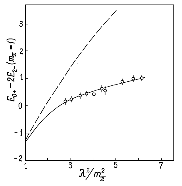
Figure 1:

Figure 2:

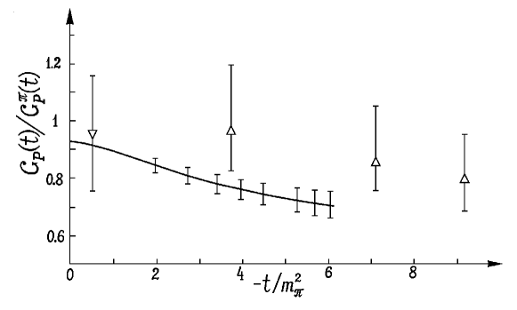
Figure 3:

References

- [1] D.A.Geffen. – Phys. Rev. 125 (1962) 1745. J.Loubaton, J.Tran Thanh Van. – Nucl. Phys. B2 (1967) 342.
- [2] Yu.S.Surovtsev, F.G.Tkebuchava. – JINR Communication P2-4561, Dubna, 1969. T.D.Blokhintseva, Yu.S.Surovtsev, F.G.Tkebuchava. – Yad. Fiz. 21 (1975) 850.
- [3] A.M.Baldin, V.A.Suleymanov. – Phys. Lett. B37 (1971) 305; JINR Communication P2-7096. Dubna, 1973. Yu.S.Surovtsev, F.G.Tkebuchava. – Yad. Fiz. 55 (1992) 2138.
- [4] Yu.S.Surovtsev, F.G.Tkebuchava. – Yad. Fiz. 16 (1972) 1204.
- [5] Yu.V.Kulish. – Yad. Fiz. 16 (1972) 1102. G.Furlan, N.Paver, G.Verzegnassi. – Nuovo Cim. A32 (1976) 75. N.Dombey, B.S.Read. – J. Phys. G: Nucl. Phys. 3 (1977) 1659.
- [6] F.G.Tkebuchava – Nuovo Cim. A47 1978 415.
- [7] G.I.Smirnov, N.M.Shumeyko. – Yad. Fiz. 17 (1973) 1266. A.Bietti, S.Petrarca. – Nuovo Cim. A22 (1974) 595; Lett. Nuovo Cim. 13 (1975) 539.
- [8] Yu.S.Surovtsev, F.G.Tkebuchava. – Yad.Fiz. 21 (1975) 753.
- [9] N.P.Samios. – Phys. Rev. 121 (1961) 275. H.Kobrak. – Nuovo Cim. 20 (1961) 1115. S.Devons et al. – Phys. Rev. 184 (1969) 1356. M.N.Khachaturyan et al. – Phys. Lett. B24 (1967) 349. C.M.Hoffman et al. – Phys. Rev. D28 (1983) 660. H.Fonvieille et al. – Phys. Lett. B233 (1989) 60, 65.
- [10] Yu.K.Akimov et al. – Yad. Fiz. 13 (1971) 748. S.F.Berezhnev et al. –Yad. Fiz. 16 (1972) 185; 18 (1973) 102; 24 (1976) 1127; 26 (1977) 547. G.D.Alekseev et al. – Yad. Fiz. 36 (1982) 322. V.V.Alizade et al. – Yad. Fiz. 33 (1981) 357; 46 (1987) 1360.
- [11] V.M.Baturin et al. – Yad. Fiz. 47 (1988) 708.
- [12] G.Bardin. – Phys. Lett. B255 (1991) 149; B257 (1991) 514.
- [13] R.C.E.Devenish et al. – Phys. Lett. B52 (1974) 227. R.C.E.Devenish et al. – Nuovo Cim. A1 (1971) 475.
- [14] S.A.Goghilidze, Yu.S.Surovtsev, F.G.Tkebuchava. – Yad. Fiz. 45 (1987) 1085.
- [15] S.L.Adler – Ann. Phys. 50 (1968) 189.
- [16] Yu.S.Surovtsev – Author’s summary, 2-11047, Dubna, 1977.
- [17] G.Höhler, E.Pietarinen – Nucl. Phys. B95 (1975) 210.
- [18] G.V.Avakov et al. – Yad. Fiz. 44 (1986) 1471.
- [19] S.Dubnićka et al. – Nuovo Cim. A106 (1993) 1253.
- [20] M.K.Volkov, C.Weiss – JINR Communication E2-96-131, Dubna, 1996.
- [21] Yu.L.Kalinovsky, C.Weiss – Z. Phys. C63 (1994) 275. I.V.Amirkhanov et al. – “Modelling” 6 (1994) 57.
- [22] G.Bardin et al. – Nucl. Phys. A352 (1981) 365; Phys. Lett. B104 (1981) 320.
- [23] V.Brudanin et al. – Nucl. Phys. A587 (1995) 577.
- [24] S.Choi et al. – Phys. Rev. Lett. 71 (1993) 3927.
- [25] Sh.Ishida et al. – Progr. Theor. Phys. 95 (1996) 745; hep-ph/9610359 v2 (27 May 1997). M.Svec – Phys. Rev. D53 (1996) 2343.
- [26] Yu.I.Ivanshin et al. – Nuovo Cim. A107 (1994) 2855.
- [27] Yu.I.Ivanshin, N.B.Skachkov – Nuovo Cim. A108 (1995) 1263.
- [28] A.N. Ivanov, M. Nagy and N.I. Troitskaya: hep-ph/9805347.
- [29] S.B.Gerasimov – Chinese J. Phys. 34 (1996) 848.
- [30] V.A.Meshcheryakov, G.V.Meshcheryakov – Yad. Fiz. 60 (1997) 1400.
- [31] D.Krupa, V.A.Meshcheryakov, Yu.S.Surovtsev – Nuovo Cim. 109 A (1996) 281.