DESY 98-191
hep-ph/9812205
December 1998
THE STATIC POTENTIAL IN QCD
TO TWO LOOPS

Abstract

We evaluate the static QCD potential to two–loop order. Compared to a previous calculation a sizable reduction of the two–loop coefficient $a_{2}$ is found.

1 Introduction

The static potential of (massless) QCD has recently been calculated to two loops [1]. Being a fundamental quantity, it is of importance in many areas, such as NRQCD, quarkonia, quark mass definitions and quark production at threshold. While the one–loop contribution and the two–loop pole terms have been known for a long time [2, 3, 4], the two–loop constant $a_{2}$ (cf. Eqs. (6)-(10)) was found only recently [1]. The fermionic parts of this coefficient were confirmed numerically in [5], taking the $m_{q}\!\rightarrow\!0$ limit of a calculation involving massive fermion loops. The aim of this work is to evaluate $a_{2}$ analytically, using an independent method.

The static potential is defined in a manifestly gauge invariant way via the vacuum expectation value of a Wilson loop [4, 6],

$$V(r)=-\lim_{T\rightarrow\infty}\frac{1}{T}\,\ln\left\langle\vphantom{A^{b}_{\mu}}{\rm tr}{\cal P}\exp\left(ig\oint_{\Gamma}dx_{\mu}A_{\mu}\right)\right\rangle\;.$$ (1)

Here, $\Gamma$ is taken as a rectangular loop with time extension $T$ and spatial extension $r$, and $A_{\mu}$ is the vector potential in the fundamental representation.

In a perturbative analysis it can be shown that, at least to the order needed here, all contributions to Eq. (1) containing connections to the spatial components of the gauge fields $A_{i}(\mbox{\boldmath$r$},\pm T/2)$ vanish in the limit of large time extension $T$. Hence, the definition can be reduced to

$$V_{\rm pert}(r)=-\lim_{T\rightarrow\infty}\frac{1}{T}\,\ln\left\langle\vphantom{A^{b}_{\mu}}{\rm tr}{\cal T}\exp\left(-\int_{x}J_{\mu}^{a}A_{\mu}^{a}\right)\right\rangle\;,$$ (2)

where ${\cal T}$ means time ordering and the static sources separated by the distance $r=|\mbox{\boldmath$r$}-\mbox{\boldmath$r$}\,^{\prime}|$ are given by

$$J_{\mu}^{a}(x)=ig\,\delta_{\mu 0}T^{a}\,\left[\,\delta(\mbox{\boldmath$x$}-\mbox{\boldmath$r$})-\delta(\mbox{\boldmath$x$}-\mbox{\boldmath$r$}\,^{\prime})\,\right]\,\;,$$ (3)

where $T^{a}$ are the generators in the fundamental representation. In the case of QCD the gauge group is $SU(3)$. The calculation will be carried out for an arbitrary compact semi-simple Lie group with structure constants defined by the Lie algebra $[T^{a},T^{b}]=if^{abc}T^{c}$. The Casimir operators of the fundamental and adjoint representation are $T^{a}T^{a}=C_{F}$ and $f^{acd}f^{bcd}=C_{A}\delta^{ab}$. $tr(T^{a}T^{b})=T_{F}\delta^{ab}$ is the trace normalization, while $n_{f}$ denotes the number of massless quarks.

Expanding the expression in Eq. (2) perturbatively, one encounters in addition to the usual Feynman rules the source–gluon vertex $ig\delta_{\mu 0}T^{a}$, with an additional minus sign for the antisource. Furthermore, the time–ordering prescription generates step functions, which can be viewed as source propagators, analogous to the heavy–quark effective theory (HQET) [7].

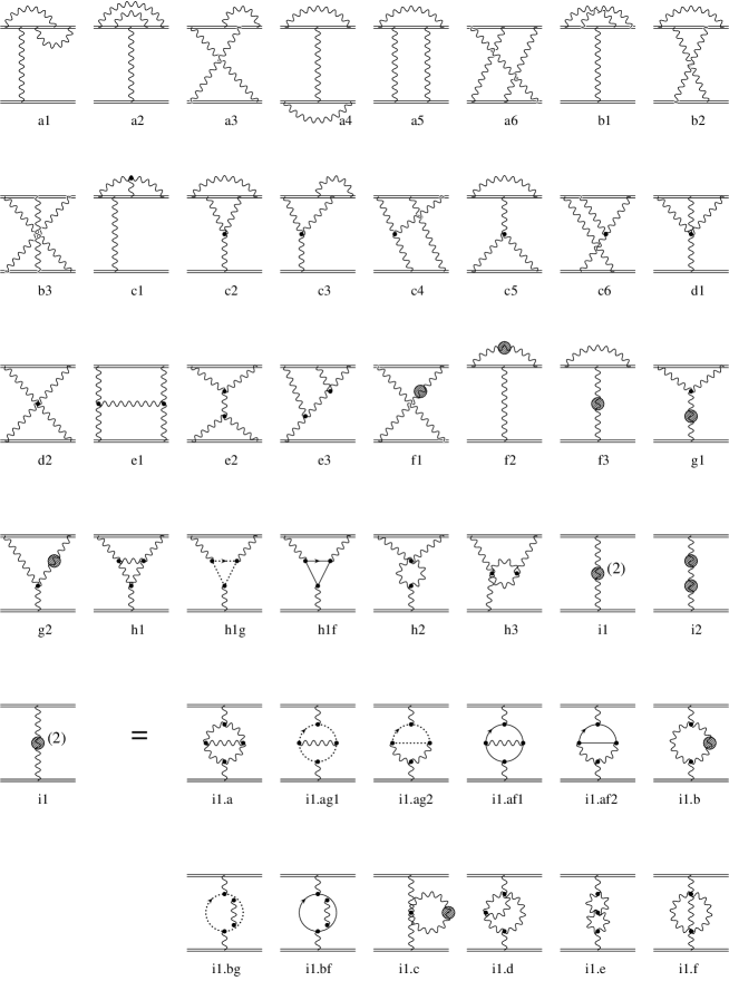
Figure 1: Classes of two–loop diagrams contributing to the static potential. Double, wiggly, dotted and solid lines denote source, gluon, ghost and (light) fermion propagators, respectively. A blob on a gluon line stands for one–loop self–energy corrections.

Concerning the generation of the complete set of Feynman diagrams contributing to the two–loop static potential, there are some subtleties connected with the logarithm in the definition (2). All this is explained in detail in [1, 3], so we only list the relevant diagrams here (see Fig.1). Note that the aforementioned papers are based on the Feynman gauge, while we use general covariant gauges, resulting in an enlarged set of diagrams.

2 Method

The method employed in this work can be briefly summarized as follows:

$\bullet$ All dimensionally regularized (tensor-) integrals are reduced to pure propagator integrals by a generalization of Tarasov’s method [8]. The resulting expressions are then mapped to a minimal set of five scalar integrals by means of recurrence relations, again generalizing [8] as well as [9] to the case including static (noncovariant) propagators. These two steps are implemented into a FORM [11] package. Thus, we constructed our method to be complementary to the calculation in [1], assuring a truly independent check. At this stage, one obtains analytic coefficient functions (depending on the generic space–time dimension $D$ as well as on the color factors and the bare coupling), multiplying each of the basic integrals.

$\bullet$ The basic scalar integrals are then solved analytically. Expanding the result around $D=4$ (which is done in both MAPLE [12] and Mathematica [13] considering the complexity of the expressions) and renormalizing, one obtains the final result to be compared with [1].

Important checks of the calculation are the comparison of the pole terms of individual gluonic diagrams given in [3], the gauge independence of appropriate classes of diagrams, the confirmation of cancellation of infrared divergencies, and the correct renormalization properties.

3 Renormalization and result

The renormalized quantities in $D=4-\epsilon$ dimensions are conventionally defined by

$$V\equiv\mu^{\epsilon}V_{R}\quad,\quad\frac{g^{2}}{16\pi^{2}}\equiv Z\mu^{\epsilon}a_{R}\;,$$ (4)

where the subscript $R$ denotes the renormalized quantities. The factor $Z$ is assumed to have an expansion in the renormalized coupling, $Z=1+a_{R}Z^{{}^{\prime}}(\epsilon)+a_{R}^{2}Z^{{}^{\prime\prime}}(\epsilon)+...$, and we choose to work in the ${\overline{{\rm MS}}}$ scheme, related to the MS scheme by the scale redefinition $\mu^{2}=\bar{\mu}^{2}e^{\gamma}/4\pi$ .

The needed counterterms read explicitly

$$Z^{{}^{\prime}}_{{{}\over{\rm MS}}}=-\frac{2}{\epsilon}\,\beta_{0}\quad,\quad Z^{{}^{\prime\prime}}_{{{}\over{\rm MS}}}=\frac{4}{\epsilon^{2}}\,\beta_{0}^{2}-\frac{1}{\epsilon}\,\beta_{1}\;.$$ (5)

Here, the coefficients of the Beta function are defined by the running coupling, $\mu^{2}\partial_{\mu^{2}}\,a_{R}=-\beta_{0}a_{R}^{2}-\beta_{1}a_{R}^{3}-...$, $\beta_{0}=\frac{11}{3}\,C_{A}-\frac{4}{3}\,T_{F}n_{f}$ and $\beta_{1}=\frac{34}{3}\,C_{A}^{2}-4C_{F}T_{F}n_{f}-\frac{20}{3}\,C_{A}T_{F}n_{f}$. The results of our calculation yield indeed Eq. (5).

As a further check on the pole terms, the vertex and gluon wave function renormalization constants ($Z_{1}$ and $Z_{3}^{-1}$, respectively) have been extracted separately from the diagrams. They depend on the gauge parameter $\xi$ and agree with the ones given in [14].

The renormalized potential now reads $V_{\rm pert}(r)=\int\!\frac{d^{3}q}{(2\pi)^{3}}\,\exp(i\mbox{\boldmath$q$}\mbox{\boldmath$r$})V(\mbox{\boldmath$q$}^{2})\,$, with

$$V(\mbox{\boldmath$q$}^{2}) = -\frac{C_{F}16\pi^{2}}{\mbox{\boldmath$q$}^{2}}\,a_{{}\over{\rm MS}}\left\{1+a_{{}\over{\rm MS}}\,c_{1\,{{}\over{\rm MS}}}\left(\frac{\bar{\mu}^{2}}{\mbox{\boldmath$q$}^{2}}\right)+a_{{}\over{\rm MS}}^{2}\,c_{2\,{{}\over{\rm MS}}}\left(\frac{\bar{\mu}^{2}}{\mbox{\boldmath$q$}^{2}}\right)+...\right\}$$ (6)

where

$$c_{1\,{{}\over{\rm MS}}}(x) = a_{1}+\beta_{0}\ln(x)\;,$$ (7)

$$c_{2\,{{}\over{\rm MS}}}(x) = a_{2}+\beta_{0}^{2}\ln^{2}(x)+(\beta_{1}+2\beta_{0}a_{1})\ln(x)$$ (8)

and

$$a_{1} = \frac{31}{9}\,C_{A}-\frac{20}{9}\,T_{F}n_{f}\;,$$ (9)

$$a_{2} = \left(\frac{4343}{162}+4\pi^{2}-\frac{\pi^{4}}{4}+\frac{22}{3}\zeta(3)\right)C_{A}^{2}-\left(\frac{1798}{81}+\frac{56}{3}\,\zeta(3)\right)C_{A}T_{F}n_{f}$$ (10)

$$-\left(\frac{55}{3}-16\zeta(3)\right)C_{F}T_{F}n_{f}+\frac{400}{81}\,T_{F}^{2}n_{f}^{2}\;.$$

As it has to be, the coefficients prove to be gauge independent. Comparing our two-loop result for $a_{2}$ with [1], we find a discrepancy of $2\pi^{2}$ in the pure Yang–Mills term ($\propto C_{A}^{2}$). This amounts to a $30\%$ decrease of $a_{2}$ for the case of $n_{f}=0$, and a $50\%$ decrease for $n_{f}=5$ (for $SU(3)$), which is the case needed for $t\bar{t}$ threshold investigations. This difference can be traced back to a specific set of diagrams, as outlined below.

The origin of the discrepancy is Eq. (14) in the second paper of [1]. To explain the crucial point, let us introduce some notations first: We have two types of denominators, $D_{i}\equiv D(k_{i})=\frac{1}{k_{i}^{2}}\,$, stemming from gluon, ghost and fermion propagators, and $S_{i}\equiv S(k_{i})=\frac{1}{v\cdot k_{i}+i\varepsilon}\,$, with $v=(1,\mbox{\boldmath$0$})$, stemming from the source propagators. The loop momenta are $k_{1}$, $k_{2}$, $k_{3}=k_{1}-q$, $k_{4}=k_{2}-q$, $k_{5}=k_{1}-k_{2}$, where $q=(0,\mbox{\boldmath$q$})$ is the external momentum. We abbreviate the integration measure as $\int_{i}\equiv\mu^{\epsilon}\int\!\frac{d^{D}k_{i}}{(2\pi)^{D}}\,$, while products of propagators will be written like $D_{1}D_{2}\equiv D_{12}$ etc.

Adding the diagrams in question gives (neglecting the color factors)

$$\;\parbox{22.76219pt}{ \begin{picture}(8.0,6.0)\put(0.0,0.0){\line(1,0){8.0}} \put(0.0,6.0){\line(1,0){8.0}} \put(0.0,0.0){\line(5,6){5.0}} \put(3.0,0.0){\line(5,6){5.0}} \put(0.0,6.0){\line(4,-3){8.0}} \end{picture}}\;+\;\parbox{22.76219pt}{ \begin{picture}(8.0,6.0)\put(0.0,0.0){\line(1,0){8.0}} \put(0.0,6.0){\line(1,0){8.0}} \put(0.0,6.0){\line(5,-6){5.0}} \put(3.0,6.0){\line(5,-6){5.0}} \put(0.0,0.0){\line(4,3){8.0}} \end{picture}}\;+\;\parbox{22.76219pt}{ \begin{picture}(8.0,6.0)\put(0.0,0.0){\line(1,0){8.0}} \put(0.0,6.0){\line(1,0){8.0}} \put(4.0,0.0){\line(0,1){6.0}} \put(0.0,0.0){\line(4,3){8.0}} \put(0.0,6.0){\line(4,-3){8.0}} \end{picture}}\; = \int_{1}\int_{2}\left(D_{235}S_{1125}+D_{145}S_{1125}+D_{235}S_{1122}\right)$$ (11)

$$= \int_{1}\int_{2}\left(D_{145}S_{1125}+D_{235}S_{1225}\right)$$

$$= \int_{1}\int_{2}D_{145}S_{112}\left(S_{5}+S_{\bar{5}}\right)\;,$$

where the identity $S_{1}S_{2}=S_{5}(S_{2}-S_{1})$ (compare [1], §4) was used for the last term of the first line, and the trivial exchange of loop variables $k_{1}\leftrightarrow k_{2}$ was done in the last term of line two. In the last line, $S_{\bar{5}}=S(-k_{5})$. One then obtains

$$S_{5}+S_{\bar{5}} = \frac{1}{(k_{10}-k_{20})+i\varepsilon}+\frac{1}{-(k_{10}-k_{20})+i\varepsilon}$$ (12)

$$= -\frac{2i\varepsilon}{(k_{10}-k_{20})^{2}+\varepsilon^{2}}\quad\stackrel{{\scriptstyle\varepsilon\rightarrow 0^{+}}}{{\longrightarrow}}\quad-2\pi i\delta\left(k_{10}-k_{20}\right)\;.$$

Hence, contrary to the assumption in [1], the sum of the integrands in Eq. (11) reduces to a delta distribution multiplying the remaining propagators.

Now, considering the color traces as well as the gluon-source couplings, one gets as a contribution to the bare static potential (for simplicity, we use the Feynman gauge here to make the point clear)

$${\rm diag.a6+diag.b3} = -\frac{g^{6}}{4}\,C_{F}C_{A}^{2}\left(\;\parbox{22.76219pt}{ \begin{picture}(8.0,6.0)\put(0.0,0.0){\line(1,0){8.0}} \put(0.0,6.0){\line(1,0){8.0}} \put(0.0,0.0){\line(5,6){5.0}} \put(3.0,0.0){\line(5,6){5.0}} \put(0.0,6.0){\line(4,-3){8.0}} \end{picture}}\;+\;\parbox{22.76219pt}{ \begin{picture}(8.0,6.0)\put(0.0,0.0){\line(1,0){8.0}} \put(0.0,6.0){\line(1,0){8.0}} \put(0.0,6.0){\line(5,-6){5.0}} \put(3.0,6.0){\line(5,-6){5.0}} \put(0.0,0.0){\line(4,3){8.0}} \end{picture}}\;\right)-\frac{g^{6}}{2}\,C_{F}C_{A}^{2}\;\parbox{22.76219pt}{ \begin{picture}(8.0,6.0)\put(0.0,0.0){\line(1,0){8.0}} \put(0.0,6.0){\line(1,0){8.0}} \put(4.0,0.0){\line(0,1){6.0}} \put(0.0,0.0){\line(4,3){8.0}} \put(0.0,6.0){\line(4,-3){8.0}} \end{picture}}\;$$

$$= -\frac{g^{6}}{4}\,C_{F}C_{A}^{2}\;\parbox{22.76219pt}{ \begin{picture}(8.0,6.0)\put(0.0,0.0){\line(1,0){8.0}} \put(0.0,6.0){\line(1,0){8.0}} \put(4.0,0.0){\line(0,1){6.0}} \put(0.0,0.0){\line(4,3){8.0}} \put(0.0,6.0){\line(4,-3){8.0}} \end{picture}}\;-\frac{g^{6}}{4}\,C_{F}C_{A}^{2}\left(\;\parbox{22.76219pt}{ \begin{picture}(8.0,6.0)\put(0.0,0.0){\line(1,0){8.0}} \put(0.0,6.0){\line(1,0){8.0}} \put(0.0,0.0){\line(5,6){5.0}} \put(3.0,0.0){\line(5,6){5.0}} \put(0.0,6.0){\line(4,-3){8.0}} \end{picture}}\;+\;\parbox{22.76219pt}{ \begin{picture}(8.0,6.0)\put(0.0,0.0){\line(1,0){8.0}} \put(0.0,6.0){\line(1,0){8.0}} \put(0.0,6.0){\line(5,-6){5.0}} \put(3.0,6.0){\line(5,-6){5.0}} \put(0.0,0.0){\line(4,3){8.0}} \end{picture}}\;+\;\parbox{22.76219pt}{ \begin{picture}(8.0,6.0)\put(0.0,0.0){\line(1,0){8.0}} \put(0.0,6.0){\line(1,0){8.0}} \put(4.0,0.0){\line(0,1){6.0}} \put(0.0,0.0){\line(4,3){8.0}} \put(0.0,6.0){\line(4,-3){8.0}} \end{picture}}\;\right)\;.$$

While in [1] the latter term was discarded, we evaluate it in $D=4-\epsilon$ dimensions to give

$$\;\parbox{22.76219pt}{ \begin{picture}(8.0,6.0)\put(0.0,0.0){\line(1,0){8.0}} \put(0.0,6.0){\line(1,0){8.0}} \put(0.0,0.0){\line(5,6){5.0}} \put(3.0,0.0){\line(5,6){5.0}} \put(0.0,6.0){\line(4,-3){8.0}} \end{picture}}\;+\;\parbox{22.76219pt}{ \begin{picture}(8.0,6.0)\put(0.0,0.0){\line(1,0){8.0}} \put(0.0,6.0){\line(1,0){8.0}} \put(0.0,6.0){\line(5,-6){5.0}} \put(3.0,6.0){\line(5,-6){5.0}} \put(0.0,0.0){\line(4,3){8.0}} \end{picture}}\;+\;\parbox{22.76219pt}{ \begin{picture}(8.0,6.0)\put(0.0,0.0){\line(1,0){8.0}} \put(0.0,6.0){\line(1,0){8.0}} \put(4.0,0.0){\line(0,1){6.0}} \put(0.0,0.0){\line(4,3){8.0}} \put(0.0,6.0){\line(4,-3){8.0}} \end{picture}}\; = \frac{6(D-4)(3D-11)}{(D-5)}\,\frac{1}{\mbox{\boldmath$q$}^{2}}\int_{1}\int_{2}D_{235}S_{12}$$ (13)

$$= -\frac{1}{32\pi^{2}}\,\frac{1}{\mbox{\boldmath$q$}^{2}}+O(\epsilon)\;.$$

Note that the factor of $(D-4)$ in the numerator cancels the single pole in the scalar integral, such that only the constant part of $a_{2}$ is affected by this discussion, while the pole terms are not changed by the omission of this term. Hence, dividing out the overall factor $\left(-\frac{C_{F}g^{6}}{(16\pi^{2})^{2}\mbox{\boldmath$q$}^{2}}\right)$, we identify the $2\pi^{2}C_{A}^{2}$ difference with respect to [1] .

The static potential can be used for a definition of an effective charge, which is conventionally called $a_{\scriptscriptstyle V}$. Defining $V(\mbox{\boldmath$q$}^{2})=-C_{F}16\pi^{2}a_{\scriptscriptstyle V}/\mbox{\boldmath$q$}^{2}$, one can use the knowledge of the three–loop coefficient $\beta_{2}^{{}\over{\rm MS}}$ [14] to derive the corresponding coefficient in the $V$–scheme from Eq. (6). While $\beta_{0}$ and $\beta_{1}$ are universal, one finds

$$\beta_{2}^{\scriptscriptstyle V} = \beta_{2}^{{}\over{\rm MS}}-a_{1}\beta_{1}+(a_{2}-a_{1}^{2})\beta_{0}$$ (15)

$$= \left(\frac{206}{3}+\frac{44\pi^{2}}{3}-\frac{11\pi^{4}}{12}+\frac{242}{9}\,\zeta(3)\right)C_{A}^{3}$$

$$-\left(\frac{445}{9}+\frac{16\pi^{2}}{3}-\frac{\pi^{4}}{3}+\frac{704}{9}\,\zeta(3)\right)C_{A}^{2}T_{F}n_{f}+\left(\frac{2}{9}+\frac{224}{9}\,\zeta(3)\right)C_{A}T_{F}^{2}n_{f}^{2}$$

$$-\left(\frac{686}{9}-\frac{176}{3}\,\zeta(3)\right)C_{A}C_{F}T_{F}n_{f}+2C_{F}^{2}T_{F}n_{f}+\left(\frac{184}{9}-\frac{64}{3}\,\zeta(3)\right)C_{F}T_{F}^{2}n_{f}^{2}\;.$$

The new value for $a_{2}$ leads, for $SU(3)$ and $n_{f}=5$, to a 50% decrease of $\beta_{2}^{\scriptscriptstyle V}$ compared to the formula given in [1].

Summarizing, we have re-calculated the two–loop static potential by a method complementary to the approach in [1]. We have developed an algorithm which enables us to work in general covariant gauges throughout. Confirming the fermionic contributions to the two–loop coefficient $a_{2}$, we find a substantial deviation in the pure gluonic part of $a_{2}$. The source of the discrepancy could be identified.

We would like to thank W. Buchmüller, M. Spira, T. Teubner and M. Peter for valuable discussions and correspondence, respectively.

References

[1] M. Peter, Phys. Rev. Lett. 78 (1997) 602, hep-ph/9610209;
Nucl. Phys. B 501 (1997) 471, hep-ph/9702245.
[2] L. Susskind, Coarse grained quantum chromodynamics
in R. Balian and C.H. Llewellyn Smith (eds.),
Weak and electromagnetic interactions at high energy
(North Holland, Amsterdam, 1977).
[3] W. Fischler, Nucl. Phys. B 129 (1977) 157.
[4] A. Billoire, Phys. Lett. B 92 (1980) 343.
[5] M. Melles, Phys. Rev. D 58 (1998) 114004, hep-ph/9805216.
[6] E. Eichten and F. Feinberg, Phys. Rev. D 23 (1981) 2724.
[7] E. Eichten and B. Hill, Phys. Lett. B 234 (1990) 511;
for a review and references, see M. Neubert, Phys. Rep. 245C (1994) 259,
hep-ph/9306320.
[8] O.V. Tarasov, Nucl. Phys. B 502 (1997) 455, hep-ph/9703319.
[9] K.G. Chetyrkin and F.V. Tkachov, Nucl. Phys. B 192 (1981) 159.
[10] Y. Schröder, in preparation.
[11] J.A.M. Vermaseren, Symbolic Manipulation
with FORM (CAN, Amsterdam, 1991).
[12] B.W. Char, K.O. Geddes, G.H. Gonnet, B.L. Leong,
M.B. Monagan, S.M. Watt, Maple V, (Springer, New York, 1991).
[13] S. Wolfram, Mathematica – A System for
Doing Mathematics by Computer, (Addison-Wesley, Redwood City,
CA, 1988).
[14] see, e.g., S.A. Larin and J.A.M. Vermaseren,
Phys. Lett. B 303 (1993) 334, hep-ph/9302208.