The Supersymmetric QCD Radiative Corrections to Top Quark Semileptonic Decays

Abstract

The one-loop supersymmetric QCD corrections to the top quark semileptonic decays $t\rightarrow b~{}\bar{l}~{}{\nu_{l}}$ are considered. The corrections are found to reduce the decay width. In the still acceptable parameter space the corrections to the percentage change in top quark semileptonic decay width can reach the level of -0.7%.

PACS numbers: 11.30.Pb, 12.38.Bx, 14.65.Ha

Keyword(s): SUSY QCD, RADIATIVE CORRECTIONS, TOP DECAY

I Introduction

The discovery of the top quark in 1995 [1, 2, 3] marked the triumph of the Standard Model(SM) of particle physics. Since the discovery, more interest on top quark physics research is stimulated in both experimental and theoretical respects. Because of its large mass which is close to the electroweak scale, the top quark physics research may play an important role in the study of the electroweak symmetry breaking and therefore of the origin of the fermion masses. Through the study on it people also hope to find clues of possible ”new physics”.

Within the framework of SM the dominant top quark decay channel is $t\rightarrow bW$, which has a time scale $\tau_{W}$ much shorter than the time scale of the non-perturbative QCD effect. This character of top quark makes it behaves almost like a free particle, which is helpful in the precise study on it. With the operation of CERN Large Hadron Collider (LHC) in the future there will be enormous top quark events obtained in every year and that provides it practically possible to make the more detailed study on many properties of top quark.

Because of the importance of top quark decay stated above, a lot theoretical efforts have been made in the studies of radiative corrections to its decays. In the SM, the QCD and electroweak corrections to the $t\rightarrow bW$ decay can be found in [4, 5]. Recently, the order ${\cal O}(\alpha_{s}^{2})$ QCD radiative corrections on some specific situations are presented in literatures [6, 7, 8]. Beyond the SM, based on the two Higgs doublet model (2HDM) the radiative corrections to $t\rightarrow bW$ are calculated in [9]. The supersymmetric (SUSY) contributions of both QCD and electroweak are given in [10].

The top quark semileptonic decays is also one of the major and important decay channels of the top quark, because there is a great portion of W decay probability will proceed leptonic pattern. Before the top quark was detected, it was long believed that the top mass maybe less than that of W boson’s. So, the $t\rightarrow b~{}\bar{l}~{}{\nu_{l}}$ processes [11] were taken into consideration even earlier than $t\rightarrow bW$ process. And also the QCD corrections to it was completed [12, 13], which was found coincides with results in Ref.[4] after taking the $W$ on its mass shell. In this paper we present a calculation on SUSY QCD radiative corrections to the top quark semileptonic decays, which we find is still not appeared in literatures.

II Formalism

The relevant Feynman diagrams for the one-loop virtual gluino corrections to the top quark semileptonic decay process $t(p)\rightarrow b(k_{1})\bar{l}(k_{2})v_{l}(k_{3})$ are shown in Fig. 1. The tree-level amplitude (Fig.1(a)) can be written down straightforwardly using the standard Feynman rules,

$$M_{0}(t\rightarrow b~{}\bar{l}~{}{\nu_{l}})={2\pi\alpha\over x_{W}(k^{2}-M_{W}^{2}+i\Gamma_{W}M_{W})}[\bar{u}_{b}(k_{1})\gamma_{\mu}P_{L}u_{t}(p)][\bar{u}_{\nu_{l}}(k_{3})\gamma^{\mu}P_{L}v_{\bar{l}}(k_{2})].$$ (1)

Here, $k=k_{2}+k_{3}$ is the momentum transfer carried by the W boson, $P_{L}$ is the left-handed helicity projection operators, and the $x_{W}$ is the square of the sine of the Weinberg angle, $x_{W}={\rm sin}^{2}\theta_{W}$.

In one-loop calculations, we will use dimensional regularization to control all the ultraviolet divergences in the virtual loop corrections and we will adopt the on-mass-shell renormalization scheme [14, 15]. It is noted that dimensional reduction approach is widely used in the calculations of the radiative corrections in the minimal supersymmetric standard model (MSSM) as it automatically preserves the supersymmetry (at least to one-loop order), while dimensional regularization does not. But in the calculations of SUSY QCD corrections to the process concerned, the dimensional reduction scheme is the same with the conventional dimensional regularization one. The one-loop amplitude of the discussed process can be written as

$$\delta M=M^{con}+M^{unr},$$ (2)

where $M^{con}$ and $M^{unr}$ represent the counterterm and the un-renormalized amplitude, respectively. And,

$$M^{con} = {1\over 2}(Z_{Lt}+Z_{Lb})M_{0},$$ (3)

where

$$Z_{Lt} = {\alpha_{s}\over 4\pi m_{t}^{2}}\{\cos^{2}\theta[(m_{\tilde{t}_{2}}^{2}-m_{\tilde{g}}^{2})(B_{0}(2)-B_{0}(4))-m_{t}^{2}B_{0}(3)$$ (7)

$$+(m_{t}^{2}(-m_{\tilde{g}}^{2}+m_{\tilde{t}_{2}}^{2}-m_{t}^{2})(\dot{B}_{0}(3)+\dot{B}_{0}(4))]+4m_{\tilde{g}}m_{t}^{3}\cos\theta\sin\theta(\dot{B}_{0}(3)+\dot{B}_{0}(4))$$

$$+\sin^{2}\theta[(m_{\tilde{t}_{1}}^{2}-m_{\tilde{g}}^{2})(B_{0}(1)-B_{0}(3))-m_{t}^{2}B_{0}(4)$$

$$+(m_{t}^{2}(-m_{\tilde{g}}^{2}+m_{\tilde{t}_{1}}^{2}-m_{t}^{2})(\dot{B}_{0}(3)+\dot{B}_{0}(4))]\}$$

and

$$Z_{Lb} = Z_{Lt}[\tilde{t}\rightarrow\tilde{b},\theta\rightarrow 0]$$ (8)

are the wave-function renormalization constants for top and bottom quark respectively. In above and following equations the $B_{0}$, $C_{0}$, $C_{i}$, and $C_{i,j}$ functions result from the evaluation of certain loop integrals, expressions for which can be found in [14, 16]. In equation (4), $\dot{B}_{0}(p^{2},m_{a}^{2},m_{b}^{2})=\partial B_{0}(p^{2},m_{a}^{2},m_{b}^{2})/\partial p^{2}$, and $(1)-(4)$ are abbreviations of variables in $B_{0}$ function, which represent $(0,m_{\tilde{g}}^{2},m_{\tilde{t}_{1}}^{2})$, $(0,m_{\tilde{g}}^{2},m_{\tilde{t}_{2}}^{2})$, $(m_{t}^{2},m_{\tilde{g}}^{2},m_{\tilde{t}_{1}}^{2})$ and $(m_{t}^{2},m_{\tilde{g}}^{2},m_{\tilde{t}_{2}}^{2})$, respectively. Throughout our calculations, we will omit the bottom scalar left- and right-handed mixing, but consider the top scalar mixing, because of the small bottom quark mass compared with the top quark mass, the definition of the mixing angle of top scalar $\theta$ can be found in next section.

$$M^{unr} = {\alpha_{s}\alpha\over x_{W}(k^{2}-M_{W}^{2}+i\Gamma_{W}M_{W})}\bar{u}_{b}(k_{1})(f_{1}\gamma_{\mu}P_{L}+f_{2}k_{1\mu}P_{R}+f_{3}k_{1\mu}P_{L}+f_{4}\hbox to0.0pt{/\hss}kk_{1\mu}P_{L}+f_{5}p_{\mu}P_{R}$$ (9)

$$+ f_{6}p_{\mu}P_{L}+f_{7}\hbox to0.0pt{/\hss}kp_{\mu}P_{L}+f_{8}k_{\mu}P_{R}+f_{9}k{\mu}P_{L}+f_{10}\hbox to0.0pt{/\hss}kk_{\mu}P_{L})u_{t}(p)\bar{u}_{v_{l}}(k_{3})\gamma_{\mu}P_{L}v_{\bar{l}}(k_{2}),$$ (10)

where

$$f_{1} = 2(\cos^{2}\theta C_{00}(1)+\sin^{2}\theta C_{00}(2)),$$ (11)

$$f_{2} = \sin\theta\cos\theta(C_{0}(2)-C_{0}(1)+2C_{1}(2)-2C_{1}(1)),$$ (12)

$$f_{3} = m_{b}(\cos^{2}\theta(C_{0}(1)+3C_{1}(1)+2C_{11}(1))+\sin^{2}\theta(C_{0}(2)+3C_{1}(2)+2C_{11}(2))),$$ (13)

$$f_{4} = -\cos^{2}\theta(C_{2}(1)+2C_{12}(1))-\sin^{2}\theta(C_{2}(2)+2C_{12}(2)),$$ (14)

$$f_{5} = \sin\theta\cos\theta m_{\tilde{g}}(C_{0}(1)-C_{0}(2)),$$ (15)

$$f_{6} = -\cos^{2}\theta(C_{0}(1)+C_{1}(1))-\sin^{2}\theta(C_{0}(2)+C_{1}(2)),$$ (16)

$$f_{7} = \cos^{2}\theta C_{2}(1)+\sin^{2}\theta C_{2}(2),$$ (17)

$$f_{8} = \sin(2\theta)m_{\tilde{g}}(C_{2}(1)-C_{2}(2)),$$ (18)

$$f_{9} = -2(\cos^{2}\theta(C_{2}(1)+C_{12}(1))+\sin^{2}\theta(C_{2}(2)+C_{12}(2))),$$ (19)

$$f_{10} = 2(\cos^{2}\theta C_{22}(1)+\sin^{2}\theta C_{22}(2)).$$ (20)

Here, (1) and (2) in the parentheses of above equations are the variables of $C$ function which represent $(m_{b}^{2},m_{t}^{2},k^{2},m_{\tilde{b}_{1}}^{2}m_{\tilde{g}}^{2},m_{\tilde{t}_{1}}^{2})$ and $(m_{b}^{2},m_{t}^{2},k^{2},m_{\tilde{b}_{1}}^{2}m_{\tilde{g}}^{2},m_{\tilde{t}_{2}}^{2})$ for simplicity, respectively.

The corresponding amplitude squared of the process $t\rightarrow b~{}\bar{l}~{}v_{l}$ can then be expressed as

$$\overline{{\sum}}\left|M\right|^{2}=\overline{{\sum}}\left|M_{0}\right|^{2}+2Re(\overline{{\sum}}\delta MM_{0}^{\dagger}),$$ (21)

III Results and Discussion

In our numerical calculations, we choose $\alpha_{s}=0.118$, $\alpha=1/128$, $M_{Z}=91.187$ GeV, $M_{W}=80.33$ GeV, $\Gamma_{W}=2.1$ GeV, $m_{t}=176.0$ GeV, and $m_{b}=4.5$ GeV, which are commonly used in literatures [17].

In the MSSM the squark mass eigenstates $\tilde{q}_{1}$ and $\tilde{q}_{2}$ are related to the current eigenstates $\tilde{q}_{L}$ and $\tilde{q}_{R}$ by

$$\left(\begin{array}[]{c}\tilde{q}_{1}\\ \tilde{q}_{2}\end{array}\right)=R^{\tilde{q}}\left(\begin{array}[]{c}\tilde{q}_{L}\\ \tilde{q}_{R}\end{array}\right)$$ (26)

with

$$R^{\tilde{q}}=\left(\begin{array}[]{cc}\cos\theta&\sin\theta\\ -\sin\theta&\cos\theta\end{array}\right).$$ (29)

The mixing angle $\theta$ and the masses $m_{\tilde{q}_{1,2}}$ of squarks can be obtained by diagonalizing the following mass matrices [18]

$$M^{2}_{\tilde{q}}=\left(\begin{array}[]{cc}M_{LL}^{2}&m_{q}M_{LR}\\ m_{q}M_{RL}&M_{RR}^{2}\end{array}\right),$$ (32)

where

$$M_{LL}^{2}=m_{\tilde{Q}}^{2}+m_{q}^{2}+m_{z}^{2}\cos 2\beta(I_{q}^{3L}-e_{q}x_{W}),$$ (33)

$$M_{RR}^{2}=m_{\tilde{U},\tilde{D}}^{2}+m_{q}^{2}+m_{z}^{2}e_{q}x_{W}\cos 2\beta,$$ (34)

$$M_{LR}=M_{RL}=\left\{\begin{array}[]{ll}A_{t}-\mu\cot\beta&(\tilde{q}=\tilde{t}),\\ A_{b}-\mu\tan\beta&(\tilde{q}=\tilde{b}).\end{array}\right.$$ (37)

In Eq.(32)-(37), $m_{\tilde{Q}}^{2}$, $m_{\tilde{U},\tilde{D}}^{2}$ are soft SUSY breaking mass terms of the left- and right-handed squark, respectively; $\mu$ is the coefficient of the $H_{1}H_{2}$ mixing term in the superpotential; $A_{t}$ and $A_{b}$ are the coefficients of the dimension-three trilinear soft SUSY-breaking term; $I_{q}^{3L},e_{q}$ are the weak isospin and electric charge of the squark $\tilde{q}$. From Eqs.(26) and (32) $m_{\tilde{t}_{1,2}}$ and $\theta$ can be derived out

$$m^{2}_{\tilde{t}_{1,2}} = {1\over 2}\left[M^{2}_{LL}+M^{2}_{RR}\mp\sqrt{(M^{2}_{LL}-M^{2}_{RR})^{2}+4m^{2}_{t}M^{2}_{LR}}\right],$$ (38)

$$\tan\theta = {m^{2}_{\tilde{t}_{1}}-M^{2}_{LL}\over m_{t}M_{LR}}.$$ (39)

The results of percentage change in the top quark semileptonic decay width, $\delta\Gamma_{SL}/\Gamma_{SL}$, after considering the SUSY QCD corrections are presented in Figs. 2-4. In numerical calculations we also assume $\mu=-100$ GeV and $m_{\tilde{U}}=m_{\tilde{D}}=m_{\tilde{Q}}=A_{t}=m_{S}$ (the so-called global SUSY). From the Tevatron dileptons and jet +$\not\!\!\!{{E}_{T}}$ analysis under certain assumptions and parameter inputs, people get that $m_{\tilde{g}}>180$ GeV [19] and $m_{\tilde{q}}>90$ GeV (especially for the stop lower limit) presently [20].

In Fig. 2 we show the relative corrections of one-loop SUSY QCD to the $t\rightarrow b~{}\bar{l}~{}{\nu_{l}}$ decay widths as the function of $m_{S}$, while keeping the $m_{\tilde{g}}$ and tan$\beta$ fixed. Taking $m_{\tilde{g}}=200$ GeV and tan$\beta=2$ we find that the total relative correction for $l=e,~{}\mu,~{}\tau$ reaches -0.6% from -0.33% as the $m_{S}$ goes from 100 GeV to 300 GeV. In Fig. 3 we take the $m_{S}$ and tan$\beta$ fixed, $m_{S}=100$ and tan$\beta=2$, and show the relation of relative correction with the $m_{\tilde{g}}$. It can be seen that the relative correction grows up till -0.9% with the decline of $m_{\tilde{g}}$ down to 150 GeV. In Fig.4 we show the dependence of relative correction on tan$\beta$ when take $m_{S}=100$ GeV and $m_{\tilde{g}}=200$ GeV. The correction varies from -0.6% to -0.41% with tan$\beta$ going from 2 to 50, and it is interesting to note that the curve gradually goes to be flat with the growth of tan$\beta$, which indicates that the correction is not closely sensitive to the value of tan$\beta$ as it larger than 10.

In conclusion, we have calculated the SUSY QCD corrections to the semileptonic top quark decays. It is found that the corrections may reach the level of about one percent with a favorable parameter choice. Because of the fact that the $t\rightarrow b~{}\bar{l}~{}{\nu_{l}}$ process has a large branching ratio in top quark decays, with the run of LHC in the future and then the large amount of top quark events obtained, we hope the precise measurement of top quark semileptonic decay may give indirect hints in the existence of SUSY. However, it should be noted that though results in Fig.2-4 are independent of the top quark inclusive decay width, without a calculation of the inclusive decay width based on the current experimental allowed parameter choice information on the semileptonic decay width alone can not be used to reach a conclusion on SUSY.

Acknowledements

This work was supported in part by the Natioinal Natural Science Foundation of China, the Postdoctoral Foundation of China and K. C. Wong Education Foundation, Hong Kong.

FIG. 1.: The tree and one-loop Feynman diagrams for the processes $t\rightarrow b\bar{l}v_{l}$ within the SUSY QCD.

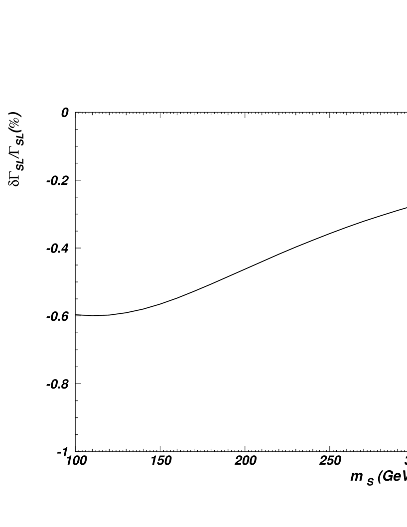
FIG. 2.: The relative correction as a function of $m_{S}$, while taking $m_{\tilde{g}}=200$ GeV and $\tan\beta=2$.

FIG. 3.: The relative correction as a function of $m_{\tilde{g}}$, while taking $m_{S}=100$ GeV and $\tan\beta=2$.

FIG. 4.: The relative correction as a function of $\tan\beta$, while taking $m_{S}=100$ GeV and $m_{\tilde{g}}=200$ GeV.

REFERENCES

• [1] CDF Collaboration, F.Abe et al., Phys. Rev. Lett. 74, 2626 (1995).
• [2] CDF Collaboration, F.Abe et al., Phys. Rev. D50, 2966 (1994).
• [3] D0 Collaboration, S.Abachi et al., Phys. Rev. Lett. 74, 2632 (1995).
• [4] A. Czarnecki, Phys. Lett. B252, 467 (1990).
C.S. Li, R.J. Oakes, and T.C. Yuan, Phys. Rev. D43, 3759 (1991).
• [5] A. Denner and T. Sack, Nucl. Phys. B358, 46 (1991).
G. Eilam, R.R. Mendel, R. Migneron and A. Soni, Phys. Rev. Lett. 66, 3105 (1991).
• [6] M. Beneke and V.M. Braun, Phys. Lett. B348, 531 (1995).
• [7] T. Mehen, Phys. Lett. B417, 353 (1998); B382, 267 (1996).
• [8] A. Czarnecki and K. Melnikov, hep-ph/9806244.
• [9] B. Grzadkowski and W. Hollik, Nucl. Phys. B384, 101 (1992)
A. Denner and A.H. Hoang, Nucl. Phys. B397, 483 (1993).
• [10] C.S. Li, J.M. Yang, and B.Q. Hu, Phys. Rev. D48, 5425 (1993).
J.M. Yang and C.S. Li, Phys. Lett. B320, 117 (1994).
• [11] F. Fujikawa, Prog. Theor. Phys. 61, 1186 (1979).
J.H. Kühn, Acta Phys. Pol. B12, 374 (1981).
J.H. Kühn and K. H. Streng, Nucl. Phys. B198, 71 (1982).
• [12] N. Cabibbo, G. Corbo, and L. Maiani, Nucl. Phys. B155, 93 (1979).
• [13] M. Jezabek and J.H. Kühn, Nucl. Phys. B314, 1 (1989); B320, 20 (1989); Phys. Lett. B207, 91 (1988).
• [14] A. Denner, Fortschr. Phys. 41, 307 (1993).
• [15] S. Sirlin, Phys. Rev. D22, 971 (1980).
W. J. Marciano and A. Sirlin, ibid. 22, 2695 (1980); 31, 213(E) (1985).
A. Sirlin and W.J. Marciano, Nucl. Phys. B 189, 442 (1981).
K.I. Aoki et.al., Prog. Theor. Phys. Suppl. 73, 1 (1982).
• [16] G. Passarino and M. Veltman, Nucl. Phys. B160, 151 (1979).
R. Mertig, M. Bohm and A. Denner, Comp. Phys. Comm. 64, 345 (1991).
• [17] For instance: Particle Data Group, Euro. Phys. J. C3, 1 (1998).
• [18] H.E. Haber and G.L. Kane, Phys.Rep. 117, 75(1985);
J.F. Gunion and H.E. Haber, Nucl. Phys. B272, 1(1986)
For a review see, e.g., J.F. Gunion, Higgs Hunter’s Guide (Addison-Wesley, Reading, MA, 1990).
• [19] CDF Collaboration, Phys. Rev. D56, R1357 (1997); Phys. Rev. Lett. 75, 618 (1995); Phys. Rev. Lett. 69, 3439 (1992).
D0 Collaboration, EPS-HEP Conf., Jerusalem (1997) Ref. 859.
• [20] D0 Collaboration, Fermilab Pub-96/449-E; Phys. Rev. Lett. 76, 2222 (1996).
Refer to caption