MPI/PhT/98–88
hep–ph/9811467
November 1998

RECENT DEVELOPMENTS IN THE STUDY OF UNSTABLE PARTICLE PROCESSES

Developments in the analysis of $W$ and quark propagators in the resonance region, and recent considerations concerning the mass and width of the Higgs boson are reviewed. Particular emphasis is placed on the instability of these fundamental particles, and on related issues of gauge dependence.

1 Introduction

We discuss two subjects:

1. Radiative Corrections to $W$ and Quark Propagators in the Resonance Region and Related Problems.

2. On the Mass and Width of the Higgs Boson.

We recall the conventional definitions for the mass and width of unstable vector bosons:

$$M^{2}=M_{0}^{2}+\mathop{\rm Re}\nolimits A(M^{2}),\qquad M\Gamma=-\frac{\mathop{\rm Im}\nolimits A(M^{2})}{1-\mathop{\rm Re}\nolimits A^{\prime}(M^{2})},$$ (1)

where $A(s)$ is the transverse self-energy. More fundamental definitions are based on the complex-valued position of the propagator’s pole:$\!{}^{{\bf?}}$

$$\bar{s}=M_{0}^{2}+A(\bar{s}),\qquad\bar{s}=m_{2}^{2}-im_{2}\Gamma_{2}.$$ (2)

We may identify the mass and width with $m_{2}$ and $\Gamma_{2}$. Taking the real and imaginary parts of Eq. (2), we find

$$m_{2}^{2}=M_{0}^{2}+\mathop{\rm Re}\nolimits A(\bar{s}),\qquad m_{2}\Gamma_{2}=-\mathop{\rm Im}\nolimits A(\bar{s}),$$ (3)

so that $\mathop{\rm Re}\nolimits A(\bar{s})$ plays the rôle of mass counterterm. In terms of $m_{2}$ and $\Gamma_{2}$ the Breit-Wigner (BW) resonance amplitude is proportional to $(s-m_{2}^{2}+im_{2}\Gamma_{2})^{-1}$. As $\bar{s}$ is the position of a singularity in the analytically continued $S$-matrix, it has the important property of being gauge invariant.

If $\Gamma_{2}/m_{2}={\cal O}(g^{2})$ is small, one may expand Eq. (3) in powers of $m_{2}\Gamma_{2}$ about $m_{2}^{2}$. One readily finds that the result agrees with Eq. (1) in next-to-leading order (NLO), but not beyond. Given $m_{2}$ and $\Gamma_{2}$, other definitions are possible. For example, in the $Z^{0}$ case,

$$m_{1}=\sqrt{m_{2}^{2}+\Gamma_{2}^{2}},\qquad\Gamma_{1}=\frac{m_{1}}{m_{2}}\Gamma_{2}$$ (4)

lead, to very good accuracy, to an $s$-dependent BW amplitude. An important consequence is that $m_{1}$ and $\Gamma_{1}$ can be identified with the $Z^{0}$ mass and width measured at LEP. A third frequently employed parametrization is

$$\bar{s}=\left(m_{3}-i\frac{\Gamma_{3}}{2}\right)^{2}.$$ (5)

Theoretical arguments led to the conclusion that, in the $Z^{0}$ case, $M$ is gauge dependent in ${\cal O}(g^{4})$ and higher.$\!{}^{{\bf?},{\bf?}}$ This has been confirmed by an analysis of the $Z^{0}$ resonant propagator in general $R_{\xi}$ gauge.$\!{}^{{\bf?},{\bf?}}$ The gauge dependence in ${\cal O}(g^{4})$ is small ($\,\hbox to0.0pt{\lower 3.5pt\hbox{$\mathchar 0\relax\sim$}\hss}\raise 1.0pt\hbox{$<$}\,2$ MeV), but it is unbounded in ${\cal O}(g^{6})$.

2 $W$ Propagator in the Resonance Region

A very recent work has extended the analysis to $W$ and quark propagators in the resonance region.$\!{}^{{\bf?}}$

One finds that a new problem emerges: in the treatment of the photonic corrections, conventional mass renormalization generates, in NLO, a series in powers of $M\Gamma/(s-M^{2})$, which does not converge in the resonance region! Furthermore, it diverges term-by-term at $s=M^{2}$. This problem is generally present whenever the unstable particle is coupled to massless quanta. Aside from the $W$, an interesting example is the QCD correction to a quark propagator when the weak interactions are switched on, so that the quark becomes unstable. A solution of this serious problem is presented in the framework of the complex pole formalism.$\!{}^{{\bf?}}$

In order to illustrate the difficulties emerging in the resonance region when conventional mass renormalization is employed, we consider the contribution of the transverse part of the $W$ propagator in the loop of Fig. 1, which contains $l$ self-energy insertions.

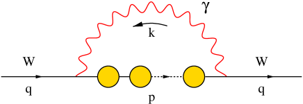
Figure 1: A class of photonic corrections to the $W$ self-energy. The inner solid and dashed lines and blobs represent transverse $W$ propagators and self-energies.

Calling

$$\Pi^{\scriptscriptstyle(T)}_{\mu\nu}(q)=t_{\mu\nu}(q)A(s),$$ (6)

the transverse $W$ self-energy, where $s\equiv q^{2}$ and $t_{\mu\nu}(q)=$ $g_{\mu\nu}-q_{\mu}q_{\nu}/q^{2}$, the contribution $A_{{\scriptscriptstyle W}\gamma}^{(l)}(s)$ from Fig. (1) to $A(s)$ is given by

$$A_{{\scriptscriptstyle W}\gamma}^{(l)}(s) = ie^{2}(\mu)\,\frac{t_{\mu\nu}(q)}{(n-1)}\,\mu^{4-n}$$

$$\times \!\!\!\!\!\!\!\!\!\!\!\!\int\frac{d^{n}\!k}{(2\pi)^{n}}{\cal{D}}^{{\scriptscriptstyle(}\gamma{\scriptscriptstyle)}}_{\rho\beta}(k){\cal{D}}^{\scriptscriptstyle(W,T)}_{\lambda\alpha}(p){\cal{V}}^{\rho\lambda\nu}{\cal{V}}^{\beta\alpha\mu}\left[\frac{A^{{\scriptscriptstyle(}s{\scriptscriptstyle)}}(p^{2})}{p^{2}-M^{2}+i\epsilon}\right]^{l},$$ (7)

where $p=q+k$ is the $W$ loop-momentum,

$${\cal D}^{{\scriptscriptstyle(}\gamma{\scriptscriptstyle)}}_{\rho\beta}(k)=-\frac{i}{k^{2}}\left(g_{\rho\beta}+(\xi_{\gamma}-1)\frac{k_{\rho}k_{\beta}}{k^{2}}\right),$$ (8)

$${\cal D}^{\scriptscriptstyle(W,T)}_{\lambda\alpha}(p)=\frac{-i}{p^{2}-M^{2}+i\epsilon}\left(g_{\alpha\lambda}-\frac{p_{\alpha}p_{\lambda}}{p^{2}}\right),$$ (9)

$${\cal V}^{\beta\alpha\mu}=(2p-k)^{\beta}g^{\alpha\mu}+(2k-p)^{\alpha}g^{\beta\mu}-(k+p)^{\mu}g^{\beta\alpha},$$ (10)

$\xi_{\gamma}$ is the photon gauge parameter and $A^{{\scriptscriptstyle(}s{\scriptscriptstyle)}}(p^{2})$ stands for the $W$ transverse self-energy with the conventional mass renormalization subtraction:

$$A^{{\scriptscriptstyle(}s{\scriptscriptstyle)}}(p^{2}) = \mbox{Re}\left(A(p^{2})-A(M^{2})\right)+i\mbox{Im}A(p^{2})$$ (11)

$$= A(p^{2})-A(M^{2})+i\mbox{Im}A(M^{2}).$$

We note that each insertion of $A^{{\scriptscriptstyle(}s{\scriptscriptstyle)}}(p^{2})$ is accompanied by an additional denominator $[p^{2}-M^{2}+i\epsilon]$. Thus, Eq. (7) may be regarded as the $l$th term in an expansion in powers of

$$\left[A(p^{2})-A(M^{2})+i\mbox{Im}A(M^{2})\right]\left(p^{2}-M^{2}+i\epsilon\right)^{-1}.$$

As $A(p^{2})-A(M^{2})=O[g^{2}(p^{2}-M^{2})]$ for $p^{2}\approx M^{2}$, the contribution $[A(p^{2})-A(M^{2})]$ $(p^{2}-M^{2}+i\epsilon)^{-1}$ is of $O(g^{2})$ throughout the region of integration. However, as $i\mbox{Im}A(M^{2})\approx-iM\Gamma$ is not subtracted, the combination $i\mbox{Im}A(M^{2})/(p^{2}-M^{2}+i\epsilon)$ may lead to terms of $O(1)$ if the domain of integration $|p^{2}-M^{2}|$ $\stackrel{{\scriptstyle\textstyle<}}{{\sim}}\,$$M\Gamma$ is important. In fact, the contribution of $[i\mbox{Im}A(M^{2})/(p^{2}-M^{2}+i\epsilon)]^{l}$ to Eq. (7) is, to leading order,

$$A_{{\scriptscriptstyle W}\gamma}^{(l)}(s)=\frac{(-iM\Gamma)^{l}}{l!}\frac{d^{l}}{d(M^{2})^{l}}A_{{\scriptscriptstyle W}\gamma}^{(0)}(s)+\ldots,$$ (12)

where $A_{{\scriptscriptstyle W}\gamma}^{(0)}(s)$ represents the diagram with no self-energy insertions and the dots indicate additional contributions not relevant to our argument.

In the resonance region $|s-M^{2}|$ $\stackrel{{\scriptstyle\textstyle<}}{{\sim}}\,$$M\Gamma$ the zeroth order propagator is inversely proportional to $(s-M^{2}+iM\Gamma)=O(g^{2})$. In NLO, contributions of $O[\alpha(s-M^{2}),\alpha M\Gamma]$ are therefore retained but those of $O[\alpha(s-M^{2})^{2}]$ are neglected. Explicit evaluation of $A_{{\scriptscriptstyle W}\gamma}^{(0)}(s)$ in NLO leads to

$$A_{{\scriptscriptstyle W}\gamma}^{(0)}(s)=\frac{\alpha}{2\pi}\left[(\xi_{\gamma}-3)(s-M^{2})\ln\!\left(\frac{M^{2}-s}{M^{2}}\right)+\ldots\right].$$ (13)

Inserting Eq. (13) into Eq. (12) we obtain

$$A_{{\scriptscriptstyle W}\gamma}^{(1)}(s) = \frac{\alpha}{2\pi}(\xi_{\gamma}-3)\left(iM\Gamma\right)\left[\ln\!\left(\frac{M^{2}-s}{M^{2}}\right)+\frac{s}{M^{2}}\right]+\ldots,$$

$$A_{{\scriptscriptstyle W}\gamma}^{(l)}(s) = \frac{\alpha}{2\pi}(\xi_{\gamma}-3)\frac{(s-M^{2})}{l(l-1)}\left(\frac{-iM\Gamma\phantom{{}^{2}}}{s-M^{2}}\right)^{\!l}+\ldots,\quad(l\geq 2).$$ (14)

As in the resonance region all these terms contribute in NLO, conventional mass renormalization leads in NLO to a series in powers of $M\Gamma/(s-M^{2})$, which does not converge in the resonance region. Rather than generating contributions of higher order in $g^{2}$, each successive self-energy insertion gives rise to a factor $-iM\Gamma/(s-M^{2})$, which is nominally of $O(1)$ in the resonance region and furthermore diverges at $s=M^{2}$! We note also that the use of Eq. (14) would lead to power-behaved infrared divergences in $\mathop{\rm Re}\nolimits A(M^{2})$ (mass counterterm) for $l=2,4,6,\ldots$, and in the width for $l=3,5,7,\ldots$.

One possibility would be to resum the series $\sum^{\infty}_{l=0}A_{{\scriptscriptstyle W}\gamma}^{(l)}(s)$ with $A_{{\scriptscriptstyle W}\gamma}^{(l)}(s)$ given by Eq. (12). This would lead to

$$\sum^{\infty}_{l=0}A_{{\scriptscriptstyle W}\gamma}^{(l)}(s,M^{2})=A_{{\scriptscriptstyle W}\gamma}^{(0)}(s,M^{2}-iM\Gamma)+\ldots,$$ (15)

or

$$\sum^{\infty}_{l=0}A_{{\scriptscriptstyle W}\gamma}^{(l)}(s)=\frac{\alpha}{2\pi}\left[(\xi_{\gamma}-3)(s-M^{2}+iM\Gamma)\ln\left(\frac{M^{2}-iM\Gamma-s}{M^{2}-iM\Gamma}\right)+\ldots\right].$$ (16)

Even if one accepts these resummations rather than the usual term by term expansions, the theoretical situation in the conventional formalism is very unsatisfactory. In fact, in the conventional formalism, the $W$ propagator is inversely proportional to

$${\cal D}^{-1}(s)=s-M^{2}+iM\Gamma-\left(A(s)-A(M^{2})\right)-iM\Gamma\,\mbox{Re}A^{\prime}(M^{2}),$$ (17)

where $\Gamma$ is the radiatively corrected width and we have employed its conventional expression

$$M\Gamma=-\mbox{Im}A(M^{2})/[1-\mbox{Re}A^{\prime}(M^{2})].$$ (18)

The contribution of the $(s-M^{2}+iM\Gamma)\ln[(M^{2}-iM\Gamma-s)/(M^{2}-iM\Gamma)]$ term to ${\cal D}^{-1}(s)$ is

$$-\frac{\alpha}{2\pi}(\xi_{\gamma}-3)\left[(s-M^{2}+iM\Gamma)\ln\left(\frac{M^{2}-iM\Gamma-s}{M^{2}-iM\Gamma}\right)+iM\Gamma\left(1+i\frac{\pi}{2}\right)\right]$$

and we note that the last term is a gauge-dependent contribution not proportional to the zeroth order term $s-M^{2}+iM\Gamma$. As a consequence, in NLO the pole position is shifted to ${\widetilde{M}}^{2}-i\widetilde{M}\widetilde{\Gamma}$, where

$${\widetilde{M}}^{2} = M^{2}[1-(\alpha/4)(\xi_{\gamma}-3)(\Gamma/M)],$$ (19)

$$\widetilde{\Gamma} = \Gamma[1-(\alpha/2\pi)(\xi_{\gamma}-3)].$$ (20)

As the pole position is gauge-invariant, so must be $\widetilde{M}$ and $\widetilde{\Gamma}$. Furthermore, in terms of $\widetilde{M}$ and $\widetilde{\Gamma}$, ${\cal D}^{-1}(s)$ retains the Breit-Wigner structure. Thus, in a resonance experiment $\widetilde{M}$ and $\widetilde{\Gamma}$ would be identified with the mass and width of $W$.

The relation $\widetilde{\Gamma}=\Gamma[1-(\alpha/2\pi)(\xi_{\gamma}-3)]$ leads to a contradiction: the measured, gauge-independent, width $\widetilde{\Gamma}$ would differ from the theoretical value $\Gamma$ by a gauge-dependent quantity in NLO! This contradicts the premise of the conventional formalism that $\Gamma$, defined in Eq. (18), is the radiatively corrected width and is, furthermore, gauge-independent. We can anticipate that the root of this clash between the resummed expression and the conventional definition of width is that the latter is only an approximation. In particular, it is not sufficiently accurate when non-analytic contributions are considered.

A good and consistent formalism may circumvent awkward resummations of non-convergent series and should certainly avoid the above discussed contradictions. To achieve this, we return to the transverse dressed $W$ propagator, inversely proportional to $p^{2}-M_{0}^{2}-A(p^{2})$. In the conventional mass renormalization one eliminates $M^{2}_{0}$ by means of the expression $M^{2}_{0}=M^{2}-\mbox{Re}A(M^{2})$ (Cf. Eq. (1)). An alternative possibility is to eliminate $M^{2}_{0}$ by means of $M^{2}_{0}=\overline{s}-A(\overline{s})$ (Cf. Eq. (2)). The dressed propagator in the loop integral is inversely proportional to $p^{2}-\overline{s}-[A(p^{2})-A(\overline{s})]$. Its expansion about $p^{2}-\overline{s}$ generates in Fig. (1) a series in powers of $[A(p^{2})-A(\overline{s})]/(p^{2}-\overline{s})$. As $A(p^{2})-A(\overline{s})=O[g^{2}(p^{2}-\overline{s})]$ when the loop momentum is in the resonance region, $[A(p^{2})-A(\overline{s})]/(p^{2}-\overline{s})$ is $O(g^{2})$ throughout the domain of integration. Thus, each successive self-energy insertion leads now to terms of higher order in $g^{2}$ without awkward non-convergent contributions. In this modified strategy, the zeroth order propagator in Eq. (9) is replaced by

$${\cal D}^{\scriptscriptstyle(W,T)}_{\alpha\lambda}(p)=\frac{-i}{p^{2}-\overline{s}}\left(g_{\alpha\lambda}-\frac{p_{\alpha}p_{\lambda}}{p^{2}}\right).$$ (21)

The poles in the $k^{0}$ complex plane remain in the same quadrants as in Feynman’s prescription and Feynman’s contour integration or Wick’s rotation can be carried out. $A_{{\scriptscriptstyle W}\gamma}^{(0)}(s)$, Fig. (1) without loop insertions, now leads directly to

$$A_{{\scriptscriptstyle W}\gamma}^{(0)}(s)=\frac{\alpha}{2\pi}\left[(\xi_{\gamma}-3)(s-\overline{s})\ln\!\left(\frac{\overline{s}-s}{\overline{s}}\right)+\ldots\right],$$ (22)

which has the same structure as the expression we obtained in the conventional approach after resumming a non-convergent series. $A_{{\scriptscriptstyle W}\gamma}^{(l)}(s)$ ($l\geq 1$), the contributions with $l$ insertions in Fig. (1), are now of $O(\alpha g^{2l})$, the normal situation in perturbative expansions. The $W$ propagator in the modified formalism is inversely proportional to $s-\overline{s}-[A(s)-A(\overline{s})]$. As $A_{{\scriptscriptstyle W}\gamma}^{(0)}(s)$ is now proportional to $s-\overline{s}$, the pole position is not displaced, the gauge-dependent contributions factorize as desired, and the above discussed pitfalls are avoided. $A_{{\scriptscriptstyle W}\gamma}^{(l)}(s)$ leads now to contributions to $[A(s)-A(\overline{s})]$ of order $O[(s-\overline{s})\alpha g^{2l}]=O[\alpha g^{2(l+1)}]$ in the resonance region and can therefore be neglected in NLO for $l\geq 1$. We note that the $\ln[(\overline{s}-s)/\overline{s}]$ term in Eq. (22) cancels for $\xi_{\gamma}=3$, the gauge introduced by Fried and Yennie in Lamb-shift calculations.$\!{}^{{\bf?}}$

The remaining contributions to $A(s)$ from the photonic diagrams, including those from the longitudinal part of the $W$ propagator in Fig. (1), and from the diagrams involving the unphysical scalars $\phi$ and the ghost $C_{\gamma}$, have no singularities at $s=M^{2}$ and can therefore be studied with conventional methods.

Calling $A^{\gamma}(s)$ the overall contribution of the one-loop photonic diagrams to the transverse $W$ self-energy, in the modified formulation the relevant quantity in the correction to the $W$ propagator is $A^{\gamma}(s)-A^{\gamma}(\overline{s})$. In general $R_{\xi}$ gauge, we find in NLO

$$A^{\gamma}(s)-A^{\gamma}(\overline{s})=\frac{\alpha(m_{2})}{2\pi}(s-\overline{s})\left\{\delta\left(\frac{\xi_{\scriptscriptstyle W}}{2}-\frac{23}{6}\right)+\frac{34}{9}-2\ln\!\left(\frac{\overline{s}-s}{\overline{s}}\right)\right.$$

$$\!\!\!\!\!\!\!\!\!\!-\left(\xi_{\scriptscriptstyle W}-1\right)\left[\frac{\xi_{\scriptscriptstyle W}}{12}-\left(1-\frac{(\xi_{\scriptscriptstyle W}-1)^{2}}{12}\right)\ln\!\left(\frac{\xi_{\scriptscriptstyle W}-1}{\xi_{\scriptscriptstyle W}}\right)\right]-\left(\frac{11}{12}-\frac{\xi_{\scriptscriptstyle W}}{4}\right)\ln\xi_{\scriptscriptstyle W}$$

$$\!\!\!\!\!\!\!\!\!\!\left.+\left(\xi_{\gamma}-1\right)\left[\frac{\delta}{2}+\frac{1}{2}+\ln\!\left(\frac{\overline{s}-s}{\overline{s}}\right)+\frac{(\xi_{\scriptscriptstyle W}^{2}-1)}{4}\ln\!\left(\frac{\xi_{\scriptscriptstyle W}-1}{\xi_{\scriptscriptstyle W}}\right)-\frac{\ln\xi_{\scriptscriptstyle W}}{4}+\frac{\xi_{\scriptscriptstyle W}}{4}\right]\right\},$$

where $\delta=(n-4)^{-1}+(\gamma_{E}-\ln 4\pi)/2$ and we have set $\mu=m_{2}$. Of particular interest in Eq. (LABEL:eq:Agamma-Agamma) is the log term

$$\frac{\alpha(m_{2})}{2\pi}\left(\xi_{\gamma}-3\right)\left(s-\overline{s}\right)\ln\!\left(\frac{\overline{s}-s}{\overline{s}}\right),$$

which is independent of $\xi_{\scriptscriptstyle W}$ but is proportional to $(\xi_{\gamma}-3)$. The logarithm $\ln(\xi_{\scriptscriptstyle W}-1)$ in Eq. (LABEL:eq:Agamma-Agamma) contains an imaginary contribution $-i\pi\theta(1-\xi_{\scriptscriptstyle W})$. This can be understood from the observation that, for $\xi_{\scriptscriptstyle W}<1$, a $W$ boson of mass $s=M^{2}$ has non-vanishing phase space to “decay” into a photon and particles of mass $M^{2}\xi_{\scriptscriptstyle W}$.

3 Gauge Dependence of the On-Shell Mass

The difference between the pole mass $m_{1}$, defined in Eq. (4), and the conventional on-shell mass $M$, defined in Eq. (1), is

$$M^{2}-m_{1}^{2}=\mbox{Re}A(M^{2})-\mbox{Re}A(\overline{s})-\Gamma_{2}^{2}.$$ (24)

The contribution of the $(s-\overline{s})\ln[(\overline{s}-s)/\overline{s}]$ term to the r.h.s. of Eq. (24) is

$$\frac{\alpha(m_{2})}{2\pi}\left(\xi_{\gamma}-3\right)\left[\left(M^{2}-m_{2}^{2}\right)\mbox{Re}\ln\!\left(\frac{\overline{s}-M^{2}}{\overline{s}}\right)-m_{2}\Gamma_{2}\mbox{Im}\ln\!\left(\frac{\overline{s}-M^{2}}{\overline{s}}\right)\right]$$ (25)

$$\approx \frac{\alpha(m_{2})}{2\pi}\left(\xi_{\gamma}-3\right)\left[\left(M^{2}-m_{1}^{2}\right)\mbox{Re}\ln\!\left(\frac{\overline{s}-M^{2}}{\overline{s}}\right)+m_{2}\Gamma_{2}\frac{\pi}{2}\right].$$

In $\mbox{Im}\ln[(\overline{s}-M^{2})/\overline{s}]$ we have approximated $M^{2}\approx m_{1}^{2}$ and used the fact that $\theta=-\pi/2$ for $s=m_{1}^{2}$. Thus, we have

$$M^{2}-m_{1}^{2}=\frac{\alpha(m_{2})}{4}(\xi_{\gamma}-3)m_{2}\Gamma_{2}+\ldots,$$ (26)

where the dots indicate additional contributions. We note that this last equation corresponds to our previous result from the propagator, Eq. (19), with the identification $\widetilde{M}\rightarrow m_{1}$. In particular, Eq. (26) leads to $m_{1}-M=\alpha(m_{2})\Gamma_{2}/4\approx 4\mbox{ MeV}$ in the frequently employed ’t Hooft-Feynman gauge $(\xi_{i}=1)$, and to $\approx 6\mbox{ MeV}$ in the Landau gauge $(\xi_{i}=0)$. The contribution to $M^{2}-m_{1}^{2}$ from the term proportional to $(s-\overline{s})(\xi_{\gamma}-1)(\xi_{\scriptscriptstyle W}^{2}-1)\ln(\xi_{\scriptscriptstyle W}-1)$ (Cf. Eq. (LABEL:eq:Agamma-Agamma)) is $(\alpha/8)(\xi_{\gamma}-1)M\Gamma(\xi_{\scriptscriptstyle W}^{2}-1)\,\theta(1-\xi_{\scriptscriptstyle W})$, which is unbounded in $\xi_{\gamma}$ but restricted to $\xi_{\scriptscriptstyle W}<1$. In analogy with the $Z$ case, there are also bounded gauge-dependent contributions to $m_{1}-M$ arising from non-photonic diagrams in the restricted range $M_{\scriptscriptstyle W}>M_{\scriptscriptstyle Z}\sqrt{\xi_{\scriptscriptstyle Z}}+M_{\scriptscriptstyle W}\sqrt{\xi_{\scriptscriptstyle W}}$ or $\sqrt{\xi}_{\scriptscriptstyle Z}\leq\cos\theta_{\mbox{\footnotesize{w}}}[1-\sqrt{\xi}_{\scriptscriptstyle W}]$, and from the photonic corrections proportional to $(\xi_{\scriptscriptstyle W}-1)\ln[(\xi_{\scriptscriptstyle W}-1)/\xi_{\scriptscriptstyle W}]$ (Cf. Eq. (LABEL:eq:Agamma-Agamma)).

The following observation is appropriate at this point. In calculating $\Delta r\$$\!{}^{{\bf?}}$ (and its $\overline{\rm MS}$ counterparts, $\Delta\hat{r}\$$\!{}^{{\bf?}}$ and $\Delta\hat{r}_{W}\$$\!{}^{{\bf?}}$), one must consider the $W$ mass counterterm. In the complex pole formalism, the mass counterterm is $\mathop{\rm Re}\nolimits A(\bar{s})$ and we see that the contribution from Eq. (22) vanishes exactly. If one employs instead the conventional mass counterterm $\mathop{\rm Re}\nolimits A(M^{2})$, the resummed expression of Eq. (16) gives an unbounded gauge-dependent contribution $(\alpha/4)(\xi_{\gamma}-3)M\Gamma$. The same result is obtained if one restricts one-self to $A_{{\scriptscriptstyle W}\gamma}^{(0)}+A_{{\scriptscriptstyle W}\gamma}^{(1)}$ (Cf. Eqs. (13) and (14)), rather than Eq. (16), and evaluates the imaginary part of the logarithm at $s=M^{2}$ using the $i\epsilon$ prescription. One should eliminate these gauge dependent terms by means of the replacement $M^{2}-(\alpha/4)(\xi_{\gamma}-3)M\Gamma=m_{1}^{2}$ and identify $m_{1}$ with the measured mass. On the other hand, if we again retain only $A_{{\scriptscriptstyle W}\gamma}^{(0)}+A_{{\scriptscriptstyle W}\gamma}^{(1)}$ but regulate the logarithm with an infinitesimal photon mass $\lambda$ when $s=M^{2}$, $A_{{\scriptscriptstyle W}\gamma}^{(1)}(M^{2})$ is purely imaginary, so that it does not contribute to $\mathop{\rm Re}\nolimits A(M^{2})$, and the above-mentioned gauge dependence in $\mathop{\rm Re}\nolimits A(M^{2})$ and Eq. (26) does not arise.

4 Overall Corrections to $W$ Propagator in the Resonance Region

In contrast with the photonic corrections, the non-photonic contributions $A_{np}(s)$ to $A(s)$ are analytic around $s=\overline{s}$. In NLO we can therefore write

$$A_{np}(s)-A_{np}(\overline{s})=(s-\overline{s})A_{np}^{\prime}(m_{2}^{2})+\ldots,$$ (27)

where the dots indicate higher-order contributions.

In the resonance region, and in NLO, the transverse $W$ propagator becomes

$${\cal D}^{\scriptscriptstyle(W,T)}_{\alpha\beta}(q)=\frac{-i\left(g_{\alpha\beta}-q_{\alpha}q_{\beta}/q^{2}\right)}{\left(s-\overline{s}\right)\left[1-A_{np}^{\prime}(m_{2}^{2})-\frac{\alpha(m_{2})}{2\pi}F(s,\overline{s},\xi_{\gamma},\xi_{\scriptscriptstyle W})\right]},$$ (28)

where $s=q^{2}$ and $F(s,\overline{s},\xi_{\gamma},\xi_{\scriptscriptstyle W})$ is the expression between curly brackets in Eq. (LABEL:eq:Agamma-Agamma). An alternative expression, involving an $s-$dependent width, can be obtained by splitting $A_{np}^{\prime}$ into real and imaginary parts, and the latter into fermionic Im$A^{\prime}_{f}$ and bosonic Im$A^{\prime}_{b}$ contributions. Neglecting very small scaling violations, we have

$$\mbox{Im}A^{\prime}_{f}(m_{2}^{2})\approx\mbox{Im}A_{f}(m_{2}^{2})/m_{2}^{2}\approx-\Gamma_{2}/m_{2}$$ (29)

and

$${\cal D}^{\scriptscriptstyle(W,T)}_{\alpha\beta}(q)=\frac{-i\left(g_{\alpha\beta}-q_{\alpha}q_{\beta}/q^{2}\right)}{\left(s-m_{1}^{2}+is\frac{\Gamma_{1}}{m_{1}}\right)\left[1-\mbox{Re}A_{np}^{\prime}(m_{1}^{2})-i\mbox{Im}A_{b}^{\prime}(m_{1}^{2})-\frac{\alpha(m_{1})}{2\pi}F\right]},$$ (30)

where $\Gamma_{1}/m_{1}=\Gamma_{2}/m_{2}$. $\mbox{Im}A_{b}^{\prime}(m_{1}^{2})$ is non-zero and gauge-dependent in the subclass of gauges that satisfy $\sqrt{\xi}_{\scriptscriptstyle Z}\leq\cos\theta_{\mbox{\footnotesize{w}}}[1-\sqrt{\xi}_{\scriptscriptstyle W}]$. Otherwise $\mbox{Im}A_{b}^{\prime}(m_{1}^{2})$ vanishes. Although $m_{1}$ and $\Gamma_{1}$ are gauge-invariant, $\mbox{Re}A^{\prime}_{np}(m_{1}^{2})$, $\mbox{Im}A^{\prime}_{np}(m_{1}^{2})$ and $F$ are gauge-dependent. In physical amplitudes, such gauge-dependent terms cancel against contributions from vertex and box diagrams. The crucial point is that the gauge-dependent contributions in Eq. (30) factorize so that such cancellations can take place and the position of the complex pole is not displaced.

5 QCD Corrections to Quark Propagators in the Resonance Region

In pure QCD quarks are stable particles, but they become unstable when weak interactions are switched on. As we anticipate similar problems to those in the $W$ case, we work from the outset in the complex pole formulation. Calling $\overline{m}=m-i\Gamma/2$ the position of the complex pole, $\Gamma$ arises from the weak interactions. If we treat $\Gamma$ to lowest order (LO), but otherwise neglect the remaining weak interactions contributions to the self-energy, the dressed quark propagator can be written

$$S^{\prime}_{F}(q\kern-4.49997pt{/})=\frac{i}{q\kern-4.49997pt{/}-\overline{m}-\left(\Sigma(q\kern-4.49997pt{/})-\Sigma(\overline{m})\right)},$$ (31)

where $\Sigma(q\kern-4.49997pt{/})$ is the pure QCD contribution. In NLO, in the resonance region, one finds

$$S^{\prime}_{F}(q\kern-4.49997pt{/})=\frac{i}{\left(q\kern-4.49997pt{/}-\overline{m}\right)}\left\{1-\frac{\alpha_{s}(m)}{3\pi}\left[2\left(\xi_{g}-3\right)\ln\!\left(\frac{\overline{m}^{2}-q^{2}}{\overline{m}^{2}}\right)+2\delta\xi_{g}\right]+\ldots\right\}^{-1},$$ (32)

where $\xi_{g}$ is the gluon gauge parameter and we have set $\mu=m$. As in the $W-$propagator case, we see that the logarithm vanishes in the Fried-Yennie gauge $\xi_{g}=3$.

6 Conclusions for First Subject

The conclusions can be summarized in the following points. i) Conventional mass renormalization, when applied to photonic and gluonic diagrams, leads to a series in powers of $M\Gamma/(s-M^{2})$ in NLO which does not converge in the resonance region. ii) In principle, this problem can be circumvented by a resummation procedure. iii) Unfortunately, the resummed expression leads to an inconsistent answer, when combined with the conventional definition of width. This is not too surprising, as the traditional expression of width treats the unstable particle as an asymptotic state, which is clearly only an approximation. iv) An alternative treatment of the resonant propagator is discussed, based on the complex-valued pole position $\overline{s}=M_{0}^{2}+A(\overline{s})$. The non-convergent series in the resonance region and the potential infrared divergences in $\Gamma$ and $M$ are avoided by employing $(p^{2}-\overline{s})^{-1}$ rather than $(p^{2}-M^{2})^{-1}$ in the Feynman integrals. The one-loop diagram leads now directly to the resummed expression of the conventional approach, while the multi-loop expansion generates terms which are genuinely of higher order. The non-analytic terms and the gauge-dependent corrections cause no problem because they are proportional to $s-\overline{s}$ and therefore exactly factorize. v) The presence of $\overline{s}$ in $\ln[(\overline{s}-s)/\overline{s}]$ removes the problem of apparent on-shell singularities. vi) The gauge dependence of the on-shell definition of mass for $W$ bosons present new features discussed in Section 3.

7 Differences Between the Pole and On-Shell Masses and Widths of the Higgs Boson

Eqs. (1–3) are also applicable to unphysical scalars. In this case, $A(s)$ is the corresponding self-energy. As explained in the Introduction, if one expands Eq. (3) in powers of $m_{2}\Gamma_{2}$ about $m_{2}^{2}$, the result agrees with Eq. (1) in NLO. The leading differences, which occur in next-to-next-to-leading order (NNLO), have been studied.$\!{}^{{\bf?}}$ One finds:

$$\frac{M-m_{2}}{m_{2}} = -\frac{\Gamma_{2}}{2m_{2}}\mathop{\rm Im}\nolimits A^{\prime}(m_{2}^{2})+{\cal O}(g^{6}),$$ (33)

$$\frac{\Gamma-\Gamma_{2}}{\Gamma_{2}} = \mathop{\rm Im}\nolimits A^{\prime}(m_{2}^{2})\left(\frac{\Gamma_{2}}{2m_{2}}+\mathop{\rm Im}\nolimits A^{\prime}(m_{2}^{2})\right)-\frac{m_{2}\Gamma_{2}}{2}\mathop{\rm Im}\nolimits A^{\prime\prime}(m_{2}^{2})+{\cal O}(g^{6}),$$

where $g^{2}$ is a generic coupling of ${\cal O}(\Gamma_{2}/m_{2})$. As the right-hand sides of Eq. (33) are of ${\cal O}(g^{4})$, we may evaluate them using the LO expressions for $\Gamma_{2}$, $\mathop{\rm Im}\nolimits A^{\prime}(m_{2}^{2})$, and $\mathop{\rm Im}\nolimits A^{\prime\prime}(m_{2}^{2})$.

In the Higgs-boson case, the one-loop bosonic contribution to $\mathop{\rm Im}\nolimits A(s)$ in the $R_{\xi}$ gauge is given by

$$\mathop{\rm Im}\nolimits A_{\rm bos}(s) = \frac{G}{4}s^{2}\left[-\left(1-\frac{4M_{W}^{2}}{s}+\frac{12M_{W}^{4}}{s^{2}}\right)\left(1-\frac{4M_{W}^{2}}{s}\right)^{1/2}\theta(s-4M_{W}^{2})\right.$$

$${}+\left.\left(1-\frac{M_{H}^{4}}{s^{2}}\right)\left(1-\frac{4\xi_{W}M_{W}^{2}}{s}\right)^{1/2}\theta(s-4\xi_{W}M_{W}^{2})+\frac{1}{2}(W\to Z)\right],$$

where $G=G_{\mu}/(2\pi\sqrt{2})$, $\xi_{W}$ is a gauge parameter, $(W\to Z)$ represents the sum of the preceding terms with the substitutions $M_{W}\to M_{Z}$ and $\xi_{W}\to\xi_{Z}$, and we have omitted gauge-invariant terms proportional to $\theta(s-4M_{H}^{2})$. The one-loop contribution due to a fermion $f$ is

$$\mathop{\rm Im}\nolimits A_{f}(s)=-\frac{G}{2}sN_{f}m_{f}^{2}\left(1-\frac{4m_{f}^{2}}{s}\right)^{3/2}\theta(s-4m_{f}^{2}),$$ (35)

where $N_{f}=1$ (3) for leptons (quarks). As expected, Eq. (7) is gauge invariant if $s=M_{H}^{2}$, but it depends on $\xi_{W}$ and $\xi_{Z}$ off-shell. The $\xi_{W}$ dependence in Eq. (7) is due to the fact that a Higgs boson of mass $s^{1/2}>2\xi_{W}^{1/2}M_{W}$ has non-vanishing phase space to “decay” into a pair of “particles” of mass $\xi_{W}^{1/2}M_{W}$. The first term in Eq. (7) can be verified by a very simple argument:$\!{}^{{\bf?}}$ in Eq. (7), only the unphysical scalar excitations have $M_{H}$-dependent couplings with the Higgs boson; therefore, if the unphysical particles decouple, which happens for $\xi_{W}>s/(4M_{W}^{2})$ and similarly for the $Z$ boson, $\mathop{\rm Im}\nolimits A(s)$ can be obtained by substituting $M_{H}^{2}\to s$ in the well-known expressions for the Higgs-boson partial widths multiplied by $M_{H}$. Using Eqs. (7) and (35), we find $\mathop{\rm Im}\nolimits A_{\rm bos}^{\prime}(m_{2}^{2})$, $\mathop{\rm Im}\nolimits A_{\rm bos}^{\prime\prime}(m_{2}^{2})$, $\mathop{\rm Im}\nolimits A_{\rm fer}^{\prime}(m_{2}^{2})$, and $\mathop{\rm Im}\nolimits A_{\rm fer}^{\prime\prime}(m_{2}^{2})$. This permits us to evaluate Eq. (33). We also wish to evaluate $(M^{\rm PT}-m_{2})/m_{2}$ and $(\Gamma^{\rm PT}-\Gamma_{2})/\Gamma_{2}$, where $M^{\rm PT}$ and $\Gamma^{\rm PT}$ are the pinch-technique (PT) on-shell mass and width obtained from Eq. (1) by employing the PT self-energy $a(s)$. We recall that the PT is a prescription that combines conventional self-energies with “pinch parts” from vertex and box diagrams in such a manner that the modified self-energies are independent of $\xi_{i}$ ($i=W,Z,\gamma$) and exhibit desirable theoretical properties.$\!{}^{{\bf?}}$ In the Higgs-boson case, $\mathop{\rm Im}\nolimits a(s)$ can be extracted from the literature.$\!{}^{{\bf?}}$

Figure 2: Relative deviations of $M$ and $\Gamma$ from $m_{2}$ and $\Gamma_{2}$, respectively, as functions of $\xi=\xi_{W}=\xi_{Z}$ in the $R_{\xi}$ gauge, assuming $m_{2}=800$ GeV. The horizontal lines across the figures indicate the corresponding deviations in the PT framework. The two abysses are associated with the unphysical thresholds $\xi=m_{2}^{2}/(4M_{Z}^{2}),m_{2}^{2}/(4M_{W}^{2})$, where the expansions in Eq. (33) obviously fail.

Identifying $M_{H}$ with $m_{2}$ and, for simplicity, setting $\xi=\xi_{W}=\xi_{Z}$, we have evaluated $(M-m_{2})/m_{2}$ and $(\Gamma-\Gamma_{2})/\Gamma_{2}$ as functions of $\xi$, for three values of $m_{2}$. We have employed $M_{W}=80.375$ GeV, $M_{Z}=91.1867$ GeV, and $m_{t}=175.6$ GeV, and have neglected contributions from fermions other than the top quark. For small Higgs mass ($m_{2}=200$ GeV), we find that, aside from the neighborhoods of unphysical thresholds where the expansion of Eq. (33) fails, $M$ and $\Gamma$ remain numerically very close to $m_{2}$ and $\Gamma_{2}$. In the intermediate case ($m_{2}=400$ GeV), the relative differences reach 0.6% in the mass and 3.3% in the width. However, for a heavy Higgs boson ($m_{2}=800$ GeV), the differences become very large, reaching 11% in the mass and 44% in the width (see Fig. 2). The largest differences occur for $\xi>m_{2}^{2}/(4M_{W}^{2})$, i.e., when the unphysical excitations decouple, a range that includes the unitary gauge. We recall that the latter retains only the physical degrees of freedom and, in this sense, it may be regarded as the most physical of all gauges. The large effects can be easily understood from Eq. (7). If $\xi>s/(4M_{W}^{2})$, the second term in Eq. (7) does not contribute, so that $\mathop{\rm Im}\nolimits A_{\rm bos}(s)\propto s^{2}$. For a heavy Higgs boson, this implies large values of $\mathop{\rm Im}\nolimits A^{\prime}(m_{2}^{2})$ and $\mathop{\rm Im}\nolimits A^{\prime\prime}(m_{2}^{2})$. For $\xi<s/(4M_{Z}^{2})$, the gauge-dependent terms contribute and cancel the leading $s^{2}$ dependence of $\mathop{\rm Im}\nolimits A_{\rm bos}(s)$, so that the magnitudes of $\mathop{\rm Im}\nolimits A^{\prime}(m_{2}^{2})$ and $\mathop{\rm Im}\nolimits A^{\prime\prime}(m_{2}^{2})$ drop sharply and the differences become much smaller. Of course, the 44% effect in the width for $\xi>m_{2}^{2}/(4M_{W}^{2})$ may cast doubts on the convergence of the expansions in Eq. (33). We interpret this finding as an indication of large corrections rather than a precise evaluation of $(\Gamma-\Gamma_{2})/\Gamma_{2}$.

Our results go beyond those reported in the literature.$\!{}^{{\bf?},{\bf?},{\bf?},{\bf?}}$ The reason is easy to understand: in these papers,$\!{}^{{\bf?},{\bf?},{\bf?},{\bf?}}$ the limits $M_{W}\to 0$ and $g\to 0$ are simultaneously considered keeping the Higgs self-coupling $\lambda\propto g^{2}M_{H}^{2}/M_{W}^{2}$ fixed. If the gauge parameter $\xi$ is also kept fixed, the gauge dependence of Eq. (7) is lost, and one obtains an $s$-independent result for $\mathop{\rm Im}\nolimits A_{\rm bos}(s)$, which does not contribute to the right-hand sides of Eq. (33). Thus, the above approximation, although interesting and useful, does not exhibit the gauge dependence and the large effects discussed here.

From the horizontal lines across Fig. 2, we see that the PT mass and width remain very close to $m_{2}$ and $\Gamma_{2}$, the maximum departures being 0.7% for $M^{\rm PT}$ and $-0.7\%$ for $\Gamma^{\rm PT}$. The differences vary somewhat if $M$ and $\Gamma$ are compared with $m_{1}$ and $\Gamma_{1}$. Through ${\cal O}(g^{6})$, $(M-m_{1})/m_{1}$ and $(\Gamma-\Gamma_{1})/\Gamma_{1}$ are obtained from $(M-m_{2})/m_{2}$ and $(\Gamma-\Gamma_{2})/\Gamma_{2}$ by subtracting the gauge-invariant term $\Gamma_{2}^{2}/(2m_{2}^{2})$. For $m_{2}=800$ GeV, $(M-m_{1})/m_{1}$ and $(\Gamma-\Gamma_{1})/\Gamma_{1}$ amount to 5.6% and 38% in the unitary gauge (rather than 11% and 44%) and to $-4.8\%$ and $-6.6\%$ in the ’t Hooft-Feynman gauge (rather than 0.9% and $-0.8\%$). For the same value of $m_{2}$, the differences $(M^{\rm PT}-m_{1})/m_{1}$ and $(\Gamma^{\rm PT}-\Gamma_{1})/\Gamma_{1}$ are $-5.1\%$ and $-6.5\%$ (rather than 0.7% and $-0.7\%$).

8 Mass and Width of a Heavy Higgs Boson

As the gauge-dependent effects in the width and the mass occur in NNLO, one would like to examine what happens when the widths, rather than differences, are evaluated to this order.$\!{}^{{\bf?}}$ Such calculations are, in fact, available in the recent literature in the heavy-Higgs approximation (HHA): $g\to 0$, $M_{W}\to 0$, with the Higgs quartic coupling $\lambda\propto g^{2}M_{H}^{2}/M_{W}^{2}$ fixed. What happens to the gauge dependence in this limit?

For finite values of the gauge parameters, $\xi_{W}$ and $\xi_{Z}$, $\xi_{W}M_{W}^{2},\xi_{Z}M_{Z}^{2}\to 0$ as $M_{W}^{2},M_{Z}^{2}\to 0$. Therefore, the second term in Eq. (7) contributes and cancels the leading $s$ dependence of the first one. Thus, for finite values of $\xi_{W}$ and $\xi_{Z}$, one obtains in the HHA

$$\mathop{\rm Im}\nolimits A(s)=-\frac{3}{8}GM^{4}\qquad\mbox{($R_{\xi}$ gauge)},$$ (36)

independent of $s$. Denoting by $M_{\xi}$ and $\Gamma_{\xi}$ the on-shell mass and width in the $R_{\xi}$ gauge (defined for finite values of $\xi_{W}$ and $\xi_{Z}$) and applying henceforth the HHA, Eqs. (33) and (36) lead to

$$\frac{M_{\xi}}{m_{2}}=1+{\cal O}(\lambda^{3}),\qquad\frac{\Gamma_{\xi}}{\Gamma_{2}}=1+{\cal O}(\lambda^{3}).$$ (37)

Instead, in the unitary gauge, one first takes the limit $\xi_{W},\xi_{Z}\to\infty$, in which case the term proportional to $\theta(s-4\xi_{W}M_{W}^{2})$ in Eq. (7) does not contribute, and one finds

$$\mathop{\rm Im}\nolimits A(s)=-\frac{3}{8}Gs^{2}\qquad\mbox{(unitary gauge)}.$$ (38)

Denoting by $M_{u}$ and $\Gamma_{u}$ the on-shell quantities in the unitary gauge, Eqs. (33) and (38) tell us that

$$\frac{M_{u}}{m_{2}}=1+\frac{9}{64}G^{2}m_{2}^{4}+{\cal O}(\lambda^{3}),\qquad\frac{\Gamma_{u}}{\Gamma_{2}}=1+\frac{9}{16}G^{2}m_{2}^{4}+{\cal O}(\lambda^{3}).$$ (39)

Comparison of Eq. (37) with Eq. (39) shows that, in the HHA, the leading gauge dependence of the on-shell mass or width reduces to a discontinuous function, with one value corresponding to finite $\xi_{W}$ and $\xi_{Z}$, and the other one to the unitary gauge. It should be pointed out, however, that for finite and large values of $\xi_{W}$ and $\xi_{Z}$, the limit $\xi_{W}M_{W}^{2},\xi_{Z}M_{Z}^{2}\to 0$ is not realistic within the SM, and must be regarded as a special feature of the HHA.

The relation between $\Gamma_{3}$ and $m_{3}$ was first obtained in NNLO by Ghinculov and Binoth,$\!{}^{{\bf?}}$ with a numerical evaluation of the expansion coefficients. We have independently derived this expansion. The relation between $m_{3}$ and $M_{\xi}$ was first given analytically in NNLO by Willenbrock and Valencia,$\!{}^{{\bf?}}$ an expansion that we have also verified. As the connection between the three pole parametrizations $(m_{1},\Gamma_{1})$, $(m_{2},\Gamma_{2})$, and $(m_{3},\Gamma_{3})$ is known exactly from Eqs. (2)–(5), and the relations of $(M_{\xi},\Gamma_{\xi})$ and $(M_{u},\Gamma_{u})$ with $(m_{2},\Gamma_{2})$ are given to the required accuracy in Eqs. (37) and (39), we readily find in NNLO the expansions of $\Gamma_{i}$ ($i=1,2,3,\xi,u$) in terms of $m_{i}$ in the three pole and two on-shell schemes discussed above to be

$$\Gamma_{i}=\frac{3}{8}Gm_{i}^{3}\left[1+a\frac{Gm_{i}^{2}}{\pi}+b_{i}\left(\frac{Gm_{i}^{2}}{\pi}\right)^{2}\right],$$ (40)

where

$$a = \frac{5}{4}\zeta(2)-\frac{3}{4}\pi\sqrt{3}+\frac{19}{8},\qquad b_{2}=b_{\xi}=0.96923(13),$$

$$b_{1} = b_{2}-\frac{9\pi^{2}}{64},\qquad b_{3}=b_{2}-\frac{9\pi^{2}}{128},\qquad b_{u}=b_{2}+\frac{9\pi^{2}}{64}.$$ (41)

For the ease of notation, we have put $m_{\xi}=M_{\xi}$ and $m_{u}=M_{u}$. Here, we have adopted the value for $b_{\xi}$ from Frink et al.$\!{}^{{\bf?}}$ It slightly differs from the value $0.97103(48)$.$\!{}^{{\bf?},{\bf?}}$ Although the difference is larger than the estimated errors, it amounts to less than 0.7% in the coefficients $b_{i}$, which is unimportant for our purposes. On the other hand, $m_{i}$ ($i=1,3,\xi,u$) are related to $m_{2}$ by

$$m_{i}=m_{2}\left[1+c_{i}\left(\frac{Gm_{2}^{2}}{\pi}\right)^{2}+d_{i}\left(\frac{Gm_{2}^{2}}{\pi}\right)^{3}\right],$$ (42)

where

$$c_{1} = \frac{9\pi^{2}}{128},\qquad c_{3}=\frac{9\pi^{2}}{512},\qquad c_{\xi}=0,\qquad c_{u}=\frac{9\pi^{2}}{64},$$

$$d_{1} = \frac{9\pi^{2}}{64}a,\qquad d_{3}=\frac{9\pi^{2}}{256}a,\qquad d_{\xi}=\frac{9\pi^{2}}{128}\left[-\frac{5}{4}\zeta(2)+\frac{\pi}{3}\sqrt{3}+\frac{7}{8}\right],$$ (43)

while $d_{u}$ is currently unknown. In the case of $i=3$, Eq. (40) agrees with Eq. (10) of Ref. 17 up to the numerical difference in $b_{3}$ discussed above.

Figure 3: Higgs-boson widths $\Gamma_{i}$ ($i=1,2,3,\xi,u$) as functions of the corresponding masses $m_{i}$ in the various pole and on-shell schemes. The down-most and middle solid lines correspond to the LO and NLO results, which are common to all renormalization schemes, while the up-most one refers to the NNLO result for $i=2,\xi$.

We see from Eq. (40) that all the width expansions have the same LO and NLO coefficients. This is due to the fact that the on-shell and pole widths only differ in NNLO$\!{}^{{\bf?}}$ and that the relations (42) among the masses do not involve terms linear in $Gm_{2}^{2}/\pi$. It is also interesting to note that the on-shell mass $M_{\rm PT}$ and width $\Gamma_{\rm PT}$, defined in terms of the PT$\!{}^{{\bf?}}$ self-energy, obey Eq. (40) with $b_{\rm PT}=b_{\xi}$, and Eq. (42) with $c_{\rm PT}=c_{\xi}=0$,$\!{}^{{\bf?}}$ while $d_{\rm PT}$ is currently unknown. In Fig. 3, the NNLO results for $\Gamma_{i}$ are plotted versus $m_{i}$ for the five cases considered in Eq. (40). The down-most and middle solid curves depict the LO and NLO expansions, respectively, which are common to the five cases. The up-most solid curve corresponds to the NNLO expansion for $i=2,\xi$. We note that $b_{1}$ is negative, while the other coefficients $b_{i}$ are positive. In particular, the NLO and NNLO corrections to $\Gamma_{1}(m_{1})$ cancel at $m_{1}=1.415$ TeV.

The comparison between the masses and widths in the various on-shell and pole schemes is particularly simple in the HHA:

$$\frac{m_{i}-m_{2}}{m_{2}} = c_{i}\left(\frac{Gm_{2}^{2}}{\pi}\right)^{2}+{\cal O}(\lambda^{3}),$$

$$\frac{\Gamma_{i}-\Gamma_{2}}{\Gamma_{2}} = (b_{i}+3c_{i}-b_{2})\left(\frac{Gm_{2}^{2}}{\pi}\right)^{2}+{\cal O}(\lambda^{3}).$$ (44)

These expressions lead immediately to Eq. (37), identical results for $M^{\rm PT}/m_{2}$ and $\Gamma^{\rm PT}/\Gamma_{2}$, and to Eq. (39). They also lead to

$$\frac{m_{3}}{m_{2}} = 1+\frac{9}{512}G^{2}m_{2}^{4},\qquad\frac{\Gamma_{3}}{\Gamma_{2}}=1-\frac{9}{512}G^{2}m_{2}^{4},$$

$$\frac{m_{1}}{m_{2}} = 1+\frac{9}{128}G^{2}m_{2}^{4},\qquad\frac{\Gamma_{1}}{\Gamma_{2}}=1+\frac{9}{128}G^{2}m_{2}^{4}.$$ (45)

For large $m_{2}$, these expressions approximate rather well the numerical results from the full SM. For instance, from Eq. (39) we have $(M_{u}-m_{2})/m_{2}=9.9\%$ and $(\Gamma_{u}-\Gamma_{2})/\Gamma_{2}=39.7\%$ for $m_{2}=800$ GeV, instead of 11% and 44%, respectively, from the full theory.

In order to analyze the scheme dependence of the above relations and the convergence properties of the corresponding perturbative series, one possible approach$\!{}^{{\bf?}}$ is to expand the relevant physical quantities in terms of different masses $m_{i}$. We illustrate this procedure with $m_{2}$ and $\Gamma_{2}$, which are the physical quantities that parametrize the conventional Breit-Wigner resonance amplitude, proportional to $(s-m_{2}^{2}+im_{2}\Gamma_{2})^{-1}$. The relation $\Gamma_{2}(m_{2})$ can be obtained directly from Eq. (40) or, via Eqs. (40) and (42), from the expansions

$$m_{2} = m_{i}\left[1-c_{i}\left(\frac{Gm_{i}^{2}}{\pi}\right)^{2}-d_{i}\left(\frac{Gm_{i}^{2}}{\pi}\right)^{3}\right],$$ (46)

$$\Gamma_{2} = \frac{3}{8}Gm_{i}^{3}\left[1+a\frac{Gm_{i}^{2}}{\pi}+(b_{2}-3c_{i})\left(\frac{Gm_{i}^{2}}{\pi}\right)^{2}\right].$$ (47)

In the $m_{i}$-expansion scheme, for given $m_{2}$, one evaluates $m_{i}$ from Eq. (46) and $\Gamma_{2}$ from Eq. (47). As the calculation of $\Gamma_{2}(m_{i})$ through ${\cal O}(\lambda^{n})$ only requires the knowledge of $m_{2}(m_{i})$ through ${\cal O}(\lambda^{n-1})$ and there is no term linear in $\lambda$ in Eq. (46), in LO (NLO), we set $m_{i}=m_{2}$ and keep the first contribution (first and second contributions) in Eq. (47), while in NNLO we retain the first two terms in Eq. (46) and the three terms in Eq. (47). In this manner, $m_{2}$ and $\Gamma_{2}$ are expanded to the same order in $\lambda$ relative to their respective Born approximations. Using as criterion of convergence the range throughout which the NNLO corrections are smaller in magnitude than the NLO ones at fixed $m_{2}$, we find that the domains of convergence for the $m_{1}$, $m_{2}$, $m_{3}$, $M_{\xi}$, and $M_{u}$ expansions are $m_{2}<733$ GeV, 930 GeV, 843 GeV, 930 GeV, and 672 GeV, respectively. In this connection, NLO (NNLO) correction means the difference between NLO and LO (NNLO and NLO) calculations. We also find that these expansions, when restricted to overlapping domains of convergence, are in good agreement with each other. Thus, the scheme dependence of the $\Gamma_{2}(m_{2})$ relation is quite small over the convergence domains of the expansions.

Another criterion that can be applied to judge the relative merits of the expansions is the closeness of the corresponding masses $m_{i}$ to $\bar{m}$, the peak position of the modulus of the $J=0$, iso-scalar Goldstone-boson scattering amplitude. The relation between $\bar{m}$ and $m_{3}$ is given to NNLO in the literature.$\!{}^{{\bf?}}$ Using Eq. (42), we can get the corresponding expressions for $i=1,2,\xi$. In the case of $i=2$, we have

$$m_{2}=\bar{m}\left[1+\frac{3\pi^{2}}{64}\left(\ln 2-\frac{5}{2}\right)\left(\frac{G\bar{m}^{2}}{\pi}\right)^{2}-0.778\left(\frac{G\bar{m}^{2}}{\pi}\right)^{3}\right].$$ (48)

For $\bar{m}=800$ GeV, we find $m_{1}=0.984\,\bar{m}$, $m_{2}=0.925\,\bar{m}$, $m_{3}=0.940\,\bar{m}$, and $M_{\xi}=0.934\,\bar{m}$, while, for $\bar{m}=1$ TeV, we have $m_{1}=0.954\,\bar{m}$, $m_{2}=0.797\,\bar{m}$, $m_{3}=0.836\,\bar{m}$, and $M_{\xi}=0.829\,\bar{m}$.

9 Conclusions for Second Subject

i) In the SM, for a heavy Higgs boson, the differences between the on-shell mass and width and their pole counterparts $(m_{2},\Gamma_{2})$ are sensitive functions of the gauge parameter. They become numerically large over a class of gauges that includes the unitary gauge (about 11% in the mass and 44% in the width for $m_{2}=800$ GeV). These features were overlooked in the extensive literature on the Higgs boson. ii) For a light Higgs boson ($M_{H}\approx 200$ GeV), the differences remain small in all gauges, except in the vicinity of unphysical thresholds, where our expansion is not valid. iii) In the intermediate case ($M_{H}\approx 400$ GeV), the differences reach 0.6% in the mass and 3.3% in the width. iv) The PT mass and width remain close to $(m_{2},\Gamma_{2})$, reaching differences of 0.7% and $-0.7\%$, respectively, at $m_{2}=800$ GeV. v) The differences of $M$, $M^{\rm PT}$, $\Gamma$, $\Gamma^{\rm PT}$ with $(m_{1},\Gamma_{1})$ are somewhat larger. vi) Theoretical expressions that relate the widths to the masses in NNLO are available in the HHA $(g\to 0$, $M_{W}\to 0$, $\lambda\propto g^{2}M_{H}^{2}/M_{W}^{2}$ fixed). This is precisely the order of expansion in which the gauge dependence sets in. vii) In the HHA, the gauge dependence is reduced to a two-valued expression, with one value corresponding to finite $\xi_{W}$, $\xi_{Z}$ ($R_{\xi}$ gauges), and another one corresponding to the unitary gauge. The theoretical expressions for the mass and width differences become very simple, and approximate rather well those obtained, for a heavy Higgs, in the full SM. viii) Using a convergence criterion based on the $(m_{2},\Gamma_{2})$ relation, the $m_{i}$-expansions have domains of convergence with upper bounds $(m_{2})_{\rm max}$ in the range 672 GeV${}<(m_{2})_{\rm max}<930$ GeV, depending on what masses are employed. The scheme dependence in the $(m_{2},\Gamma_{2})$ relation is small (${}\,\hbox to0.0pt{\lower 3.5pt\hbox{$\mathchar 0\relax\sim$}\hss}\raise 1.0pt\hbox{$<$}\,3\%$) over overlapping domains of convergence, but not beyond. Another criterion to judge the merits of the various expansion schemes is the relative proximity of the corresponding masses to the peak energy. ix) The fundamental importance of expansions based on the complex-pole parameters is that they involve gauge-invariant quantities, namely masses and widths that can be identified with physical quantities.

References

References

- [1] M. Consoli and A. Sirlin, in Physics at LEP, CERN 86–02, Vol. 1, p. 63 (1986); S. Willenbrock and G. Valencia, Phys. Lett. B 259, 373 (1991); R. G. Stuart, Phys. Lett. B 262, 113 (1991); Phys. Rev. Lett. 70, 3193 (1993); H. Veltman, Z. Phys. C 62, 35 (1994).
- [2] A. Sirlin, Phys. Rev. Lett. 67, 2127 (1991).
- [3] A. Sirlin, Phys. Lett. B 267, 240 (1991).
- [4] M. Passera and A. Sirlin, Phys. Rev. Lett. 77, 4146 (1996).
- [5] A. Sirlin, in Proceedings of the Ringberg Workshop: The Higgs Puzzle—What can we learn from LEP2, LHC, NLC and FMC?, Ringberg Castle, Germany, 8–13 December 1996, edited by B. A. Kniehl (World Scientific, Singapore, 1997) p. 39.
- [6] M. Passera and A. Sirlin, Phys. Rev. D 58, 113010 (1998); Acta Phys. Polon. B 29, 2901 (1998).
- [7] H. M. Fried and D. R. Yennie, Phys. Rev. 112, 1391 (1958).
- [8] A. Sirlin, Phys. Rev. D 22, 971 (1980).
- [9] A. Sirlin, Phys. Lett. B 232, 123 (1989); G. Degrassi, S. Fanchiotti, and A. Sirlin, Nucl. Phys. B 351, 49 (1991).
- [10] S. Fanchiotti and A. Sirlin, Phys. Rev. D 41, 319 (1990).
- [11] B. A. Kniehl and A. Sirlin, Phys. Rev. Lett. 81, 1373 (1998).
- [12] J. M. Cornwall, Phys. Rev. D 26, 1453 (1982); J. M. Cornwall and J. Papavassiliou, Phys. Rev. D 40, 3474 (1989); J. Papavassiliou, Phys. Rev. D 41, 3179 (1990); G. Degrassi and A. Sirlin, Phys. Rev. D 46, 3104 (1992).
- [13] A. Pilaftsis, Nucl. Phys. B 504, 61 (1997).
- [14] G. Valencia and S. Willenbrock, Phys. Rev. D 46, 2247 (1992); K. Riesselmann and S. Willenbrock, Phys. Rev. D 55, 311 (1997); T. Binoth and A. Ghinculov, Phys. Rev. D 56, 3147 (1997).
- [15] S. Willenbrock and G. Valencia, Phys. Lett. B 247, 341 (1990).
- [16] A. Ghinculov, Nucl. Phys. B 455, 21 (1995).
- [17] A. Ghinculov and T. Binoth, Phys. Lett. B 394, 139 (1997).
- [18] B. A. Kniehl and A. Sirlin, Preprint No. MPI/PhT/98–056 and hep–ph/9807545, Phys. Lett. B (in press).
- [19] A. Frink, B. A. Kniehl, D. Kreimer, and K. Riesselmann, Phys. Rev. D 54, 4548 (1996).