MPI/PhT/98–87
hep–ph/9811466
November 1998

DECOUPLING RELATIONS, EFFECTIVE LAGRANGIANS AND LOW-ENERGY THEOREMS

If QCD is renormalized by minimal subtraction (MS), at higher orders, the strong coupling constant $\alpha_{s}$ and the quark masses $m_{q}$ exhibit discontinuities at the flavour thresholds, which are controlled by so-called decoupling constants, $\zeta_{g}$ and $\zeta_{m}$, respectively. Adopting the modified MS ($\overline{\mbox{MS}}$) scheme, we derive simple formulae which reduce the calculation of $\zeta_{g}$ and $\zeta_{m}$ to the solution of vacuum integrals. This allows us to evaluate $\zeta_{g}$ and $\zeta_{m}$ through three loops. We also establish low-energy theorems, valid to all orders, which relate the effective couplings of the Higgs boson to gluons and light quarks, due to the virtual presence of a heavy quark $h$, to the logarithmic derivatives w.r.t. $m_{h}$ of $\zeta_{g}$ and $\zeta_{m}$, respectively. We also consider the effective QCD interaction of a CP-odd Higgs boson and verify the Adler-Bardeen nonrenormalization theorem at three loops.

1 Introduction

It is generally believed that quantum chromodynamics (QCD) is the true theory of the strong interactions. There are still open questions, concerning the origin of confinement or as to why the quark masses $m_{q}$ and the asymptotic scale parameter $\Lambda$ have the values they happen to have. The answers to these questions probably lie outside the scope of perturbative QCD, which forms the basis of this presentation. In perturbative QCD, the strong coupling constant $\alpha_{s}=g^{2}/(4\pi)$, where $g$ is the gauge coupling, is small enough to serve as a useful expansion parameter, and quarks and gluons may appear as asymptotic states of the scattering matrix.

QCD is a nonabelian Yang-Mills theory based on the gauge group SU(3). In the covariant gauge, the Lagrangian reads

$${\cal L} = \sum_{q=1}^{n_{f}}\bar{\psi}_{q}^{i}\left(i\;/\!\!\!\!D^{ij}-\delta^{ij}m_{q}\right)\psi_{q}^{j}-\frac{1}{4}\left(G_{\mu\nu}^{a}\right)^{2}-\frac{1}{2\xi}\left(\partial^{\mu}G_{\mu}^{a}\right)^{2}+\left(\partial^{\mu}\bar{c}^{a}\right)\nabla_{\mu}^{ab}c^{b},$$

$$D_{\mu}^{ij} = \delta^{ij}\partial_{\mu}-ig[T^{a}]^{ij}G_{\mu}^{a},\qquad\nabla_{\mu}^{ab}=\delta^{ab}\partial_{\mu}-gf^{abc}G_{\mu}^{c},$$

$$G_{\mu\nu}^{a} = \partial_{\mu}G_{\nu}^{a}-\partial_{\nu}G_{\mu}^{a}+gf^{abc}G_{\mu}^{b}G_{\nu}^{c},$$ (1)

with $n_{f}=6$ flavours of quarks $\psi_{q}^{i}$ ($i=1,2,3$), gluons $G_{\mu}^{a}$ ($a=1,\ldots,8$), Faddeev-Popov ghosts $c^{a}$, and gauge parameter $\xi$. The generators $T^{a}$ satisfy the commutation relations $[T^{a},T^{b}]=if^{abc}T^{c}$, where $f^{abc}$ are the structure constants.

In the calculation of QCD quantum corrections, one generally encounters, among other things, ultraviolet (UV) divergences, which must be regularized and removed by renormalization. In quantum electrodynamics, it is natural to employ the on-shell renormalization scheme, where the fine-structure constant is renormalized in the limit of the photon being on its mass shell. Due to confinement, this limit cannot be taken in QCD, and it is natural to employ the most convenient renormalization scheme instead. It has become customary to use dimensional regularization$\!{}^{{\bf?}}$ in connection with minimal subtraction (MS).$\!{}^{{\bf?}}$ I.e., the integrations over the loop momenta are performed in $D=4-2\epsilon$ space-time dimensions, introducing a ’t Hooft mass scale $\mu$ to keep the (renormalized) coupling constant dimensionless. The poles in $\epsilon$ that emerge as UV divergences in the physical limit $\epsilon\to 0$ are then combined with the bare (UV-divergent) parameters and fields in Eq. (1) so as to render them renormalized (UV finite). This is always possible because QCD is a renormalizable theory. In the modified MS ($\overline{\rm MS}$) scheme,$\!{}^{{\bf?}}$ the specific combination of transcendental numbers that always appears along with the poles in $\epsilon$ is also subtracted. In the following, bare quantities will be denoted by the superscript ‘0.’ Specifically, we have

$$g^{0} = \mu^{\epsilon}Z_{g}g(\mu),\qquad m_{q}^{0}=Z_{m}m_{q}(\mu),\qquad\xi^{0}-1=Z_{3}(\xi(\mu)-1),$$

$$\psi_{q}^{0,i} = \sqrt{Z_{2}}\psi_{q}^{i}(\mu),\qquad G_{\mu}^{0,a}=\sqrt{Z_{3}}G_{\mu}^{a}(\mu),\qquad c^{0,a}=\sqrt{\tilde{Z}_{3}}c^{a}(\mu).$$ (2)

In the MS-like schemes, the renormalization constants $Z$ may be written in the simple form

$$Z=1+\sum_{i=1}^{\infty}\sum_{j=1}^{i}Z_{ij}\frac{a^{i}}{\epsilon^{j}},$$ (3)

where $a=\alpha_{s}/\pi$ is the renormalized couplant and $Z_{ij}$ are numbers. I.e., the $Z$ factors do not explicitly depend on dimensionful parameters. In particular, $Z_{m}$ is generic for all $q$. A crucial advantage of the MS-like schemes is that $Z_{g}$ and $Z_{m}$ are $\xi$ independent to all orders. This property carries over to $\alpha_{s}$ and $m_{q}$, so that it makes sense to extract these parameters from experimental data.

$Z_{g}$ and $Z_{m}$ carry the full information on how $\alpha_{s}$ and $m_{q}$ run with $\mu$. In fact, from the $\mu$ independence of $g^{0}$ and $m_{q}^{0}$ it follows that

$$\beta(a) \equiv \frac{da}{d\ln\mu^{2}}=-a\left(\frac{d\ln Z_{g}^{2}}{d\ln\mu^{2}}+\epsilon\right)=-\sum_{n=0}^{\infty}\beta_{n}a^{n+2},$$

$$\gamma_{m}(a) \equiv \frac{d\ln m_{q}}{d\ln\mu^{2}}=-\frac{d\ln Z_{m}}{d\ln\mu^{2}}=-\sum_{n=0}^{\infty}\gamma_{n}a^{n+1}.$$ (4)

The Callan-Symanzik $\beta$ function and the quark mass anomalous dimension $\gamma_{m}$ are universal in the MS-like schemes. Moreover, $\beta_{0}$ and $\beta_{1}$ are universal in the larger class of schemes which have mass-independent $\beta$ functions. In the MS-like schemes, the coefficients $\beta_{n}$ and $\gamma_{n}$ are known through four loops, i.e., $n=3$.$\!{}^{{\bf?}}$

To summarize, the MS-like schemes offer several advantages. They are easy to implement in symbolic manipulation programs and are tractable at high numbers of loops. Furthermore, $\alpha_{s}$ and $m_{q}$ are $\xi$ independent to all orders and may thus be regarded as physical observables. The price to pay is that heavy quarks do not automatically decouple. However, as will become clear in the following, the theoretical ambiguity associated with the matching at the flavour thresholds is negligible if higher orders are taken into account.

2 Decoupling of Heavy Quarks

The decoupling theorem states that the infrared structure of unbroken, nonabelian gauge theories is not affected by the presence of heavy fields coupled to the massless gauge fields.$\!{}^{{\bf?}}$ As a consequence, a heavy quark $h$ decouples from physical observables measured at energy scales $\mu\ll m_{h}$ up to terms of ${\cal O}(\mu/m_{h})$. However, the proof of this theorem relies on the use of mass-dependent $\beta$ functions. Thus, this theorem does not automatically hold for the parameters and fields in MS-like schemes. The standard way out is to implement explicit decoupling by using the language of effective field theory.

As an idealized situation, consider full QCD with $n_{l}=n_{f}-1$ light quarks $q$, with $m_{q}\ll\mu$, plus one heavy quark $h$, with $m_{h}\gg\mu$. The idea is to construct an effective theory, QCD^′, by integrating out the $h$ quark. The parameters and fields of the effective theory, which will be denoted by a prime, are related to their counterparts of the full theory by the decoupling relations,

$$g^{0\prime} = \zeta_{g}^{0}g^{0},\qquad m_{q}^{0\prime}=\zeta_{m}^{0}m_{q}^{0},\qquad\xi^{0\prime}-1=\zeta_{3}^{0}(\xi^{0}-1),$$

$$\psi_{q}^{0\prime,i} = (\zeta_{2}^{0})^{1/2}\psi_{q}^{0,i},\qquad G_{\mu}^{0\prime,a}=(\zeta_{3}^{0})^{1/2}G_{\mu}^{0,a},\qquad c^{0\prime,a}=(\tilde{\zeta}_{3}^{0})^{1/2}c^{0,a}.$$ (5)

By gauge invariance, the most general form of the effective Lagrangian ${\cal L}^{\prime}$ emerges from Eq. (1) by only retaining the light degrees of freedom and reads

$${\cal L}^{\prime}\left(g_{s}^{0},m_{q}^{0},\xi^{0};\psi_{q}^{0,i},G_{\mu}^{0,a},c^{0,a};\zeta^{0}\right)={\cal L}\left(g_{s}^{0\prime},m_{q}^{0\prime},\xi^{0\prime};\psi_{q}^{0\prime,i},G_{\mu}^{0\prime,a},c^{0\prime,a}\right),$$ (6)

where $\zeta^{0}$ collectively denotes all decoupling constants of Eq. (5). The latter may be derived by imposing the condition that the results for $n$-particle Green functions of light fields in both theories should agree up to terms of ${\cal O}(\mu/m_{h})$.

As an example, let us consider the $q$-quark propagator. Up to terms of ${\cal O}(\mu/m_{h})$, we have$\!{}^{{\bf?}}$

$$\frac{i}{\not\!p\left[1+\Sigma_{V}^{0}(p^{2})\right]} = \int dx\,e^{ip\cdot x}\left\langle T\psi_{q}^{0}(x)\bar{\psi}_{q}^{0}(0)\right\rangle$$ (7)

$$= \frac{1}{\zeta_{2}^{0}}\int dx\,e^{ip\cdot x}\left\langle T\psi_{q}^{0\prime}(x)\bar{\psi}_{q}^{0\prime}(0)\right\rangle=\frac{1}{\zeta_{2}^{0}}\,\frac{i}{\not\!p\left[1+\Sigma_{V}^{0\prime}(p^{2})\right]},$$

where the subscript $V$ reminds us that the self-energy of a massless quark only consists of a vector part. Note that $\Sigma_{V}^{0\prime}(p^{2})$ only contains light degrees of freedom, whereas $\Sigma_{V}^{0}(p^{2})$ also receives virtual contributions from the $h$ quark. As we are interested in the limit $m_{h}\to\infty$, we may nullify the external momentum $p$, which entails an enormous technical simplification because then only tadpole integrals have to be considered. In dimensional regularization, one also has $\Sigma_{V}^{0\prime}(0)=0$. Thus, we obtain

$$\zeta_{2}^{0}=1+\Sigma_{V}^{0h}(0),$$ (8)

where the superscript $h$ indicates that only diagrams involving closed $h$-quark loops need to be computed. In a similar fashion, one obtains

$$\zeta_{m}^{0} = \frac{1-\Sigma_{S}^{0h}(0)}{1+\Sigma_{V}^{0h}(0)},\qquad\zeta_{3}^{0}=1+\Pi_{G}^{0h}(0),\qquad\tilde{\zeta}_{3}^{0}=1+\Pi_{c}^{0h}(0),$$

$$\tilde{\zeta}_{1}^{0} = 1+\Gamma_{G\bar{c}c}^{0h}(0,0),\qquad\zeta_{g}^{0}=\frac{\tilde{\zeta}_{1}^{0}}{\tilde{\zeta}_{3}^{0}(\zeta_{3}^{0})^{1/2}},$$ (9)

where $\Sigma_{S}$, $\Pi_{G}$, $\Pi_{c}$, and $\Gamma_{G\bar{c}c}$ denote the scalar part of the $q$-quark self-energy, the gluon self-energy, the ghost self-energy, and the $G\bar{c}c$ vertex function, respectively. Typical Feynman diagrams contributing to $\zeta_{2}^{0}$, $\zeta_{m}^{0}$, $\zeta_{3}^{0}$, $\tilde{\zeta}_{3}^{0}$, and $\tilde{\zeta}_{1}^{0}$ are depicted in Fig. 1. The full set of diagrams are generated and evaluated with the symbolic manipulation packages QGRAF$\!{}^{{\bf?}}$ and MATAD,$\!{}^{{\bf?}}$ respectively. The renormalized counterparts of $\zeta_{g}^{0}$ and $\zeta_{m}^{0}$,

$$\zeta_{g}=\frac{Z_{g}}{Z_{g}^{\prime}}\zeta_{g}^{0},\qquad\zeta_{m}=\frac{Z_{m}}{Z_{m}^{\prime}}\zeta_{m}^{0},$$ (10)

are found to be UV finite and $\xi$ independent and to satisfy the appropriate renormalization group equations, which constitutes a strong test. The resulting decoupling relations take a particularly simple form if the matching scale is chosen to be $\mu_{h}=m_{h}(\mu_{h})$, namely,

$$\frac{a^{\prime}}{a} = \zeta_{g}^{2}=1+c_{2}a^{2}+c_{3}a^{3},\qquad\frac{m_{q}^{\prime}}{m_{q}}=\zeta_{m}=1+d_{2}a^{2}+d_{3}a^{3},$$

$$c_{2} = \frac{11}{72},\qquad c_{3}=\frac{564731}{124416}-\frac{82043}{27648}\zeta(3)-\frac{2633}{31104}n_{l},\qquad d_{2}=\frac{89}{432},$$

$$d_{3} = \frac{2951}{2916}-\frac{\ln^{4}2}{54}+\frac{\ln^{2}2}{9}\zeta(2)-\frac{407}{864}\zeta(3)+\frac{103}{72}\zeta(4)-\frac{4}{9}\mathop{{\mbox{Li}}_{4}}\nolimits\left(\frac{1}{2}\right)$$ (11)

$${}+n_{l}\left(\frac{1327}{11664}-\frac{2}{27}\zeta(3)\right),$$

where $\zeta$ and $\mathop{{\mbox{Li}}_{4}}\nolimits{}$ are Riemann’s zeta function and the dilogarithm, respectively. $c_{2}$ and $d_{2}$ were previously calculated.$\!{}^{{\bf?}}$ Three-loop expressions for $\zeta_{2}$ and $\zeta_{3}$, which may be useful for parton model calculations, are available for the covariant gauge.$\!{}^{{\bf?}}$

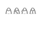
Figure 1: Typical Feynman diagrams contributing to $\zeta_{2}^{0}$, $\zeta_{m}^{0}$, $\zeta_{3}^{0}$, $\tilde{\zeta}_{3}^{0}$, and $\tilde{\zeta}_{1}^{0}$.

The phenomenological implications of Eqs. (4) and (11) are illustrated in Fig. 2. For consistency, $(n+1)$-loop evolution must be accompanied by $n$-loop matching. Figure 2(a) shows how $\alpha_{s}^{(5)}(M_{Z})$, consistently evaluated from $\alpha_{s}^{(4)}(M_{\tau})=0.36$ to a given order, depends on the scale $\mu^{(5)}$, measured in units of the bottom-quark pole mass $M_{b}=4.7$ GeV, where the bottom-quark threshold is crossed. In Fig. 2(b), the analogous study is performed for $m_{c}^{(5)}(M_{Z})$ calculated from $\mu_{c}=m_{c}^{(4)}(\mu_{c})=1.2$ GeV using $\alpha_{s}^{(5)}(M_{Z})=0.118$. As expected, the dependence on the unphysical scale $\mu^{(5)}$ is gradually getting weaker as we go to higher orders.

Figure 2: $\mu^{(5)}$ dependence of (a) $\alpha_{s}^{(5)}(M_{Z})$ calculated from $\alpha_{s}^{(4)}(M_{\tau})=0.36$ and (b) $m_{c}^{(5)}(M_{Z})$ calculated from $\mu_{c}=m_{c}^{(4)}(\mu_{c})=1.2$ GeV and $\alpha_{s}^{(5)}(M_{Z})=0.118$ with evolution at one (dotted), two (dashed), three (dot-dashed), and four (solid) loops and appropriate matching.

3 Effective Lagrangians and Low-Energy Theorems

An interesting and perhaps even surprising aspect of $\zeta_{g}$ and $\zeta_{m}$ is that they carry the full information about the virtual $h$-quark effects on the couplings of a CP-even Higgs boson $H$ to gluons and $q$ quarks, respectively. To reveal this connection, starting from the bare Yukawa Lagrangian of the full theory,

$${\cal L}_{\rm Yuk}=-\frac{H^{0}}{v^{0}}\left(\sum_{q=1}^{n_{l}}m_{q}^{0}\bar{\psi}_{q}^{0}\psi_{q}^{0}+m_{h}^{0}\bar{\psi}_{h}^{0}\psi_{h}^{0}\right),$$ (12)

where $v$ is the Higgs vacuum expectation value, one integrates out the $h$ quark by taking the limit $m_{h}^{0}\to\infty$ and so derives the effective Lagrangian,

$${\cal L}_{\rm Yuk}^{\prime}=-\frac{H^{0}}{v^{0}}\sum_{i=1}^{5}C_{i}^{0}{\cal O}_{i}^{\prime}=-2^{1/4}G_{F}^{1/2}H\sum_{i=1}^{5}C_{i}[{\cal O}_{i}],$$ (13)

which is spanned by a natural basis of composite scalar operators with mass dimension four.$\!{}^{{\bf?}}$ The operators,

$${\cal O}_{1}^{\prime} = \left(G_{\mu\nu}^{0\prime,a}\right)^{2},\qquad{\cal O}_{2}^{\prime}=\sum_{q=1}^{n_{l}}m_{q}^{0\prime}\bar{\psi}_{q}^{0\prime}\psi_{q}^{0\prime},\qquad{\cal O}_{3}^{\prime}=\sum_{q=1}^{n_{l}}\bar{\psi}_{q}^{0\prime}\left(i\not\!\!D^{0\prime}-m_{q}^{0\prime}\right)\psi_{q}^{0\prime},$$

$${\cal O}_{4}^{\prime} = G_{\nu}^{0\prime,a}\left(\nabla^{ab}_{\mu}G^{0\prime,b\mu\nu}+g_{s}^{0\prime}\sum_{q=1}^{n_{l}}\bar{\psi}_{q}^{0\prime}T^{a}\gamma^{\nu}\psi_{q}^{0\prime}\right)-\partial_{\mu}\bar{c}^{0\prime,a}\partial^{\mu}c^{0\prime,a},$$

$${\cal O}_{5}^{\prime} = (\nabla^{ab}_{\mu}\partial^{\mu}\bar{c}^{0\prime,b})c^{0\prime,a},$$ (14)

are only constructed from light degrees of freedom, while all residual dependence on the $h$ quark resides in the Wilson coefficients $C_{i}^{0}$.

The derivation of $C_{i}^{0}$ proceeds similarly to Eq. (9). Considering appropriate one-particle-irreducible Green functions which contain a zero-momentum insertion of ${\cal O}_{h}=m_{h}^{0}\bar{\psi}_{h}^{0}\psi_{h}^{0}$ in the limit $m_{h}^{0}\to\infty$, one finds$\!{}^{{\bf?}}$

$$\zeta_{3}^{0}(-4C_{1}^{0}+2C_{4}^{0})=-\frac{1}{2}\partial_{h}^{0}\Pi_{G}^{0h}(0),\ \zeta_{m}^{0}\zeta_{2}^{0}(C_{2}^{0}-C_{3}^{0})=1-\Sigma_{S}^{0h}(0)-\frac{1}{2}\partial_{h}^{0}\Sigma_{S}^{0h}(0),$$

$$\zeta_{2}^{0}C_{3}^{0}=-\frac{1}{2}\partial_{h}^{0}\Sigma_{V}^{0h}(0),\ \tilde{\zeta}_{3}^{0}(C_{4}^{0}+C_{5}^{0})=\frac{1}{2}\partial_{h}^{0}\Pi_{c}^{0h}(0),\ \tilde{\zeta}_{1}^{0}C_{5}^{0}=\frac{1}{2}\partial_{h}^{0}\Gamma_{G\bar{c}c}^{0h}(0,0),$$ (15)

with $\partial_{h}^{0}=(m_{h}^{02}\partial/\partial m_{h}^{02})$, which may be solved for $C_{i}^{0}$. Only ${\cal O}_{1}^{\prime}$ and ${\cal O}_{2}^{\prime}$ contribute to physical observables. They mix under renormalization as$\!{}^{{\bf?}}$

$$\left[{\cal O}_{1}^{\prime}\right]=\left[1+2\left(\frac{\alpha_{s}^{\prime}\partial}{\partial\alpha_{s}^{\prime}}\ln Z_{g}^{\prime}\right)\right]{\cal O}_{1}^{\prime}-4\left(\frac{\alpha_{s}^{\prime}\partial}{\partial\alpha_{s}^{\prime}}\ln Z_{m}^{\prime}\right){\cal O}_{2}^{\prime},\qquad\left[{\cal O}_{2}^{\prime}\right]={\cal O}_{2}^{\prime},$$ (16)

where the brackets denote the renormalized counterparts. $C_{1}$ and $C_{2}$ are accordingly determined from the second equation in Eq. (13). They are diagrammatically calculated through three loops.$\!{}^{{\bf?}}$ Inserting Eqs. (8) and (9) into Eqs. (15), one obtains the low-energy theorems$\!{}^{{\bf?}}$

$$C_{1}=-\frac{1}{2}\,\frac{\partial\ln\zeta_{g}^{2}}{\partial\ln m_{h}^{2}},\qquad C_{2}=1+2\frac{\partial\ln\zeta_{m}}{\partial\ln m_{h}^{2}},$$ (17)

which are valid to all orders in $\alpha_{s}$. Fully exploiting the present knowledge of Eq. (4),$\!{}^{{\bf?}}$ one may construct the four-loop terms of $\zeta_{g}$ and $\zeta_{m}$ involving $\ln m_{h}^{2}$ and so obtain $C_{1}$ and $C_{2}$ from Eq. (17) to one order beyond the diagrammatic calculation. The expansions in $a=\alpha_{s}^{(n_{f})}(\mu_{h})/\pi$ read$\!{}^{{\bf?}}$

$$C_{1} = -\frac{a}{12}[1+2.7500\,a+(9.7951-0.6979\,n_{l})a^{2}$$

$${}+(49.1827-7.7743\,n_{l}-0.2207\,n_{l}^{2})a^{3}],$$

$$C_{2} = 1+0.2778a^{2}+(2.2434+0.2454\,n_{l})a^{3}$$ (18)

$${}+(2.1800+0.3096\,n_{l}-0.0100\,n_{l}^{2})a^{4}.$$

Having established ${\cal L}_{\rm yuk}^{\prime}$, we are able to make higher-order predictions for the QCD interactions of a light $H$ boson by just computing massless diagrams. For instance, the $H\to gg$ partial decay width at three loops is found to be$\!{}^{{\bf?}}$

$$\Gamma(H\to gg)=\frac{G_{F}M_{H}^{3}}{36\pi\sqrt{2}}a^{\prime 2}\left[1+17.917\,a^{\prime}+a^{\prime 2}\left(156.808-5.708\,\ln\frac{m_{t}^{2}}{M_{H}^{2}}\right)\right],$$ (19)

where $a^{\prime}=\alpha_{s}^{(5)}(M_{H})/\pi$. The three-loop ${\cal O}(\alpha_{s}^{2}G_{F}m_{t}^{2})$ corrections to $\Gamma(H\to q\bar{q})$, with $q=u,d,s,c,b$, may also be obtained from Eq. (13).$\!{}^{{\bf?}}$ Analogously, the QCD interactions of a CP-odd Higgs boson $A$ may be described by an effective Lagrangian involving composite pseudoscalar operators with mass dimension four.$\!{}^{{\bf?}}$ The resulting counterpart of Eq. (19) is found to be$\!{}^{{\bf?}}$

$$\Gamma(A\to gg)=\frac{G_{F}M_{A}^{3}}{16\pi\sqrt{2}}a^{\prime 2}\left[1+18.417\,a^{\prime}+a^{\prime 2}\left(171.544-5\ln\frac{m_{t}^{2}}{M_{A}^{2}}\right)\right],$$ (20)

where $a^{\prime}=\alpha_{s}^{(5)}(M_{A})/\pi$. As a by-product of this analysis,$\!{}^{{\bf?}}$ the Adler-Bardeen nonrenormalization theorem,$\!{}^{{\bf?}}$ which states that the anomaly of the axial-vector current is not renormalized in QCD, is verified through three loops by an explicit diagrammatic calculation.

4 Comparison with Scale Optimization Procedures

It is interesting to compare the exact values of the ${\cal O}(\alpha_{s}^{2})$ corrections in Eqs. (19) and (20) with the estimates one may derive from the knowledge of the ${\cal O}(\alpha_{s})$ correction through the application of well-known scale optimization procedures, based on Grunberg’s concept of fastest apparent convergence (FAC), Stevenson’s principle of minimal sensitivity (PMS), and the proposal by Brodsky, Lepage, and Mackenzie (BLM) to resum the leading light-quark contribution to the renormalization of the strong coupling constant.$\!{}^{{\bf?}}$ The resulting estimates are listed in Table 1. We observe that the sign and the order of magnitude is correctly predicted in all cases.

Table 1: Scale optimization estimates for the ${\cal O}(\alpha_{s}^{2})$ coefficients in Eqs. (19) and (20).

	FAC	PMS	BLM
$H\to gg$	263.3	263.9	242.5
$A\to gg$	277.6	278.1	252.5

5 Summary

A consistent $\overline{\mbox{MS}}$ description of $\alpha_{s}(\mu)$ and $m_{q}(\mu)$ with $\mu$ evolution through four loops and threshold matching through three loops is now available. Effective Lagrangians and low-energy theorems are useful tools to treat the hadronic decays of light CP-even and CP-odd Higgs bosons through three loops. The sign and the order of magnitude of the resulting three-loop corrections are correctly predicted by scale optimization procedures.

References

References

- [1] C.G. Bollini and J.J. Giambiagi, Phys. Lett. 40 B, 566 (1972); G. ’t Hooft and M. Veltman, Nucl. Phys. B 44, 189 (1972).
- [2] G. ’t Hooft, Nucl. Phys. B 61, 455 (1973).
- [3] W.A. Bardeen, A.J. Buras, D.W. Duke, and T. Muta, Phys. Rev. D 18, 3998 (1978).
- [4] J.A.M. Vermaseren, S.A. Larin, and T. van Ritbergen, Phys. Lett. B 400, 379 (1997); 405, 327 (1997); K.G. Chetyrkin, Phys. Lett. B 404, 161 (1997).
- [5] K. Symanzik, Commun. math. Phys. 34, 7 (1973); T. Appelquist und J. Carazzone, Phys. Rev. D 11, 2856 (1975).
- [6] K.G. Chetyrkin, B.A. Kniehl, and M. Steinhauser, Phys. Rev. Lett. 79, 2184 (1997).
- [7] P. Nogueira, J. Comput. Phys. 105, 279 (1993).
- [8] M. Steinhauser, Ph.D. thesis, Karlsruhe University (Shaker Verlag, Aachen, 1996); in these proceedings.
- [9] W. Bernreuther and W. Wetzel, Nucl. Phys. B 197, 228 (1982); 513, 758(E) (1998); W. Bernreuther, Ann. Phys. 151, 127 (1983); Z. Phys. C 20, 331 (1983); 29, 245 (1985); S.A. Larin, T. van Ritbergen, and J.A.M. Vermaseren, Nucl. Phys. B 438, 278 (1995).
- [10] K.G. Chetyrkin, B.A. Kniehl, and M. Steinhauser, Nucl. Phys. B 510, 61 (1998).
- [11] T. Inami, T. Kubota, and Y. Okada, Z. Phys. C 18, 69 (1983); V.P. Spiridonov, INR Report P–0378 (1984).
- [12] K.G. Chetyrkin, B.A. Kniehl, and M. Steinhauser, Phys. Rev. Lett. 79, 353 (1997).
- [13] K.G. Chetyrkin, B.A. Kniehl, and M. Steinhauser, Phys. Rev. Lett. 78, 594 (1997); Nucl. Phys. B 490, 19 (1997).
- [14] K.G. Chetyrkin, B.A. Kniehl, M. Steinhauser, and W.A. Bardeen, Nucl. Phys. B 535, 3 (1998).
- [15] S.L. Adler and W.A. Bardeen, Phys. Rev. 182, 1517 (1969).
- [16] G. Grunberg, Phys. Lett. 95 B, 70 (1980); P.M. Stevenson, Phys. Rev. D 23, 2916 (1981); S.J. Brodsky, G.P. Lepage and P.B. Mackenzie, Phys. Rev. D 28, 228 (1983).