Some experiments on LEAR obtained unusual behavior of the $p\bar{p}$ interaction near the threshold. The experiments on $p\bar{p}$ forvard scattering detected zeros and big variation of $\rho$ and at the same time a smooth rising of ${\sigma}_{tot}$ with lowing energy. Many models has difficulties in explanating this fact. In the PS170 experiment with a good statistical accuracy the unexpected behavior of the proton electromagnetic form factor was found. All these experiments can be considered as an indication for the existence of a low lying $p\bar{p}$ bound state ’baryonium’. This statement coincides with that made for interpretation of the energy dependence of the total cross-section $e^{+}e^{-}\to hadrons$ in FENICE. There is a model (based on analyticity) which explained aforementioned experiments and the fact that this ’baryonium’ is not seen in the OBELIX $p\bar{p}$ annihilation cross-section. Thus LEAR experiments and FENICE one are consistent near $p\bar{p}$ threshold and compatible with the existence of ’baryonium’.
PACS:13.40.Fn—Electomagnetic form factor; electric and magnetic moments.
    14.20—Baryons and baryons resonans(including antiparticles).

1 The database and previous knowledge

The experiment on LEAR which is a part of the CERN antiproton complex gives a rich information about low energy antiproton physics. The experiments (PS172, PS173) [1, 2] on $p\bar{p}$ scattering give the data on $d\sigma/d\Omega$, $\sigma_{tot}$ and $\rho$. To search for bound state cross section measurements are the most straightforward experiments to perform. The analysis of $d\sigma/d\Omega$ gives an indication of the bound states near $p\bar{p}$ threshold [3]. Some of them are consistent with the strong interaction shifts and width of protonium [4]. A resonance (a bound state having a mass bigger the $p\bar{p}$ threshold) may be seen as a bump in $\sigma_{tot}$. But the measurements of the $p\bar{p}$ total cross section above 180 MeV/c indicate its smoothly varying behaviour [2]. The most remarkable result in $p\bar{p}$ elastic scattering has appeared in the data on real-to-imaginary ratio of the forward scattering amplitude $\rho$ which at LEAR was measured down to 180 MeV/c [2]. For the range $350<p_{l}<700~{}MeV/C$ the behaviour of $\rho$ can be explained by insertion of a pole below threshold in the dispersion relation analysis [5]. But LEAR measurements [2, 6] below 350 MeV/c indicate that the $\rho$ is turning upward again. The reason for this unusual behaviour is not yet clear. It might be caused by a $p\bar{p}$ bound state [7] but not by an $n\bar{n}$ threshold [8]. Experimental the $\rho$ was always determined from elastic differential cross section in the Coulomb-nuclear interference region. The method used to extract $\rho$ from such data sometimes has been criticized [9]. But at high energies the method is consistent with the predictions of dispersion relations. So $\rho$ from [2, 6] will be considered below as reliable.
The results of experiment PS–170 on the study of annihilation $p\overline{p}\rightarrow e\overline{e}$ at low energies [10] have no adequate interpretation till the present day. They resulted in an unexpected behaviour of the proton electromagnetic form factor near the $p\overline{p}$– threshold in the time–like region, where $s<4.2~{}GeV^{2}$. The data on
$\mid G\mid=\mid G_{m,p}\mid=\mid G_{e,p}\mid$ point to a large negative derivative at the threshold that rapidly grows to zero or even to positive values at $s\sim$ $4~{}GeV^{2}$. The magnitude of the derivative at the threshold is determined by the threshold value $\mid G\mid=0.53\pm 0.05$. One of the early values, $\mid G\mid=0.51\pm 0.08$, does not contradict the results of ref. [10]. It was obtained [11] from the ratio of frequencies of $p\overline{p}$ annihilations at rest into $e\bar{e}$ and $\pi^{+}\pi^{-}$ pairs in liquid hydrogen. The determination of $\mid G\mid$ at the threshold is a complicated problem since one should simultaneously consider the Coulomb and strong interactions in the $p\overline{p}$–system and requires some approximations. These approximations have been analysed in ref. [12] where a new scheme is proposed for the determination of $\mid G\mid$. This scheme gave the value $\mid G\mid=1.1$ that confirms the results of ref. [10]. Quite recently, a new attempt has been undertaken for determining $\mid G\mid$ at the threshold [13]. Combining the data on widths of $p\overline{p}$–atoms obtained in the synchrotron trap with the results on the low–energy annihilation cross section in $p\overline{p}$–system, the authors concluded that $\mid G\mid=0.39$ or even $\mid G\mid=0.3$. This allows us to infer that there is no abrupt change of $\mid G\mid$ at the threshold. Thus, the authors of [12,13] propose a new view on the method of calculating $\mid G\mid$ at the threshold from experimental data.
Let us now proceed to works that suggest the interpretation of the results of the experiment [10]. In ref. [14] an attempt is made to consider the interaction in the final state. The basic result is the formula $G=ce^{i\delta}$, where $c$ is a slow variable function of $q^{2}$ at the threshold ($q$ is the momentum in c.m.s. of the $p\overline{p}$–system) and $\delta$ is the $N\overline{N}$ scattering phase. Since the phase $\delta$ is complex at the threshold, we have

$$\mid G\mid=\mid c\mid\cdot\mid 1-q\cdot\mbox{Im a}\mid~{},$$ (1)

where a is the complex scattering length. Owing to $\mid G\mid$ being linear in $q$, the quantity $d\mid G\mid/ds$ is infinite at the threshold. Analysis of the first four points from [10] with respect to the $\chi^{2}$–criterion gives the values: $\mid c\mid=0.53\pm 0.02\>,\>\mbox{ Im a}=0.62\pm 0.08\>fm,\>\chi^{2}=0.07$. The authors of [14] employ the values:$\mid c\mid=0.52,\mbox{Im a}\cong 0.8\>fm$; they identify $\mbox{Im}a$ with the quantity $\mbox{Im a}(^{3}S_{1})$ computed from the experiment [15]. The description is qualitative since $\chi^{2}\sim 10$. The authors of [16] assert that a good description of all known data on nucleon electromagnetic form factors, including the data of [10], is obtained on the basis of a new formulation of the vector–dominance model (VDM) and its subsequent unitarization. In what follows, we will use different models of that type, therefore we consider them in detail. They are based on the expressions for the Dirac and Pauli nucleon form factors in VDM:

$$F_{N}(s)=\sum_{v}\frac{f_{v,NN}}{f_{v}}\frac{m^{2}_{v}}{m^{2}_{v}-s},$$ (2)

where $m_{v}$ is the mass of a vector meson, $f_{vNN}$ is the coupling constant of a vector meson with a nucleon, $f_{v}$ is the universal constant in the so–called identity of current and field. Imposing constraints on the parameters of formula (2), one can easily find the experimental value $F_{N}(s=0)$ and the asymptotics following from the quark counting rules [17] that coincides with the QCD–asymptotics within the logarithmic accuracy. Then, the model is unitarized with the help of a uniformizing variable. As a result, vector mesons acquire widths, and the form factors can be calculated for all $s$. So, all experimental data can be described both in the space–like ($s<0$) and time–like ($s>0$) regions. Satisfactory description of more than three hundred values of $\mid F_{N}\mid$ requires about ten free parameters in the formula (2). Besides, this approach allows a model–dependent reproduction of the form of $\mbox{Im}F_{N}$, $\mbox{Re}F_{N}$ in the whole time–like region. This fact will be used below. Results of the analysis according to this scheme are presented in ref. [16]. The data of the experiment PS–170 are explained by including the third radial excitation $\rho(770)$ with the mass $\sqrt{s}=2.15~{}GeV$ into formula (2) and are plotted in Fig.1.

2 Formulation of the analytical model

It is easy to see that the nucleon form factor, according to formula (2), has the following imaginary part

$$\mbox{ImF}_{N}=\pi\sum_{v}m_{v}^{2}\frac{f_{vNN}}{f_{\rho}}\delta(s-m_{v}^{2}).$$ (3)

Formula (3) is an approximate expression obtained from the unitarity condition which allows one to reproduce equation (2) with the use of dispersion relations for $F_{N}$. We write the starting expression for the unitarity condition as follows:

$$\mbox{Im}<o\mid j_{\mu}\mid N\bar{N}>=\sum_{n}<o\mid j_{\mu}\mid n><n\mid T^{+}|N\bar{N}>,$$ (4)

where $j_{\mu}$ is the electromagnetic current of a nucleon $N$, and $|n>$ is the complete set of admissible intermediate states. In our case, it is of the form

$$|n>=|2\pi>,\>|3\pi>,...,|K\bar{K}>,\>|N,\bar{N}>.$$ (5)

Frazer and Fulco [18] were the first who computed the contribution of the two–pion state and predicted the $\rho$–meson on the basis of data on $F_{N}$. By choosing different terms in the sequence (5), one can obtain many models of the type (2). Earlier, the model of ref.[19] was used in [20] and the contribution of an $N\overline{N}$ intermediate state was calculated. This contribution is important for two reasons. First its consideration results in a new branch point in formula (2), the threshold of the reaction $N\overline{N}$ situated on the lower edge of the energy region studied in ref.[10]. Second bound states or resonances in $N\overline{N}$ –system near the threshold will influence the behaviour of $F_{N}(s)$ in the nonobservable region below the $N\overline{N}$–threshold and in the observable region above the $N\overline{N}$–threshold investigated in ref.[10]. It is clear that the state $|N\overline{N}>$ appears on the background of the sum of other states of the series (5) and the result is model–dependent. Therefore, it is important to study the degree of that dependence by considering another model differing from the one used in [20] for $F_{N}(s)$ as a background for the state $|N\overline{N}>$.
We will take the model of ref.[21] formulated in terms of the Sachs form factors $G$ measured experimentally. The model is based on the formulae

$$G_{m,p}(s)=\sum_{k=1}^{3}\frac{\epsilon_{k}(s)}{s-a_{k}-\gamma_{k}\sqrt{s_{k}-s}}\>,\quad G_{e,p}(s)=\sum_{k=1}^{3}\frac{\beta_{k}(s)}{s-a_{k}-\gamma_{k}\sqrt{s_{k}-s}}\>,$$ (6)

$$\mbox{where}\quad\epsilon_{k}(s)=\frac{\epsilon_{k}^{1}+\epsilon_{k}^{0}s}{s-a_{k}-\gamma_{k}\sqrt{s_{k}-s}}\>,\quad\beta_{k}(s)=\frac{\beta_{k}^{1}+\beta_{k}^{0}s}{s-a_{k}-\gamma_{k}\sqrt{s_{k}-s}}\cdot$$ (7)

The energy behaviour of electromagnetic form factors is explained with the use of three resonances:$\rho$, $\omega$, $\varphi$ specified by indices $k=1,2,3$ in formula (6). The masses, widths and thresholds $a_{k},\gamma_{k},s_{k}$ are taken from experiment. The model parameters are the coupling constants

$$(\beta_{1}^{1}+\epsilon_{1}^{0}s)f_{1}(s)=g_{\gamma\rho}(s)g_{\rho NN}(s),$$

$$(\beta_{2}^{1}+\epsilon_{2}^{0}s)f_{2}(s)=g_{\gamma\omega}(s)g_{\omega NN}(s),$$

$$(\beta_{3}^{1}+\epsilon_{3}^{0}s)f_{3}(s)=g_{\gamma\phi}(s)g_{\phi NN}(s)\>,$$

where

$$f_{k}(s)=\frac{1}{s-a_{k}-\gamma_{k}\sqrt{s_{k}-s}}\cdot$$ (8)

This unusual form of the constants is chosen by analogy with the index of refraction in optics. They are not only energy–dependent, but also contain a complex component when $s>s_{k}$. The coupling constants are chosen so as to be consistent with the known experimental data at $s=0$. Then, we are left with two free parameters $\epsilon_{2}^{0}$ and $\epsilon_{3}^{0}$ to be defined from the conditions required at $s\rightarrow\infty$. The $SU(3)$ symmetry should hold on the asymptotics identically. This condition seems to be the weakest one since it can be changed by including new vector mesons into consideration. Therefore, the parameters $\epsilon_{2}^{0}$ and $\epsilon_{3}^{0}$ are determined according to the $\chi^{2}$ criterion on the basis of experimental points $|G_{p}|$ cited in refs. [22]. An interesting feature of the model [21] is that it correctly describes the ratio $|G_{p}|/|G_{n}|$ above the $p\bar{p}$–threshold. More exactly, it reproduces the experimental value $|G_{n}(s=4~{}GeV^{2})|=0.42\pm 0.06$ (see [23]). The model result for $|G_{p}|$ is drawn in Fig.2. and $\epsilon^{0}_{2}=-3.41,\epsilon^{0}_{3}=3.23,\chi^{2}=10.1$.
The influence of the $|N\bar{N}>$   contribution to the unitarity condition (4) on $|G|$ is computed in the same way as in refs. [20, 24]. We construct the analytic model for the forward elastic scattering amplitude $T$ in terms of the uniformizing variable

$$z=\sqrt{\frac{4(s-\alpha)}{s(4-\alpha)}}-\sqrt{\frac{\alpha(s-4)}{s(4-\alpha)}},$$ (9)

where $s$ is the conventional Mandelstam variable equal to the square of the total energy of a $p\bar{p}$–system in the c.m.s. in units $M_{p}$. The variable $z$ contains branch points at $s=0;4$ corresponding to the reaction threshold of elastic $pp$ and $p\bar{p}$–scattering and an effective branch point at $s=\alpha$ corresponding to the nonobservable region for the elastic $p\bar{p}$– scattering. The threshold of process $p\bar{p}\rightarrow p\bar{p}$ is mapped into points $z=\pm 1$ on the $z$–plane; whereas the infinit $s$–plane point, into points $\pm z_{1},\>\pm 1/z_{1}$, where $z_{1}=\sqrt{\frac{2-\sqrt{\alpha}}{2+\sqrt{\alpha}}}$. Disposition of all the four sheets of the Riemann surface of the function $z(s)$ is drawn in Fig.3 for $\alpha=1.44$. In ref. [24] it is shown that the experimental data on $\rho=\mbox{Re}T/\mbox{ImT}$ and $\sigma_{tot}$ can be well described provided that the $p\bar{p}$–system possesses a quasinuclear bound state with the binding energy $E=(1.88\pm 0.05)~{}MeV$ and width $\Gamma=(1.6\pm 0.1)~{}MeV$. The scattering amplitude was taken in the form

$$T=T_{b}+\frac{c_{\rho}}{z-(z_{\rho})_{1}}-\frac{c_{\rho}}{z-(z_{\rho})_{2}},$$ (10)

where $T_{b}(s)$ is a polynomial in $z$, $(z_{\rho})_{1,2}=1\mp\gamma\pm i\delta$ and $\alpha=1.44,10^{2}\gamma=-0.54\pm 0.02,10^{2}\delta=2.6\pm 0.08$. The pole terms represent the contribution of the quasinuclear state; whereas the polynomial determines the contribution of a nonresonance background of S,P and D–waves. Special attention was paid to the threshold value of the $T$ amplitude which is complex [24]. The amplitude (10) well describes the experimental data up to $4.4~{}GeV^{2}$ in terms of the variable $s$. It is valid in the vicinity of $z=1$ and has two poles in distinction to the usual quantum mechanical amplitude. Appearence of the two poles in the variable z inctead of the one pole in the variable $q$ in the scattering amplitude $T$ is a consequence of choosing z as uniformazing variable. Another important feature of the formula (10) is the form of the pole term contribution to Im T and Re T. The bound state (pole) contribution to the $\mbox{ImT}(p_{l}=80~{}MeV/c)$ is about 10% of the total value $\mbox{Im T}_{p\bar{p}}$. On the other hand, the bound state contribution to the ReT is larger then the background one and ensure the correct value $\rho$ (see Fig. 4,5). Near the $p\bar{p}$–threshold the pole contribution to the unitarity condition (4) becomes dominant, and thus, we will restrict ourselves to the pole approximation. Quantum numbers of this state are unknown. A detailed scheme of calculation corresponds to the scheme by Frazer and Fulco [18] for the contribution of different partial waves to $\mbox{Im}F_{N}$. In our case, it gives that these states are either ${}^{3}S_{1}$ or ${}^{3}D_{1}$. Then, the unitarity condition (4) is reduced to the Riemann boundary–value problem [25] that can be solved (see Appendix). Inside the ring containing the unit circle (Fig.3) the solution is of the form

$$G_{pol}=\frac{c(z)}{\prod_{i=1}^{2}(z-(z_{\rho})_{i})(z+(z_{\rho}^{*})_{i})},$$ (11)

where $c(z)$ is an entire function within which the solution is determined. Setting $c(z)=c_{1}(z)\cdot(z^{2}-z_{1}^{2})(1-z^{2}z_{1}^{2})/(1-z_{1}^{2})^{2}$, we can ensure the asymptotic behaviour of $G_{pol}$ at infinity. Taking advantage of $c_{1}(z)$ being arbitrary, we assume the solution to be of the form

$$G_{pol}(z)\frac{(1-z_{1}^{2})^{2}}{(z^{2}-z_{1}^{2})(z^{2}z_{1}^{2}-1)}=$$ (12)

$$A_{1}\biggl{\{}\Bigl{(}\frac{1}{z-(z_{\rho})_{1}}-\frac{1}{z-(z_{\rho})_{2}}\Bigr{)}-\Bigl{(}\frac{1}{z+(z_{\rho}^{*})_{1}}-\frac{1}{z+(z_{\rho}^{*})_{2}}\Bigr{)}\biggr{\}}+$$

$$+A_{2}\biggl{\{}\Bigl{(}\frac{1}{z-(z_{\rho})_{1}}+\frac{1}{z-(z_{\rho})_{2}}\Bigr{)}-\Bigl{(}\frac{1}{z+(z_{\rho}^{*})_{1}}+\frac{1}{z+(z+(z_{\rho}^{*})_{2}}\Bigr{)}\biggr{\}}.$$

Around the $p\bar{p}$–threshold the equalities $\mid G_{e,p}\mid=\mid G_{m,p}\mid=\mid G\mid$ hold valid and, under this assumption, the experiment in [10] was analysed. Therefore, we put

$$G_{e,p}+G_{m,p}=2G_{w},$$ (13)

where the functions $G_{e(m),p}$ are given by formulae (6). Considering the contribution of the $|N\bar{N}>$–state to the unitarity condition (4), we obtain for the proton electromagnetic form factor $G$:

$$G=G_{w}+G_{pol}.$$ (14)

We shall assume the position of poles to be known from ref. [24]; then, the form factor $G$ depends on two free parameters $A_{1},A_{2}$. The behaviour of $G_{pol}$ on the upper edge of the cut $[\alpha,\infty)$ around the $N\bar{N}$–threshold is determined by the poles $(z_{\rho})_{1}$ and $(z_{\rho})_{2}$; whereas on the lower edge, by the poles $(z_{\rho}^{*})_{1}$ and $(z_{\rho}^{*})_{2}$. If we calculate the common denominator for the contributions of the poles $(z_{\rho})_{1}$ and $(z_{\rho})_{2}$ in the formula (12), the energy factor $(z-1)$ will arise in front of the parameter $A_{2}$; whereas a constant, in front of the parameter $A_{1}$. This allows us to draw analogy between the parameter $A_{1}$ and $\epsilon^{1}_{k},\beta^{1}_{k}$ as well as between $A_{2}$ and $\epsilon^{0}_{k},\beta^{0}_{k}$ in formula (7). The expression for $G_{pol}$ (11) follows from the unitarity condition and analytic properties of the proton form factor and $N\bar{N}$–scattering amplitude. Therefore, formulae (6) are substantiated, irrespective of the above mentioned analogy with optics. The result of the analysis (Fig. 4) according eq. (12) is presented in the table 1 and parameters are equal: $\alpha=0.23\pm 0.04$, $\epsilon^{o}_{2}=2.97\pm 0.03$, $\epsilon^{o}_{3}=3.23$, $10^{2}A_{1}=0$, $10^{2}A_{2}=1.2\pm 0.01$.

3 Discussion of the results

The parameters $A_{1}$ and $A_{2}$ representing the coupling constants of a quasinuclear bound state are sensitive to the background shape in formula (14) as follows from comparision of this fit and the fit of ref.[20] ($A_{1}\not=0$ in ref.[20]). The magnitude of the background is determined by the parameters $\epsilon^{0}_{2}$ and $\epsilon^{0}_{3}$ and is slow changing function in the s interval under investigation. The parameters $A_{1},A_{2},\alpha$ determine the rapid change of $G$ in formula (14). Via separating the parameters into these two groups, we can obtain their statistically reasonable values (table 1). The analysis would be considerably simplified if the experimental values of $s>4M^{2}_{p}$ were known for $\mbox{Im}G$ and $\mbox{Re}G$. Their determination requires polarization experiments whose theoretical study is carried out in ref. [26].
Recently two independent experiments gave new information on the $p\bar{p}$ interaction at low energy. The value of the $p\bar{p}$ annihilation total cross section down to the momenta 43 MeV/c have been measured by OBELIX experiment [27] at LEAR and no resonant behaviour of the cross section was found.The existence of some stracture in the $e\bar{e}\to hadrons$ cross section near the $P\bar{P}$ threshold was indicated in FENICE at ADONE [28]. A combined analysis of these data and the data on the proton form factor provides a good candidate for the quasinucler bound state with the mass $M=1.85\pm 0.01~{}GeV^{2}$ and the width $\Gamma=40\pm 10~{}MeV$. This candidate dosn’t contradict our candidate [20]. Then the question arise why this candidat is not seen in the OBELIX experiment on the $p\bar{p}$ annihilation cross section at very low energy. The first reason for that is the mass of ’baryonium’ which is less then $2M_{p}$. The second is based on our analytical model. In this model $(\sigma_{tot})_{pole}\simeq 0.1~{}\sigma_{tot}$ at low energy (see Fig. 4) but $\sigma_{ann}<\sigma_{tot}$. From these inequalities it is clear why ’baryonium’ is not seen in OBELIX data. On the other hand, in FENICE experiment cross section $e^{+}e^{-}\rightarrow hadrons$ depends not only on ImT but also on ReT for which the pole contribution is large. That is the reason why ’baryonium’ is not seen in OBELIX and seen in FENICE. Thus the results of bouth this experiments are consistent.
Finaly we mention a pure theoretical result; the method of derivation of formula (11) for describing a quasinuclear state can be applied to any vector meson in formula (2). Therefore any vector meson will be characterized not only by the mass and width but also by two parameters like coupling constants. In other words, the effective coupling constants will be energy–dependent, what is assumed in ref. [21] and is reflected in formulae (7).

Appendix

The unitarity condition (4) is an exact equation if use is made of the complete system of admissible intermediate states (5), otherwise it is an approximate equation dependent on the assumptions made. Let us take it in the form

$$\mbox{ImF}=F(e^{i\delta}\sin{\delta})^{*}+\bar{g},$$

where $\delta$ is the $N\bar{N}$–scattering phase with quantum numbers of the pole state unknown yet; $\overline{g}$ is the contribution of all other processes in the same channel. We reduce it to the form

$$F=e^{2i\delta}F^{*}+2ig.$$ (A.1)

The relation (A.1) is valid for $\mbox{Im}s=0$ and $\mbox{Re}s\geq 4M^{2}_{p}$. The function $F$ is analytic in the complex plane $s$ with the cut $[4M^{2}_{p},\infty)$ outside of which $F^{*}(s)=F(s^{*})$. This relation represents a linear inhomogeneous Riemann boundary–value problem for the function $F$. If $e^{2i\delta}$ has a pole near the cut, then in its vicinity we can consider the homogeneous problem

$$F=e^{2i\delta}F^{*}.$$

As it is known [25], the main difficulty in solving it consists in constructing a function analytic in the plane $s$ and coincident on the cut with $e^{2i\delta}$. However, if $e^{2i\delta}$ is taken in the form admitting the analytic continuation onto complex $s$, the problem is reduced to the solution of a functional equation for $F$ in the uniformizing variable $z$. We will represent $e^{2i\delta}$ in the form

$$e^{2i\delta}=\prod_{j}\frac{(z-z_{j}^{*})(z+z_{j})}{(z-z_{j})(z+z_{j}^{*})}.$$

The function $e^{2i\delta}$ is real on the imaginary axis $z$, i.e. on the real axis $s$ when $s<\alpha$. Equation (A.1) is valid on the cut $[4M^{2}_{p},\infty)$ that transforms into the real axis $z=x+iy$ , and $F(s)\rightarrow F(x),\>F^{*}(s)\rightarrow F(-x)$

$$F(x)=\frac{(x-z_{j}^{*})(z+z_{j})}{(x-z_{j})(z+z_{j}^{*})}F(-x),$$

where we took only one pole, without loss of generality. The latter functional equation for $F(x)$ can be written as follows

$$F(x)(x-z_{j})(x+z_{j}^{*})=G(x),$$

$$G(x)=G(-x)$$

and thus $F(z)$ is representable in the form

$$F(z)=\frac{G(z)}{\prod_{j}(z-z_{j})(z+z_{j}^{*})},$$

where $G(z)$ is an entire even function of the variable $z$. The inhomogeneous boundary–value problem (A.1) can be solved in a similar manner and formula (11) can be proved.

Table 1:

$S\>~{}GeV^{2}$	$G_{exp}$	$|G|$	$\chi^{2}_{i}$
3.523	$0.53\pm 0.05$	0.63	3.9
$3.553$	$0.39\pm 0.05$	0.35	0.63
$3.57$	$0.34\pm 0.04$	0.32	0.26
$3.59$	$0.31\pm 0.03$	0.3	0.15
$3.76$	$0.26\pm 0.014$	0.27	0.66
$3.83$	$0.25\pm 0.01$	0.27	1.9
$3.94$	$0.247\pm 0.014$	0.254	0.23
$4.18$	$0.252\pm 0.011$	0.221	8.1

Figure Captions.

Fig. 1. The curve from Fig. $3^{a}$ of ref.[16] on a larger scale. The quality of the fit PS-170 data is very poor.
Fig. 2. Our fit to the old data [22] by $G_{w}$.
Fig. 3. Disposition of four sheets of the Riemann surface of the function z(s)
for $\alpha=1.44$. The threshold $p\bar{p}$ is mapped into points $z=\pm 1$.
Fig. 4. The pole contribution to the $\mbox{ImT}.$
Fig. 5. The pole contribution to the $\rho.$
Fig. 6. Our fit to PS-170 data with account of the pole contribution (eq.(12)).

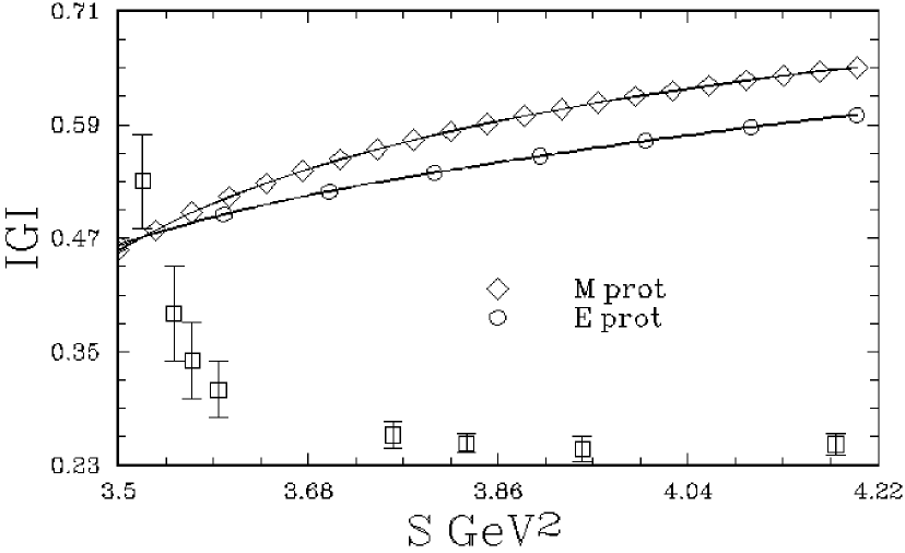
Figure 1:

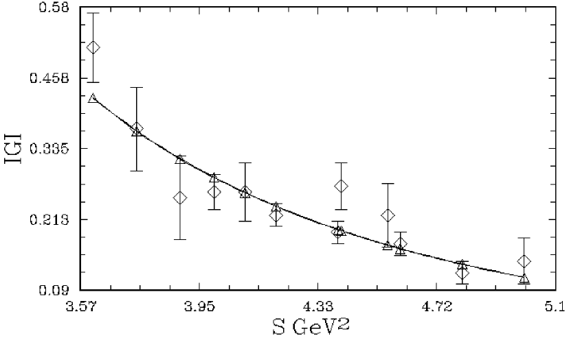
Figure 2:

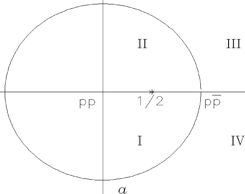
Figure 3:

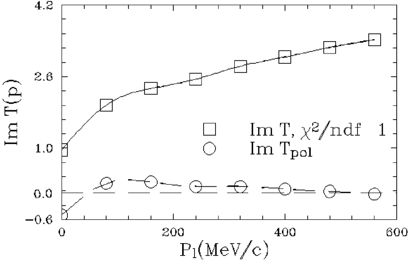
Figure 4:

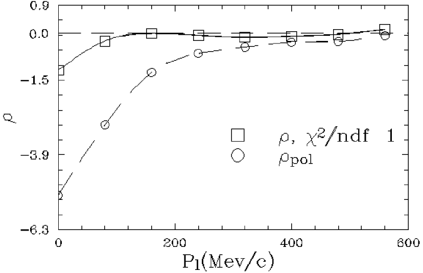
Figure 5:

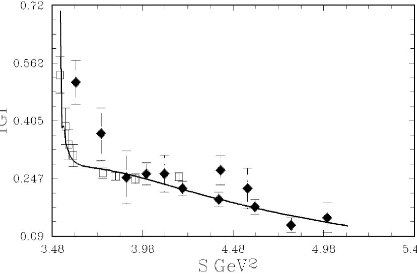
Figure 6:

References

-
[1]
R. A .Kunne, C. I. Beard, R. Birsa, K. Bos, F. Bradamante, D. V. Bugg,
A. S. Clough, S. Dallatorre-Colautti, S. Delgi-Agosti, J. I. Edgington, J. R. Holl, E. Heer,
R. Hess, J. C. Kluyver, C. Lechanoine-Lelae, L. Linssen, A. Martin, T. O. Ninikoski, Y. Onel,
A. Penzo, D. Rapin, J. M. Rieubland, A. Rijllart, P. Schiavon, R. L. Shypit, F. Tessarotto,
A. Villari, P. Wells,
Phys. Lett. B206, 557 (1998); Nucl. Phys. B323, 1 (1989). - [2] W. Brückner, H. Döbbeling, F. Güttner, D. von Harrach, H. Kneis, S. Majewski, M. Nomachi, S. Paul, V. Povh, R. D. Ransome, T. A. Shibata, M. Treichel, Th. Walcher, Phys. Lett. B158, 180 (1985); ibid. B166,113 (1986).
- [3] V. K. Henner, V. A. Meshcheryakov, Zeit. Phys. A345, 215 (1993).
- [4] V. K. Henner, V. A. Meshcheryakov, Yad. Phys. 58, 320 (1995).
- [5] H. Iwasaki, H. Aihara, J. Chiba, H. Fuji, T. Fuji, T. Kamae, K. Nakamura, T. Suiyoshi, Y. Takeda, M. Yamauchi, H. Fukuma, Nucl. Phys. A433, 433 [1985).
- [6] L. Linssen, C. I. Beard, R. Birsa, K. Bos, F. Bradamate, D. V. Bugg, A. S. Clough, S. Dalla Torre-Colzatti, M. Giorgi, J. R. Hall, J. C. Klugver, R. A. Kunne, C. Lechanione-Lelae, A. Martin, Y. Onel, A. Penzo, P. Rapin, P. Schiavon, R. L. Shypit, A. Villari, Nucl. Phys. A469, 726 (1987).
- [7] B. V. Bykovsky, V. A. Meshcheryakov, D. V. Meshcheryakov, Yad. Phys. 55, 1186 (1992).
- [8] J. Mahalanubis, H. J. Pirner, T. A. Shibata, Nucl. Phys. A485, 546 (1988).
- [9] J. J. de Swart, R. Timmermans, in: Proceedings of the Third Biennial Conference on Low Energy Antiproton Physics, Bled, Slovenia, September 1994 (edited by G. Kernel, P. Kriz̆an, M. Mikuz̆), World Scientific,1995 p. 20.
- [10] G. Bardin, G. Burgun, R. Calabrese, G. Capon, R. Carlin, P. Dalpiaz, P. F. Dalpiaz, J. Derre, U. Dosselli, J. Duclos, J. L. Faure, F. Gasparini, M. Huet, C. Kochowski, S. Limentani, E. Luppi, G. Marel, E. Mazzucato, F. Petrucci, M. Posocco, M. Savrie, R. Stroili, L. Tecchio, C. Voci, N. Zekri, Phys.Lett. B255, 149 (1991); B257, 514 (1991).
- [11] G. Bassompierre, G. Binder, P. Dalpiaz, P. F. Dalpiaz, G. Gissinger, S. Jacquey, C. Peroni, M. A. Schneegans and L. Tecchio, Phys. Lett. B68, 477 (1977).
- [12] B. Kerbikov and L. A. Kondratyuk, Z. Phys. A340, 181 (1991).
- [13] B. O. Kerbikov, A. E. Kudryavtsev, Nucl. Phys. A558, 177c (1992).
- [14] O. D. Dalkarov, K. V. Protasov, Sov. J. Nucl. Phys. 50, 1030 (1989); Nucl. Phys. A504, 845 (1989); Phys. Lett.B280, 107 (1992).
- [15] R. Bacher, in: Proc. First Bienual Conf. on Low Energy Antiproton Physics, Stockholm. 2–6 July 1990,(Ed. P. Carlson, A. Kerek, S. Szilagyi), World Sientific, 1991, p. 373
- [16] S. Dubnic̆ka, Z. Dubnic̆kova, P. Striz̆enec, Nuovo Cim. A106, 1253 (1993).
- [17] V. A. Matveev, R. M. Muradyan, A. N. Tavkhelidze,Nuovo Cim. Lett. 7, 719 (1974).
- [18] W. R. Frazer, J. R. Fulco, Phys. Rev. 117, 1603, 1609 (1960).
- [19] S. I. Bilenkaya, S. Dubnic̆ka, Z. Dubnic̆kova and P. Striz̆enec, Nuovo Cim. A105, 1421 (1992).
- [20] G. V. Meshcheryakov, V. A. Meshcherykov, Modern Phys. Lett. A9, 1603 (1994).
- [21] V. Wataghin, Nucl. Phys. B10, 107 (1969).
- [22] S. Dubnic̆ka, Nuovo Cim. A100, 1 (1988).
- [23] E. Luppi, Nucl. Phys., A558, 165c (1993).
- [24] B. V. Bykovsky, V. A. Meshcheryakov, D. V. Meshcheryakov, Yad. Fiz. 53, 257 (1990); Yad. Fiz. 55, 1186 (1992).
- [25] M. Muskhelishvili, Singular Integral Equation, Groningen, 1953.
- [26] S. M. Bilenky, C. Giunti, V. Wataghin, Z. Phys. C59, 475 (1993).
- [27] A. Bertin, M. Bruschi, M. Capponi, B. Cereda, S. De Castro, A. Ferreti, D. Galli, B. Giacobbe, U. Marconi, M. Piccinini, N. Semprini-Cesaro, R. Spighi, S. Vecchi, A. Vezzani, F. Vigotti, M. Villa, A. Vitale, A. Zoccoli, G. Belli, M. Corradini, A. Donzella, E. Lodi-Rizzini, L. Venturelli, A. Zenoni, C. Cicaio, A. Masoni, G. Puddu, C. Serci, P. Temnikov, G. Usai, V. G. Ableev, Y. U. Denisov, O. E. Gorchakov, S. N. Prahov, A. M. Rozhdestvensky, M. G. Sapozhnikov, V. I. Tretyak, M. Poli, P. Gianotti, C. Guaraldo, A. Lanaro, V. Lucherini, F. Nicitiu, C. Petrascu, A. Rosca, C. Cavion, U. Gastaldi, M. Lombardi, L. Vannucci, G. Vedovato, A. Andrigetto, M. Morando, R. A. Ricci, G. Bendiscioli, V. Filippini, A. Fontana, P. Montagna, A. Rotondi, A. Saino, P. Salvini, A. Filippi, F. Balestra, E.Botta, T. Bressani, M. P. Bussa, L. Busso, D. Calvo, P. Cerello, S. Costa, F. D’Isep, L. Fava, A. Feliciello, L. Ferrero, R. Garfagnini, A. Grasso, A. Maggiora, S. Marcello, N. Mirfakhraee, D. Panzieri, D. Parena, E. Rossetto, F. Tosello, G. Zosi, M. Angello, F. Iazzi, B. Minetti, G. Pauli, S. Tessaro, L. Santi, Yad. Fiz. 59, 1430 (1996).
- [28] A. Antonelli, R. Baldini, M. Bertani, M. E. Biagini, V. Bidoli, C. Bini, T. Bressani, R. Calabrese, R. Cardanelli, R. Carlin, C. Csari, L. Cugusi, P. Dalpiaz, G. De Zorzi, A. Feliciello, M. L. Ferrer, P. Ferretti, P. Gauzzi, P. Gianotti, E. Luppi, S. Marcello, A. Masoni, R. Messi, M. Morandin, L. Paoluzi, E. Pasqualucci, G. Pauli, N. Perlotto, F. Petrucci, M. Posocco, G. Puddu, M. Reale, L. Santi, R. Santonico, P. Sartori, M. Savrie, S. Serci, M. Spinetti, S. Tessaro, C. Voci, F. Zuin, in: Proceedings of the Third Biennial Coference on Low-Energy Antiproton Physics (Ed. G. Kernel, P. Kriz̆an, M. Mikuz̆), World Scientific, 1995, p. 87.