Limits on Majorana Neutrinos from Recent Experimental Data

Abstract

We investigate the sensitivity of some weak processes to the simplest extension of the Standard Model with Majorana neutrinos mixing in the leptonic sector. Values for mixing angles and masses compatible with several experimental accelerator data and the most recent neutrinoless double-$\beta$ decay limit were found.

I Introduction

Experimental neutrino physics has regained great interest in the latest years, with many new experiments presently taking data or in preparation for the near future. This is justified because although the Standard Model has been vigorously tested experimentally and seems to be a remarkably successful description of nature, its neutrino sector has yet been poorly scrutinized. We believe that this still mysterious area of particle physics may give us some hint on the physics beyond the Standard Model.

It is a common prejudice in the literature to assume the conservation of the leptonic number and to think about neutrinos as Dirac particles much lighter than any of the charged leptons we know. Nevertheless there are no theoretically compelling reasons why the leptonic number should be a conserved quantity or why neutrinos should not have a mass comparable to the charged fermions. It is clear that only the confrontation of theory with experimental data will eventually clarify the problem of neutrino mass and nature.

Many direct limits on neutrino mass have been obtained by different experimental groups [1] but are not all accepted without controversy [2, 3]. Experiments also have been carried out to try to measure neutrinoless double-$\beta$ decay which, in general, is a process that will not occur unless one has a Majorana neutrino involved as an intermediate particle. Here also experiments have obtained only limits on the so called effective neutrino mass [4]. As a rule experimental analysis are model dependent and cannot be quoted as a general result.

In the hope of contributing to the understanding of neutrinos physics we have accomplished a comprehensive study of the constraints imposed by recent experimental data on lepton decays, pion and kaon leptonic decays as well as by the $Z^{0}$ invisible width measurement performed by the LEP experiments to the simplest model containing Majorana neutrinos.

We will consider a very simple extension of the standard electroweak model which consists in adding to its particle content a right-handed neutrino transforming as a singlet under $\text{SU(2)}_{L}\otimes\text{U(1)}_{Y}$. This will be referred as the Minimal Model with Right-handed Neutrino (MMRN). Next, by allowing it to mix with all the left-handed neutrinos we obtain that there are, at the tree level, two massless neutrinos ($m_{1}$, $m_{2}$) and two massive ones ($m_{P}$, $m_{F}$) [6].

It is interesting to note that this simple extension of the Standard Model imposes a mass hierarchy for neutrinos. The massless neutrinos ($m_{1}$, $m_{2}$) can acquire very small mass by radiative corrections [7, 8]. This seems to be consistent with the recent evaluation of the the number of light neutrino species from big bang nucleosynthesis [9].

The outline of this work is as follows. In Sec. II the model consider is briefly reviewed. In Sec. III we consider the effects of mixing for the decay width of the muon, for the partial leptonic decay widths of the tau, pion and kaon and for the $Z^{0}$ invisible width. These are the quantities that are calculated theoretically. In Sec. IV we compare our theoretical results with recent experimental data and obtain from this comparison allowed regions for mixing angles and masses. In Sec. V we investigate the possibility of further constraining our results with the present best limit from neutrinoless double-$\beta$ decay experiments. Finally, in the last section we establish our conclusions.

II A brief description of the model

In the MMRN the most general form of the neutrino mass term is

$${\cal L}_{\nu}^{M}=-\sum_{\alpha=e,\mu,\tau}a_{\alpha}\overline{{\nu_{\alpha}}}_{L}N_{R}-\frac{1}{2}M\overline{N^{c}_{R}}N_{R}+H.c.$$ (1)

where the left-handed neutrino fields are the usual flavor eigenstates and we have assumed that the charged leptons have already been diagonalized. In this model, there are four physical neutrinos $\nu_{1},\nu_{2},\nu_{P}$ and $\nu_{F}$, the first two are massless ($m_{1}=m_{2}=0$) and the last two are massive Majorana neutrinos with masses

$$m_{P}=\frac{1}{2}(\sqrt{M^{2}+4a^{2}}-M)~{}\text{ and }~{}m_{F}=\frac{1}{2}(\sqrt{M^{2}+4a^{2}}+M),$$ (2)

where $a^{2}=a_{e}^{2}+a_{\mu}^{2}+a_{\tau}^{2}$.

In terms of the physical fields the charged current interactions are

$${\cal L}^{CC}=\frac{g}{\sqrt{2}}\begin{array}[]{cccc}(\overline{\nu_{1}}&\overline{\nu_{2}}&\overline{\nu_{P}}&\overline{\nu_{F}}\end{array})_{L}\gamma^{\mu}\Phi R\left(\begin{array}[]{c}e\\ \mu\\ \tau\\ 0\end{array}\right)_{L}W_{\mu}^{+}+H.c.,$$ (3)

where $\Phi=diag(1,1,i,1)$ and $R$ is the matrix

$$\left(\begin{array}[]{cccc}R_{e1}&R_{\mu 1}&R_{\tau 1}&R_{01}\\ R_{e2}&R_{\mu 2}&R_{\tau 2}&R_{02}\\ R_{eP}&R_{\mu P}&R_{\tau P}&R_{0P}\\ R_{eF}&R_{\mu F}&R_{\tau F}&R_{0F}\\ \end{array}\right)=\left(\begin{array}[]{cccc}c_{\beta}&-s_{\beta}s_{\gamma}&-s_{\beta}c_{\gamma}&0\\ 0&c_{\gamma}&-s_{\gamma}&0\\ c_{\alpha}s_{\beta}&c_{\alpha}c_{\beta}s_{\gamma}&c_{\alpha}c_{\beta}c_{\gamma}&-s_{\alpha}\\ s_{\alpha}s_{\beta}&s_{\alpha}c_{\beta}s_{\gamma}&s_{\alpha}c_{\beta}c_{\gamma}&c_{\alpha}\end{array}\right).$$ (4)

In Eq. (4) $c$ and $s$ denote the cosine and the sine of the respective arguments. The angles $\alpha,\beta$ and $\gamma$ lie in the first quadrant and are related to the mass parameter as follows

$$s_{\alpha}=\sqrt{m_{P}/(m_{P}+m_{F})},$$ (5)

$$s_{\beta}=a_{e}/a,\;c_{\beta}s_{\gamma}=a_{\mu}/a,\;c_{\beta}c_{\gamma}=a_{\tau}/a.$$ (6)

The choice of parameterization is such that for $\alpha=\beta=\gamma=0$ , $\nu_{1}\rightarrow\nu^{\prime}_{e}$, $\nu_{2}\rightarrow\nu^{\prime}_{\mu}$ and $\nu_{P}\rightarrow\nu^{\prime}_{\tau}$.

The neutral current interactions for neutrinos written in the physical basis of MMRN read

$${\cal L}^{NC}=\frac{g}{4\cos\theta_{W}}\left(\begin{array}[]{cccc}\overline{\nu_{1}}&\overline{\nu_{2}}&\overline{\nu_{P}}&\overline{\nu_{F}}\end{array}\right)_{L}\gamma^{\mu}\left(\begin{array}[]{cccc}1&0&0&0\\ 0&1&0&0\\ 0&0&c^{2}_{\alpha}&ic_{\alpha}s_{\alpha}\\ 0&0&-ic_{\alpha}s_{\alpha}&s^{2}_{\alpha}\end{array}\right)\left(\begin{array}[]{c}\nu_{1}\\ \nu_{2}\\ \nu_{P}\\ \nu_{F}\end{array}\right)_{L}Z_{\mu}+H.c.$$ (7)

Notice that there are four independent parameters in MMRN. We will choose them to be the angles $\beta$ and $\gamma$ and the two Majorana masses $m_{P}$ and $m_{F}$. These are the parameters that we will constrain with experimental data.

III Four generation mixing in the leptonic sector

In this section we will present the expressions that will be used in our analysis for muon and tau leptonic decays, pion and kaon leptonic decays and the $Z^{0}$ invisible width. The coupling constant $G$ and the decay constants $F_{\pi}$ and $F_{K}$ used in our theoretical expressions have not the same values of the standard $G_{\mu}$, $f_{\pi}$ and $f_{K}$ given in Ref. [1], this important point will be discussed at the end of this section.

A Lepton decays

We can now write the most general expression for the partial decay width of a lepton $l^{\prime}$ into a lepton $l$ and two neutrinos $\bar{\nu}_{l}\nu_{l^{\prime}}$ in the context of MMRN as

$$\Gamma(l^{\prime}\to l\bar{\nu}_{l}\nu_{l^{\prime}}) = \frac{G^{2}m^{5}_{l^{\prime}}}{192\pi^{3}}{\cal R}^{l^{\prime}}\left\{\left(|R_{l^{\prime}1}|^{2}+|R_{l^{\prime}2}|^{2}\right)\left(|R_{l1}|^{2}+|R_{l2}|^{2}\right)\,\Gamma^{l^{\prime}l}_{11}\right.$$ (8)

$$+ \left.\left(|R_{lP}|^{2}[|R_{l^{\prime}1}|^{2}+|R_{l^{\prime}2}|^{2}]+|R_{l^{\prime}P}|^{2}[|R_{l1}|^{2}+|R_{l2}|^{2}]\right)\,\Gamma^{l^{\prime}l}_{1P}\right.$$ (9)

$$+ \left.\left(|R_{lF}|^{2}[|R_{l^{\prime}1}|^{2}+|R_{l^{\prime}2}|^{2}]+|R_{l^{\prime}F}|^{2}[|R_{l1}|^{2}+|R_{l2}|^{2}]\right)\,\Gamma^{l^{\prime}l}_{1F}\right.$$ (10)

$$+ \left.\left(|R_{lF}|^{2}|R_{l^{\prime}P}|^{2}+|R_{l^{\prime}F}|^{2}|R_{lP}|^{2}\right)\,\overline{\Gamma}^{l^{\prime}l}_{PF}\right.$$ (11)

$$+ \left.|R_{l^{\prime}P}|^{2}|R_{lP}|^{2}\,\overline{\Gamma}^{l^{\prime}l}_{PP}+|R_{l^{\prime}F}|^{2}|R_{lF}|^{2}\,\overline{\Gamma}^{l^{\prime}l}_{FF}\right\},$$ (12)

with $l^{\prime}=\mu,\tau$ and $l=e,\mu$ for the tau decays and $l=e$ for the muon decay. Notice that $G^{2}$ in Eq. (12) is the universal constant defined as $G^{2}/\sqrt{2}=g^{2}/8m^{2}_{W}$.

In Eq. (12) we have used the integrals

$$\Gamma^{l^{\prime}l}_{11}=2\int^{t_{M}}_{t_{m}}(t^{2}-B)^{\frac{1}{2}}[t(3k-2t)-B]dt,$$ (13)

$$\Gamma^{l^{\prime}l}_{1J} = 2\int^{t_{M}}_{t_{m}}(t^{2}-B)^{\frac{1}{2}}\frac{(k-\delta_{Jl^{\prime}}^{2}-t)}{(k-t)^{3}}\left[(k-\delta_{Jl^{\prime}}^{2}-t)^{2}t(k-t)\right.$$ (14)

$$+ \left.[(k-t)^{2}+\delta_{Jl^{\prime}}^{2}(k-t)-2\delta_{Jl^{\prime}}^{4}](2kt-t^{2}-B)\right]\theta(m_{l^{\prime}}-m_{l}-m_{J})dt,$$ (15)

$$\overline{\Gamma}^{l^{\prime}l}_{JJ^{\prime}}=\Gamma^{l^{\prime}l}_{JJ^{\prime}}+\epsilon_{JJ^{\prime}}{\Gamma}^{\prime l^{\prime}l}_{JJ^{\prime}},\quad\epsilon_{JJ^{\prime}}=\left\{\begin{array}[]{rl}1&(J=J^{\prime})\\ -1&(J\neq J^{\prime})\end{array}\right.$$ (16)

$$\Gamma^{l^{\prime}l}_{JJ^{\prime}} = 2\int^{t_{M}}_{t_{m}}(t^{2}-B)^{\frac{1}{2}}C_{JJ^{\prime}}\left[2(k-t)tC^{2}_{JJ^{\prime}}\right.$$ (17)

$$+ \left.(2kt-t^{2}-B)B_{JJ^{\prime}}\right]\theta((m_{l^{\prime}}-m_{l})-m_{J}-m_{J^{\prime}})dt,$$ (18)

$${\Gamma^{\prime}}^{l^{\prime}l}_{JJ^{\prime}} = -12\int^{t_{M}}_{t_{m}}(t^{2}-B)^{\frac{1}{2}}C_{JJ^{\prime}}\delta_{Jl^{\prime}}\delta_{J^{\prime}l^{\prime}}\theta((m_{l^{\prime}}-m_{l})-m_{J}-m_{J^{\prime}})dt,$$ (19)

with

$$k=1+\delta^{2}_{ll^{\prime}},\quad B=4(k-1),\quad\delta_{Jl^{\prime}}=\frac{m_{J}}{m_{l^{\prime}}},\quad\delta_{ll^{\prime}}=\frac{m_{l}}{m_{l^{\prime}}},$$ (20)

$$t_{m}=2\delta_{ll^{\prime}},\quad t_{M}=k-\frac{(m_{i}+m_{j})^{2}}{m^{2}_{l^{\prime}}},$$ (21)

$$C_{JJ^{\prime}}=\frac{\left[(k-t)^{2}+(\delta_{Jl^{\prime}}^{2}-\delta_{J^{\prime}l^{\prime}}^{2})^{2}-2(\delta_{Jl^{\prime}}^{2}+\delta_{J^{\prime}l^{\prime}}^{2})(k-t)\right]^{\frac{1}{2}}}{k-t},$$ (22)

$$B_{JJ^{\prime}}=\frac{2}{(k-t)^{2}}\left[(k-t)^{2}-2(\delta_{Jl^{\prime}}^{2}-\delta_{J^{\prime}l^{\prime}}^{2})^{2}+(\delta_{Jl^{\prime}}^{2}+\delta_{J^{\prime}l^{\prime}}^{2})(k-t)\right],$$ (23)

where $i,j=1,2,P,F$; $J,J^{\prime}=P,F$; $m_{l(l^{\prime})}$ are the corresponding lepton masses; $\Gamma^{l^{\prime}l}_{11}$ and $\Gamma^{l^{\prime}l}_{1J}$ are respectively the phase space contributions to the $l^{\prime}\to l\bar{\nu}_{l}\nu_{l^{\prime}}$ decays for two massless and one massive neutrino (for either Dirac or Majorana type neutrinos) [10]. If the final state neutrinos were two massive Dirac neutrinos the contribution would be simply $\Gamma^{l^{\prime}l}_{JJ^{\prime}}$, but since here they are Majorana neutrinos there is an additional contribution ${\Gamma^{\prime}}^{l^{\prime}l}_{JJ^{\prime}}$. The quantity ${\cal R}^{l^{\prime}}$ describes the leading radiative corrections to the lepton decay process that can be found in the Appendix.

Explicitly using the parameterization given in Eq. (4) and defining $x=s_{\beta}^{2}$, $y=s_{\gamma}^{2}$ and $z=s_{\alpha}^{2}$ we obtain

$$\Gamma(\mu\to e\nu_{\mu}\bar{\nu}_{e})=\Gamma^{\mu e}=\frac{G^{2}m^{5}_{\mu}}{192\pi^{3}}{\cal R}^{\mu}f^{\mu e}(x,y,\delta_{e\mu},\delta_{P\mu},\delta_{F\mu}),$$ (24)

for the partial rate of the muon decay into electron, and

$$\Gamma(\tau\to e\nu_{\tau}\bar{\nu}_{e})=\Gamma^{\tau e}=\frac{G^{2}m^{5}_{\tau}}{192\pi^{3}}{\cal R}^{\tau}f^{\tau e}(x,y,\delta_{e\tau},\delta_{P\tau},\delta_{F\tau}),$$ (25)

$$\Gamma(\tau\to\mu\nu_{\tau}\bar{\nu}_{\mu})=\Gamma^{\tau\mu}=\frac{G^{2}m^{5}_{\tau}}{192\pi^{3}}{\cal R}^{\tau}f^{\tau\mu}(x,y,\delta_{\mu\tau},\delta_{P\tau},\delta_{F\tau}),$$ (26)

for the partial widths of the tau decay into electron and muon, respectively.

The following definitions were used

$$f^{\mu e}(x,y,\delta_{e\mu},\delta_{P\mu},\delta_{F\mu}) = \left[(xy+(1-y))(1-x)\,\Gamma^{\mu e}_{11}\right.$$ (27)

$$+ \left.(1-z)(x^{2}y+x(1-y)+(1-x)^{2}y)\Gamma^{\mu e}_{1P}\right.$$ (28)

$$+ \left.z(x^{2}y+x(1-y)+(1-x)^{2}y)\Gamma^{\mu e}_{1F}\right.$$ (29)

$$+ \left.2((1-z)xz(1-x)y)\overline{\Gamma}^{\mu e}_{PF}\right.$$ (30)

$$+ \left.(1-z)^{2}y(1-x)x\,\overline{\Gamma}^{\mu e}_{PP}+z^{2}y(1-x)x\,\overline{\Gamma}^{\mu e}_{FF}\right],$$ (31)

$$f^{\tau e}(x,y,\delta_{e\tau},\delta_{P\tau},\delta_{F\tau}) = \left[(x(1-y)+y)(1-x)\,\Gamma^{\tau e}_{11}\right.$$ (32)

$$+ \left.(1-z)(x^{2}(1-y)+xy+(1-x)^{2}(1-y))\,\Gamma^{\tau e}_{1P}\right.$$ (33)

$$+ \left.z(x^{2}(1-y)+xy+(1-x)^{2}(1-y))\,\Gamma^{\tau e}_{1F}\right.$$ (34)

$$+ \left.2((1-z)(1-x)(1-y)zx)\,\overline{\Gamma}^{\tau e}_{PF}\right.$$ (35)

$$+ \left.(1-y)(1-x)x(1-z)^{2}\,\overline{\Gamma}^{\tau e}_{PP}+(1-y)(1-x)xz^{2}\,\overline{\Gamma}^{\tau e}_{FF}\right],$$ (36)

$$f^{\tau\mu}(x,y,\delta_{\mu\tau},\delta_{P\tau},\delta_{F\tau}) = \left[(x(1-y)+y)(xy+(1-y))\,\Gamma^{\tau\mu}_{11}\right.$$ (37)

$$+ \left.\left(y(x(1-y)+y)+(1-y)(xy+(1-y))\right)(1-z)(1-x)\,\Gamma^{\tau\mu}_{1P}\right.$$ (38)

$$+ \left.\left(y(x(1-y)+y)+(1-y)(xy+(1-y))\right)z(1-x)\,\Gamma^{\tau\mu}_{1F}\right.$$ (39)

$$+ \left.2\left(z(1-x)^{2}y(1-z)(1-y)\right)\,\overline{\Gamma}^{\tau\mu}_{PF}\right.$$ (40)

$$+ \left.(1-y)y(1-x)^{2}(1-z)^{2}\,\overline{\Gamma}^{\tau\mu}_{PP}+(1-y)y(1-x)^{2}z^{2}\,\overline{\Gamma}^{\tau\mu}_{FF}\right].$$ (41)

B Pion and Kaon leptonic decays

We will also consider decays such as $h\to l+\nu_{l}$; where $h=\pi,K~{}\mbox{ and }~{}l=e,\mu$.

The partial width for the leptonic decay of hadrons in MMRN is

$$\Gamma(h\rightarrow l\nu_{l}) = \Gamma^{hl}$$ (42)

$$= \frac{G^{2}F^{2}_{h}V^{2}_{KM}m^{3}_{h}}{8\pi}{\cal R}_{hl}f^{hl}(x,y,\delta_{hl},\delta_{Pl},\delta_{Fl}),$$ (43)

with $m_{h}$ being the mass of the hadron $h$ and

$$f^{hl}(x,y,\delta_{hl},\delta_{Pl},\delta_{Fl}) = \left[\left(|R_{l1}|^{2}+|R_{l2}|^{2}\right)\Gamma^{hl}_{1}+|R_{lP}|^{2}\Gamma^{hl}_{P}+|R_{lF}|^{2}\Gamma^{hl}_{F}\right],$$ (44)

where $\Gamma^{hl}_{1}$ is the massless neutrino contribution given by

$$\Gamma^{hl}_{1}=(\delta_{hl}^{2}-\delta_{hl}^{4})\lambda^{\frac{1}{2}}(1,\delta_{hl}^{2},0),$$ (45)

and $\Gamma^{hl}_{J}$ are the massive neutrino contributions [11]

$$\Gamma^{hl}_{J}=\left[\delta^{2}_{hl}+\delta^{2}_{Jl}-(\delta^{2}_{hl}-\delta^{2}_{Jl})^{2}\right]\lambda^{\frac{1}{2}}(1,\delta^{2}_{lh},\delta^{2}_{Jl})\theta(m_{h}-m_{l}-m_{J}),$$ (46)

$J=P,F$, $\delta_{hl}=m_{l}/m_{h}$, $V^{2}_{KM}$ is the appropriate Cabibbo-Kobayashi-Maskawa matrix element of the quark sector and $\lambda$ is the triangular function defined by

$\displaystyle\lambda(a,b,c)=a^{2}+b^{2}+c^{2}-2(ab+ac+bc).$

The quantity ${\cal R}_{hl}$ in Eq.(43) represents the leading radiative corrections to the hadron $h$ decay given in the Appendix.

In particular when the final state is a muon we have

$$f^{h\mu}(x,y,\delta_{h\mu},\delta_{P\mu},\delta_{F\mu}) = \left(|R_{\mu 1}|^{2}+|R_{\mu 2}|^{2}\right)\Gamma^{h\mu}_{1}+|R_{\mu P}|^{2}\Gamma^{h\mu}_{P}+|R_{\mu F}|^{2}\Gamma^{h\mu}_{F}$$ (47)

$$= \left(yx+1-y\right)\Gamma^{h\mu}_{1}+y(1-x)(1-z)\Gamma^{h\mu}_{P}+y(1-x)z\Gamma^{h\mu}_{F},$$ (48)

and when the final state is an electron

$$f^{he}(x,y,\delta_{he},\delta_{Pe},\delta_{Fe}) = \left(|R_{e1}|^{2}+|R_{e2}|^{2}\right)\Gamma^{he}_{1}+|R_{eP}|^{2}\Gamma^{he}_{P}+|R_{eF}|^{2}\Gamma^{he}_{F}$$ (49)

$$= (1-x)\Gamma^{he}_{1}+(1-z)x\Gamma^{he}_{P}+zx\Gamma^{he}_{F}.$$ (50)

C $Z^{0}$ invisible width

In this section we will extend and update our previous analysis in Ref. [12]. In the MMRN scheme the $Z^{0}$ partial invisible width can be written as [6]

$$\Gamma^{\mbox{inv}}(Z\rightarrow\nu^{\prime}s)=\Gamma_{0}(2+(1-z^{2})\chi_{PP}+2(1-z)z\chi_{PF}+z^{2}\chi_{FF}),$$ (51)

where $\Gamma_{0}$ is given by

$$\Gamma_{0}=\frac{GM^{3}_{Z}}{6\sqrt{2}\pi}(\bar{g}^{2}_{V}+\bar{g}^{2}_{A}),$$ (52)

and the electroweak corrections to the width are incorporated in the couplings $\bar{g}_{V}$ and $\bar{g}_{A}$,

$$\chi_{ij}=\frac{\sqrt{\lambda(M^{2}_{Z},m^{2}_{i},m^{2}_{j})}}{M^{2}_{Z}}X_{ij}\theta(M_{Z}-m_{i}-m_{j}),$$ (53)

here $i,j=P,F$; $\lambda$ is the usual triangular function already defined and $X_{ij}$ include the mass dependence of the matrix elements. Explicitly,

$\displaystyle X_{PP}=1-4\frac{m^{2}_{P}}{M^{2}_{Z}},$

$\displaystyle X_{FF}=1-4\frac{m^{2}_{F}}{M^{2}_{Z}},$

$$X_{FP}=1-\frac{\Delta m^{2}_{FP}}{2M^{2}_{Z}}-\frac{m^{2}_{P}+3m_{F}m_{P}}{M^{2}_{Z}}-\frac{(\Delta m^{2}_{FP})^{2}}{4M^{4}_{Z}},$$ (54)

where we have defined $\Delta m^{2}_{FP}=m^{2}_{F}-m^{2}_{P}$. Thus, $\chi_{ij}$ are bounded by unity whereby

$$\Gamma^{\mbox{inv}}(Z\rightarrow\nu^{\prime}s)\leq 3\Gamma_{0}.$$ (55)

D Comment on $G$ and $F_{h}$

It is common to assume that standard processes will practically not be affected, at tree level, by the introduction of new physics, and that the most effective way of constraining new physics is by looking at exotic processes. This is correct in most situations envisaged in the literature. For instance in Ref. [13] the emphasis is given to lepton flavor violation processes like $\mu\rightarrow e\gamma$. Nevertheless we would like to point out that constants used in the standard weak decays may take different values as a consequence of mixing.

The experimental value for the muon decay constant, $G_{\mu}$, is obtained by comparing the Standard Model formula for the muon decay width

$$\Gamma^{\text{SM}}(\mu\to e\bar{\nu}_{e}\nu_{\mu})=\frac{G^{2}_{\mu}m^{5}_{\mu}}{192\pi^{3}}{\cal R}^{\mu}\Gamma_{11}^{\mu e},$$ (56)

with the measured muon lifetime. As the error obtained in this way is very small, $G_{\mu}$ is often used as an input in the calculations of radiative corrections [14].

Now if we have mixing the expression for the muon decay width is modified as in Eq. (24). So that comparing this equation with Eq. (56), it is clear that the numerical value of $G_{\mu}$ is not equal to the numerical value of $G$, as a general rule, independently of the accuracy of $G_{\mu}$ determination. They are related by:

$$G^{2}=\frac{\Gamma_{11}^{\mu e}G_{\mu}^{2}}{f^{\mu e}(x,y,\delta_{e\mu},\delta_{P\mu},\delta_{F\mu})}.$$ (57)

From Eqs. (31) and (57) we see that $G\geq G_{\mu}$. A consequence of this is that the $Z^{0}$ invisible decay width

$$\Gamma^{\mbox{inv}}(Z\rightarrow\nu^{\prime}s)\leq 3\Gamma_{0}=3\frac{G}{G_{\mu}}\Gamma_{0}^{\mbox{SM}},$$ (58)

could, in principle, even exceed $3~{}\Gamma_{0}^{\mbox{SM}}$, where $\Gamma_{0}^{\mbox{SM}}$ is the Standard Model width.

In a similar way the experimental value of the pseudoscalar meson decay constant $f_{h}$ is obtained by comparing the Standard Model prediction for the hadron leptonic decay width

$$\Gamma^{\text{SM}}(h\rightarrow l\nu_{l})=\frac{G^{2}_{\mu}f^{2}_{h}V^{2}_{KM}m^{3}_{h}}{8\pi}{\cal R}_{hl}\Gamma^{hl}_{1},$$ (59)

with experimental data. The values of $f_{h}$ quoted in PDG depend on the type of radiative corrections used [15, 16]. The extracted values $f_{\pi}=130.7\pm 0.4$ MeV and $f_{K}=159.8\pm 1.5$ MeV [1], were obtained using the expression of ${\cal R}_{hl}$ as in our Appendix.

Here also the numerical values of $F_{\pi}$ and $F_{K}$ are not equal to the numerical values of $f_{\pi}$ and $f_{K}$ given above, since the constant $F_{h}$ that appears in Eq. (43) is related to $f_{h}$ in Eq. (59) by

$$\Gamma_{1}^{h\mu}G^{2}_{\mu}f^{2}_{h}=G^{2}F^{2}_{h}f^{h\mu}(x,y,\delta_{h\mu},\delta_{Pl},\delta_{Fl}).$$ (60)

IV Experimental constraints on mixing angles and neutrino masses

As we explained in the previous section the values of $G^{2}$ and $F_{h}$ are unknown in MMRN. So we will used theoretical ratios to eliminate the dependence on these parameters to compare our expressions with experimental results. We will now write down the theoretical expressions that can be directly compared to the experimental data found in Table I.

Using Eqs. (24) – (26) we obtain

$$\left(\frac{m_{\mu}}{m_{\tau}}\right)^{5}\frac{\Gamma^{\tau e}}{\Gamma^{\mu e}}=\frac{{\cal R}^{\tau}f^{\tau e}(x,y,\delta_{e\tau},\delta_{P\tau},\delta_{F\tau})}{{\cal R}^{\mu}f^{\mu e}(x,y,\delta_{e\mu},\delta_{P\mu},\delta_{F\mu})}=\left(\frac{m_{\mu}}{m_{\tau}}\right)^{5}\frac{B^{\tau e}\tau_{\mu}}{B^{\mu e}\tau_{\tau}}\equiv\left(\frac{G_{\tau}}{G_{\mu}}\right)^{2},$$ (61)

with $\tau_{\tau}$ and $\tau_{\mu}$ being respectively the tau and the muon lifetimes, $B^{l^{\prime}l}$ the branching ratio for the decay $l^{\prime}\to l\bar{\nu}_{l}\nu_{l^{\prime}}$ and

$$\frac{\Gamma^{\tau\mu}}{\Gamma^{\tau e}}=\frac{f^{\tau\mu}(x,y,\delta_{\mu\tau},\delta_{P\tau},\delta_{F\tau})}{f^{\tau e}(x,y,\delta_{e\tau},\delta_{P\tau},\delta_{F\tau})}=\frac{B^{\tau\mu}}{B^{\tau e}}.$$ (62)

From Eqs. (43), (48) and (50) we obtain for the pion decays

$$\frac{\Gamma^{\pi e}}{\Gamma^{\pi\mu}}=\frac{{\cal R}_{\pi e}f^{\pi e}(x,y,\delta_{\pi e},\delta_{Pe},\delta_{Fe})}{{\cal R}_{\pi\mu}f^{\pi\mu}(x,y,\delta_{\pi\mu},\delta_{P\mu},\delta_{F\mu})}=\frac{B^{\pi e}}{B^{\pi\mu}},$$ (63)

where $B^{\pi l}$ is the branching ratio for the decay $\pi\to l\nu_{l}$ ($l=\mu,e$). For the kaon decays an alike expression can be derived. Before we give this expression we would like to make some remarks.

Kaon leptonic decay measurements are not only less precise than the pion leptonic decay ones but also suffer from an important background contamination. The average leptonic width given in PDG is dominated by the result of one experiment, the CERN-Heidelberg experiment[17, 18]. In order to avoid the contamination of $K_{l2}$ ($K^{+}\rightarrow l^{+}\nu_{l}$) events by beta decay $K_{l3}$ $(K^{+}\rightarrow l^{+}\nu_{l}\pi^{0})$ events, experimentalists are forced to impose a cut in the measured momentum of the final charged lepton. For massless neutrinos in $K_{l2}$ decays one expects the momentum $p_{l}$ ($l=e,\mu$), to be monochromatic i.e., $p_{e}=247$ MeV for the electron channel and $p_{\mu}=236$ MeV for the muon channel. Based on this, $K_{e2}$ events are experimentally characterizes as having $240$ MeV $\leq p_{e}\leq 260$ MeV and $K_{\mu 2}$ events as having $220$ MeV $\leq p_{\mu}\leq 252$ MeV [17, 18].

If neutrinos produced in these decays are massive we expected as many lines in the spectrum of charged lepton as the number of massive neutrinos. For a massive neutrino with mass $m_{i}$

$\displaystyle m_{K}=\sqrt{p_{l}(m_{i})^{2}+m_{l}^{2}}+\sqrt{p_{l}(m_{i})^{2}+m_{i}^{2}},$which can be solved in terms of the final lepton momentum, $p_{l}(m_{i})$, giving [19]

$$p_{l}(m_{i})=p_{l}(0)\sqrt{1-\frac{2\left(m_{K}^{2}+m_{l}^{2}\right)m_{i}^{2}-m_{i}^{4}}{4m_{K}^{2}p_{l}(0)^{2}}},$$ (64)

where $m_{l}$ is the mass of the charged lepton and $m_{K}$ is the mass of the kaon and $p_{l}(0)$ is the momentum for a massless neutrino $p_{l}(0)=\displaystyle\frac{m_{K}^{2}-m_{l}^{2}}{2m_{K}}$.

The experimental lower cut in the momentum of the final lepton together with Eq.(64) imply a maximum value for the observable neutrino mass [11]. Explicitly for $p_{e}~{}>~{}240$ MeV we have $m_{i}<m_{e}^{cut}=82$ MeV and for $p_{\mu}>220$ MeV, $m_{i}<m_{\mu}^{cut}=118$ MeV. That means, neutrinos with a mass greater than $118$ MeV are not visible in either of these decays.

These restrictions imply that Eqs. (48) and (50) will have to be changed for the kaon case : $f^{Ke}\rightarrow\hat{f}^{Ke}$ where

$$\hat{f}^{Ke}(x,y,\delta_{Ke},\delta_{Pe},\delta_{Fe})=(1-x)\Gamma^{Ke}_{1}+(1-z)x\Gamma^{Ke}_{P}\theta(m_{e}^{cut}-m_{P})+zx\Gamma^{Ke}_{F}\theta(m_{e}^{cut}-m_{F}),$$ (65)

and also $f^{K\mu}\rightarrow\hat{f}^{K\mu}$ where

$$\hat{f}^{K\mu}(x,y,\delta_{K\mu},\delta_{P\mu},\delta_{F\mu}) = (yx+1-y)\Gamma^{K\mu}_{1}+(1-z)(1-x)y\Gamma^{K\mu}_{P}\theta(m_{\mu}^{cut}-m_{P})$$ (66)

$$+ y(1-x)z\Gamma^{K\mu}_{F}\theta(m_{\mu}^{cut}-m_{F}),$$ (67)

so that finally we have

$$\frac{\Gamma^{Ke}}{\Gamma^{K\mu}}=\frac{{\cal R}_{Ke}\hat{f}^{Ke}(x,y,\delta_{Ke},\delta_{Pe},\delta_{Fe})}{{\cal R}_{K\mu}\hat{f}^{K\mu}(x,y,\delta_{K\mu},\delta_{P\mu},\delta_{F\mu})}=\frac{B^{Ke}}{B^{K\mu}},$$ (68)

where $B^{Kl}$ is the branching ratio for the decay $K\to l\nu_{l}$ ($l=\mu,e$).

For the $Z^{0}$ invisible width we use

$$\Gamma^{\mbox{inv}}(Z\rightarrow\nu^{\prime}s)=\sqrt{\frac{\Gamma_{11}^{\mu e}G_{\mu}^{2}}{f^{\mu e}(x,y,\delta_{e\mu},\delta_{P\mu},\delta_{F\mu})}}\Gamma_{0}^{\mbox{SM}}(2+(1-z^{2})\chi_{PP}+2(1-z)z\chi_{PF}+z^{2}\chi_{FF}).$$ (69)

Now to establish the allowed regions for the free parameters of MMRN we have built the $\chi^{2}$ function

$$\chi^{2}(x,y,m_{P},m_{F})=\sum_{i=1,5}\frac{(F_{i}-F_{i}^{\text{exp}})^{2}}{\sigma_{i}^{2}},$$ (70)

where each $F_{i}$ is the theoretical value calculated using one of the expressions given in Eqs. (61),(62),(63), (68) and (69), and $F_{i}^{\text{exp}}$ and $\sigma_{i}$ are its corresponding experimental value and error according to Table I.

We have minimized this $\chi^{2}$ function with respect to its four parameters. The minimum $\chi^{2}$ found for one d.o.f. (five experimental data points minus four free parameters) is $\chi^{2}_{\mbox{min}}=$ 1.29 for $x=.22~{}10^{-5}$, $y=0.47$, $m_{P}=.28$ MeV and $m_{F}=1.10$ MeV, this is a bit smaller than $\chi^{2}_{\mbox{SM}}=$ 1.33, that we get for $x=y=z=0$. The error matrix corresponding to the result of our minimization is:

$$\left(\begin{array}[]{cccc}V_{m_{P}m_{P}}&V_{m_{P}m_{F}}&V_{m_{P}x}&V_{m_{P}y}\\ V_{m_{F}m_{P}}&V_{m_{F}m_{F}}&V_{m_{F}x}&V_{m_{F}y}\\ V_{xm_{P}}&V_{xm_{F}}&V_{xx}&V_{xy}\\ V_{ym_{P}}&V_{ym_{F}}&V_{yx}&V_{yy}\\ \end{array}\right)=\left(\begin{array}[]{cccc}.69~{}10^{-7}&.51~{}10^{-5}&.15~{}10^{-9}&0.\\ .51~{}10^{-5}&.43~{}10^{-3}&.12~{}10^{-7}&0.\\ .15~{}10^{-9}&.12~{}10^{-7}&.72~{}10^{-12}&0.\\ 0.&0.&0.&.36~{}10^{-11}\\ \end{array}\right).$$ (71)

We have computed the 90% C.L. contours determined by the condition $\chi^{2}=\chi^{2}_{\mbox{min}}+7.78$. In order to display our results we have fixed the values of $m_{F}$ and presented the allowed regions in a $m_{P}\times y$ plot for several values of $x$. We have chosen to display the allowed regions for four different $m_{F}$ values to give an idea of the general behavior. This is shown in Figs. 1.

We note that our $\chi^{2}$ function is very sensitive to changes in $x$ and $m_{P}$ but rather not so sensitive to $y$ or $m_{F}$. This behavior reflects on the fact that the maximum possible value of $m_{P}$ for each contour we have obtained, reached at $y\to 0$, is very sensitive to $x$ but not so sensitive to $m_{F}$. For $x>10^{-4}$ we see that the maximum allowed $m_{P}$ depends on $m_{F}$ but is almost independent of $y$. In fact, this is expected as all our expressions become independent of $y$ as $x\rightarrow 1$. The absolute maximum allowed value of $m_{P}$, for $x,y\to 0$, consistent with the data is $\simeq$ 40 MeV. This is still true even if $m_{F}>$ 1 TeV.

We observe that the contours in the $m_{P}\times y$ plane have basically the same shape and allow for a lower maximum value of $m_{P}$ as a function of $y$ and as $m_{F}$ decreases. Nevertheless there are two values for $m_{F}$ that change the behavior of the allowed contours. This is due to the fact that the presence of massive neutrinos in the considered decays depends on kinematical constraints. At $m_{F}=m_{K}-m_{e}$ higher values of $m_{P}$ as a function of $y$ become possible, here $m_{F}$ starts to participate in kaon decays. At this point the contour curve changes a little bit its shape and becomes less restrictive. From then on, as $m_{F}$ decreases, the allowed curves share once more the same shape and start again to constrain the parameters. At $m_{F}=m_{\pi}-m_{\mu}$ we have a new change of behavior and higher values of $m_{P}$ become allowed since now $m_{F}$ can participate of all pion decays. Again after that for smaller values of $m_{F}$ the curves will confine even more the parameters.

In Fig. 1(a) we see bellow each one of the curves the allowed regions, at 90% C.L., of $m_{P}$ as a function of $y$ for $m_{F}=$ 1 TeV and four different values of $x$. In Fig. 1(b) we see the same contours for $m_{F}=$ 1 GeV. We note that the allowed regions are not much more limited than in the previous case even though we have decreased $m_{F}$ by three orders of magnitude. In Fig. 1(c) we see the allowed contours for $m_{F}=$ .1 GeV. Here we have already passed by $m_{F}=m_{K}-m_{e}$ where the first change in behavior occurred. Finally in Fig. 1(d) we see the allowed contours for $m_{F}=$ 10 MeV. Some comments are in order here. One can see that the allowed regions in this case, although $m_{F}$ is much smaller than in Fig. 1(c) are less restrictive. This is because we have crossed the value $m_{F}=m_{\pi}-m_{\mu}$ as explained above. Note also that for the lowest values of $x$ the curves are interrupted by the condition that $m_{P}\leq m_{F}$, this means that for $y\lesssim 0.15$ the only prerequisite is $m_{P}\leq m_{F}$.

For $10^{-2}\leq x\leq 1$ the maximum allowed $m_{P}$ is really independent of $y$. This case can be subdivided into three regions: (i) for $m_{F}>$ 495 MeV, $m_{P}^{\mbox{max}}$ is also independent of $m_{F}$ as can be seen in Table II; (ii) for smaller values of $m_{F}$ the product $m_{P}^{\mbox{max}}\times x$ is constant with $m_{F}$ as shown in Table III and (iii) for $m_{F}<$ 43 keV there is no restriction on $x$ and $y$ for $m_{P}\leq m_{F}$.

Note that our analysis was done in the context of a specific model and that we did not impose the ad hoc limit to neutrino masses used in Ref. [5].

Some general remarks about our results are in order here. The $Z^{0}$ invisible width measurement at LEP along with the pion decay data were by far the most significant experimental constraints to the model parameters. The invisible width is today a extremely precise measurement and as one should expect imposes great restrictions on neutrinos couplings. The pion decay measurements are also very precise and being phase space limited two body decays they have great power in constraining neutrino masses and couplings as long as they can participate in pion decays. On the other hand the kaon decay and the lepton decay data we have analyzed have not been so effective in constraining the model. Kaon decays unfortunately suffer from experimental contamination which makes their data less useful at the present moment than one should hope it to be. We would expect that experimental improvements here would affect our results. The $\mu$ and $\tau$ lepton decays are three body decays containing two neutrinos in the final state. This explain the fact that although the experimental measurements are quite accurate the overall effect of these data is not so constrictive to masses and couplings of individual neutrinos.

V Neutrinoless double-$\beta$ decay

Besides the experimental limits already imposed by the decays in the previous section, since our neutrinos have Majorana nature, we can hope to further restrict the mixing parameters of the model by imposing the constraint coming from the non observation of neutrinoless double-$\beta$ decays, i.e. (A,Z)$\to$(A,Z+2) $+~{}2e^{-}$ transitions. This type of process can be analyzed in terms of an effective neutrino mass $\langle m_{\nu}\rangle$ given in MMRN by [21]

$$\langle m_{\nu}\rangle=\sum_{i=P,F}(\Phi R)_{ei}^{2}m_{i}F(m_{i},A),$$ (72)

where $F(m_{i},A)$ is the matrix element for the nuclear transition which is a function of the neutrino mass $m_{i}$. This has been computed in the literature for a number of different nuclei as the ratio [22]

$$F(m_{i},A)=\frac{M_{GT}(m_{i})-M_{F}(m_{i})}{M_{GT}(0)-M_{F}(0)}.$$ (73)

The best experimental limit on neutrinoless double-$\beta$ decay comes from the observation of the nuclear transition ⁷⁶Ge $\rightarrow^{76}$Se. The result of the calculation of the nuclear matrix element $F(m_{i},A)$ for ⁷⁶Ge $\rightarrow^{76}$Se transitions can be found in Ref. [22] and we will now refer to this simply as $F(m_{i})$. This ratio is unity for $m_{i}\lesssim$ 40 MeV. For 40 MeV $<m_{i}<$ 1 GeV we have used the following parabolic fit that agrees with Fig. 8 of Ref. [22] up to less than 10 %

$$\log F(m_{i})=-37.96+10.1\log m_{i}-0.6719(\log m_{i})^{2},$$ (74)

and for $m_{i}>$ 1 GeV one can use

$$F(m_{i})=3.2\,(10^{8}\mbox{eV}/m_{i})^{2},$$ (75)

with $m_{i}$ in eV in both of the above expressions.

We have used Eqs. (74) and (75) along with the current best experimental limit $\left|\langle m_{\nu}\rangle\right|<0.6$ eV at 90% C. L. [4] to draw our conclusions about the possible extra constraints that might be imposed to our previous results.

Due to the behavior of the nuclear matrix element $F(m_{i})$ in ⁷⁶Ge $\rightarrow^{76}$Se transitions and taken into account our previous results which always exclude $m_{P}>$ 40 MeV, we conclude that we have in MMRN three different regions to inspect:

  

(a) $m_{P}$,$m_{F}\leq$ 40 MeV;

  

(b) $m_{P}<$ 40 MeV and 40 MeV $<m_{F}<$ 1 GeV;

  

(c) $m_{P}<$ 40 MeV and $m_{F}\geq$ 1 GeV.

In case (a) $F(m_{P})=F(m_{F})=1$ and Eq.(72) gives

$$\langle m_{\nu}\rangle=(\Phi R)_{eP}^{2}m_{P}+(\Phi R)_{eF}^{2}m_{F}=s_{\beta}^{2}\left(-c_{\alpha}^{2}m_{P}+s_{\alpha}^{2}m_{F}\right)=0;$$ (76)

here, it is clear, the mixing parameters cannot be further constrained by the neutrinoless double-$\beta$ decay limit. In cases (b) and (c) we have $F(m_{P})=1$ and

$$\langle m_{\nu}\rangle=s_{\beta}^{2}s_{\alpha}^{2}m_{F}\left(F(m_{F})-1\right)=xzm_{F}\left(F(m_{F})-1\right),$$ (77)

so in these cases extra limits on the mixing parameters can be expected.

Using Eq. (74) in Eq. (77) and imposing the current experimental limit of 0.6 eV one gets the maximum possible value of the product $xz$ allowed by the data. In region (c) we use Eq. (75) in Eq. (77) and again impose the experimental limit. This procedure permits us to compute the maximum allowed value for $m_{P}$, $m_{P}^{\mbox{max}}$, as a function of $x$ for a given $m_{F}$. This can be seen in Fig. 2 for three different values of $m_{F}$.

For example in region (c), for $m_{F}=$ 1 TeV and $x\sim 10^{-5}$, $m_{P}\lesssim 0.06$ MeV. In region (b) for $m_{F}=$ .1 GeV and $x\sim 10^{-5}$, $m_{P}\lesssim 0.2$ MeV. Both results are independent of the values of $y$. For higher values of $x$ the limits on $m_{P}$ are even more strict. We see from this that in regions (b) and (c) the neutrinoless double-$\beta$ decay limit can severely constrain the parameters of the model.

VI Conclusions

We have analyzed the constraints imposed by recent experimental data from $\mu$ decay, $\tau$ , $\pi$ and $K$ leptonic decays, the $Z^{0}$ invisible width on the values of the four mixing parameters, $x$, $y$, $m_{P}$ and $m_{F}$, of the MMRN model.

We have found regions allowed by the combined data at 90% C. L. in the four parameter space. These allowed regions are very sensitive to changes in the values of $x$ and not so sensitive to changes in $y$. We were also able to find that the maximum possible value for the lightest neutrino mass $m_{P}$, obtained in the limit $x,y\to 0$, is about 40 MeV, even if $m_{F}>$ 1 TeV. Although this is not so restrictive as the maximum value of $\nu_{\tau}$ obtained experimentally by ALEPH [1] it is very interesting to see that the electroweak data alone can indirectly lead to a value already so limited.

We also have investigated and found that for $m_{F}>$ 40 MeV the most recent neutrinoless double-$\beta$ decay limit can constrain considerably more the model free parameters, in particularly the maximum allowed value of $m_{P}$. For instance if $m_{F}=1$ TeV and $x=1$, then $m_{P}^{\text{max}}\sim$ 0.6 eV.

After combining the results from the particle decay analysis with the constraints from neutrinoless double-$\beta$ decay we get finally :

  

(a) for $m_{P}$,$m_{F}\leq$ 40 MeV, the constraints on the free parameters are simply given by accelerator decay data, such as in Fig. 1(d);

  

(b) for $m_{F}>$ 40 MeV, the limit from neutrinoless double-$\beta$ decay constrains the maximum value of $m_{P}$ to much smaller values than what are still possible with the accelerator data, as shown in Fig. 2.

We have not used the available data on charm (or even beauty) meson leptonic decay modes such as $D_{s}\rightarrow\mu\nu_{\mu}$ and $D_{s}\rightarrow\tau\nu_{\tau}$. This data have very large uncertainties attached to them and would not affect our results at the present moment. We also have not used the data from $\tau\rightarrow\pi(3\pi)\nu_{\tau}$ due to the fact that they are experimentally less precise and theoretically more problematic than $\tau$ leptonic decays. We do not think these two modes would affect very much, if at all, our conclusions.

VII Acknowledgments

This work was supported by DGICYT grant PB95-1077, by the EEC under the TMR contract ERBFMRX-CT96-0090, by Conselho Nacional de Desenvolvimento Científico e Tecnológico (CNPq) and by Fundação de Amparo à Pesquisa do Estado de São Paulo (FAPESP).

APPENDIX : Radiative Correction formulae

The leading radiative corrections to the lepton decay process ${l^{\prime}}\rightarrow l\bar{\nu}_{l}\nu_{l^{\prime}}$, ${\cal R}^{l^{\prime}}$, is give by [24]

$${\cal R}^{l^{\prime}}=\left[1+\frac{\alpha(m_{l^{\prime}})}{2\pi}\left(\frac{25}{4}-\pi^{2}\right)\right]\left(1+\frac{3m^{2}_{l^{\prime}}}{5m_{W}^{2}}\right),$$ (78)

where $m_{l^{\prime}}$ is the initial lepton mass, $m_{W}$ is the $W$ boson mass and $\alpha(m_{l^{\prime}})$ is the running electromagnetic coupling constant.

The leading radiative corrections to hadron leptonic decays ${\cal R}_{hl}$ is given by [1, 16]

$${\cal R}_{hl} = \left[1+\frac{2\alpha}{\pi}\ln\left(\frac{M_{Z}}{m_{\rho}}\right)\right]\left[1+\frac{\alpha}{\pi}F(\delta_{lh})\right]$$ (80)

$$\times\left\{1-\frac{\alpha}{\pi}\left[\frac{3}{2}\ln\left(\frac{m_{\rho}}{m_{h}}\right)+C_{1}+C_{2}\frac{m_{l}^{2}}{m_{\rho}^{2}}\ln\left(\frac{m_{\rho}^{2}}{m_{l}^{2}}\right)+C_{3}\frac{m_{l}^{2}}{m_{\rho}^{2}}+\dots\right]\right\},$$

where

$$F(x) = 3\ln x+\frac{13-19x^{2}}{8(1-x^{2})}-\frac{8-5x^{2}}{2(1-x^{2})^{2}}x^{2}\ln x$$ (82)

$$\mbox{}-2\left(\frac{1+x^{2}}{1-x^{2}}\ln x+1\right)\ln(1-x^{2})+2\left(\frac{1+x^{2}}{1-x^{2}}\right)L(1-x^{2}).$$

Here, $m_{\rho}=796$ MeV is the $\rho$ meson mass, $M_{Z}$ the $Z^{0}$ boson mass, $\alpha$ is the fine structure constant and $m_{l}$ is the final lepton mass. $C_{i}$ are structure constants whose numerical value have large uncertainties and for this reason these terms will be neglected by us [1].Also, in the above, $L(z)$ is defined by

$$L(z)=\int_{0}^{z}\frac{\ln(1-t)}{t}dt.$$ (83)

	Based on PDG 1998 Data
$m_{\tau}$	$1777.05^{+0.29}_{-0.26}$ MeV
$m_{\mu}$	$105.658389\pm 0.000034$ MeV
$m_{e}$	$0.51099907\pm 0.00000015$ MeV
$m_{\pi}$	$139.56995\pm 0.00035$ MeV
$m_{K}$	$493.677\pm 0.016$ MeV
$m_{W}$	$80.41\pm 0.10$ GeV
$\tau_{\tau}$	$290.0\pm 1.2~{}10^{-15}$ s
$\tau_{\mu}$	$(2.19703\pm 0.00004)~{}10^{-6}$ s
$\tau_{\pi}$	$(2.6033\pm 0.0005)~{}10^{-8}$ s
$\tau_{K}$	$(1.2386\pm 0.0024)~{}10^{-8}$ s
$B^{\tau\mu}$	$17.37\pm 0.09$
${B^{\tau e}}$	$17.81\pm 0.07$
${B^{\pi e}}$	$(1.230\pm 0.004)10^{-4}$
${B^{\pi\mu}}$	$(99.98770\pm 0.00004)10^{-2}$
${B^{Ke}}$	$(1.55\pm 0.07)10^{-5}$
${B^{K\mu}}$	$(63.51\pm 0.18)10^{-2}$
$(\displaystyle\frac{G_{\tau}}{G_{\mu}})^{2}$	$1.0027\pm 0.0089$
$\displaystyle\frac{B^{\tau\mu}}{B^{\tau e}}$	$0.9753\pm 0.0089$
$\displaystyle\frac{B^{\pi e}}{B^{\pi\mu}}$	$(1.2302\pm 0.004)10^{-4}$
$\displaystyle\frac{B^{Ke}}{B^{K\mu}}$	$(2.4406\pm 0.1171)10^{-5}$
$\Gamma^{\mbox{inv}}(Z\rightarrow\nu^{\prime}s)$	$500.1\pm 1.8$ MeV (⋆)

TABLE I.: Experimental values and ratios used to constrain the mixing parameters. ^(⋆) This value of $\Gamma^{\mbox{inv}}$ was actually taken from Ref. [20].

$x$	$m_{P}^{\mbox{max}}~{}$ (MeV)
$1$	4.3 $10^{-2}$
$10^{-1}$	1.3 $10^{-1}$
$10^{-2}$	4.3 $10^{-1}$

TABLE II.: Values of $m_{P}^{\mbox{max}}$ for $m_{F}\geq$ 495 MeV and $10^{-2}\leq x\leq 1$.

$m_{F}~{}$ (MeV)	$m_{P}^{\mbox{max}}\times x~{}$ (MeV)
$100$	7.5 $10^{-5}$
$35$	6.05 $10^{-5}$
$10$	1.88 $10^{-4}$
$1$	1.87 $10^{-3}$
$0.1$	1.87 $10^{-2}$

TABLE III.: Values of $m_{P}^{\mbox{max}}\times x$ for $m_{F}\leq$ 100 MeV and $10^{-2}\leq x\leq 1$.

  

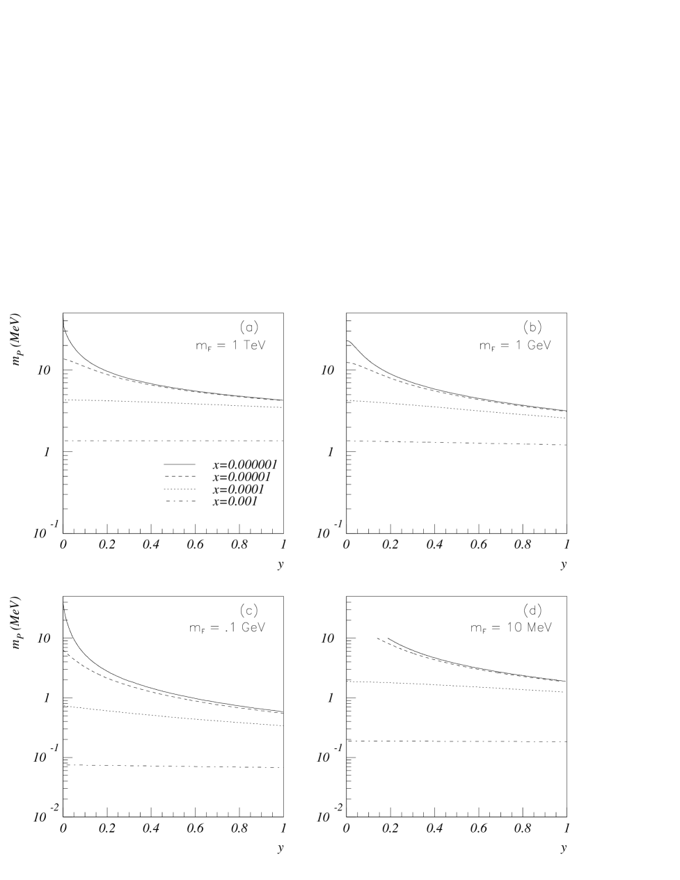
FIG. 1.: Bellow each of the displayed curves, for a fixed value of $x$, we have the allowed region in the plane $m_{F}\times y$, at 90% C. L.  for (a) $m_{F}=$ 1 TeV, (b) $m_{F}=$ 1 GeV, (c) $m_{F}=$ .1 GeV and (d) $m_{F}=$ 10 MeV.

  

FIG. 2.: Maximum allowed value of $m_{P}$ as a function of $x$ for three different values of $m_{F}$ compatible with the neutrinoless double–$\beta$ decay limit.

REFERENCES

• [1] C. Caso et al. (Particle Data Group), Eur. Phys. J.  C3, 1 (1998).
• [2] O. L. G. Peres, V. Pleitez, and R. Zukanovich Funchal, Phys. Rev. D 50, 513 (1994); M. M. Guzzo, O. L. G. Peres, V. Pleitez and R.  Zukanovich Funchal, Phys. Rev. D 53, 2851 (1996); A. Bottino et al., Phys. Rev. D 53, 6361 (1996).
• [3] Since its 1996 edition the Particle Data Group decided not to use the experimental limits on the electron neutrino mass coming from the tritium beta decay experiments due to the difficulty in interpreting the significant negative square mass values in many of these experiments. Their evaluation of the $m_{\nu_{e}}$ limit is dominated by the SN 1987A data. Nevertheless a more stringent limit has been obtained by the Troitsk tritium decay experiment in Phys. Lett. B 350, 263 (1995).
• [4] M. Günther et al., Phys. Rev.  D 55, 54 (1997).
• [5] L. N. Chang, D. Ng, and J. N. Ng, Phys. Rev. D 50, 4589 (1994).
• [6] C. Jarlskog, Nucl. Phys. A518, 129 (1990); Phys. Lett.  B 241, 579 (1990).
• [7] K. S. Babu and E. Ma, Phys. Lett. B 228, 508 (1989).
• [8] D. Choudhury et al., Phys. Rev. D 50, 3468 (1994).
• [9] N. Hata et al., Phys. Rev. D 55, 540 (1997).
• [10] R. R. L. Sharma and N. K. Sharma, Phys. Rev. D 29, 1533 (1984).
• [11] R. Shrock, Phys. Rev. D 24, 1275 (1981); Phys. Lett. B 112, 382 (1982).
• [12] C. O. Escobar, O. L. G. Peres, V. Pleitez and R. Zukanovich Funchal, Phys. Rev. D 47, R1747 (1993).
• [13] P. Kalyniak and J. N. Ng, Phys. Rev. D 24, 1874 (1981).
• [14] G. Degrassi, S. Fanchiotti, and A. Sirlin, Nucl. Phys. B351, 49 (1991).
• [15] M. Finkemeier, Phys. Lett. B 387, 391 (1996).
• [16] W. J. Marciano and A. Sirlin, Phys. Rev. Lett. 71, 3629 (1993).
• [17] K. S. Heard et. al., Phys. Lett. B 55, 327 (1975).
• [18] J. Heintze et. al., Phys. Lett. B 60, 302 (1976).
• [19] R. G. Winter, Lett. Nuovo Cimento 30, 101 (1981).
• [20] The LEP Collaboration ALEPH, DELPHI, L3, OPAL, the LEP Electroweak Working Group and the SLD Heavy Flavour Group: D. Abbaneo et al., CERN-PPE/97-154.
• [21] M. Doi, T. Kotani, and E. Takashugi, Prog. Theor. Phys. Suppl. 83, 1 (1985).
• [22] K. Muto, E. Bender, and H. V. Klapdor, Z. Phys. A334, 187 (1989); A. Staudt, K. Muto, and H. V. Klapdor–Kleingrothaus, Europhys. Lett. 13, 31 (1990).
• [23] A. Halprin, S. T. Petcov, and S. P. Rosen, Phys. Lett. B 125, 335 (1983); A. Halprin, P. Minkowski, H. Primakoff and S. P. Rosen, Phys. Rev. D 13, 2567 (1976).
• [24] W. J. Marciano and A. Sirlin, Phys. Rev. Lett. 56, 22 (1986).