Convergence and Gauge Dependence Properties of the Resummed One-loop Quark-Quark Scattering Amplitude in Perturbative QCD

J.H. Field

Département de Physique Nucléaire et Corpusculaire Université de Genève. 24, quai Ernest-Ansermet CH-1211 Genève 4.

The one-loop QCD effective charge $\alpha_{s}^{eff}$ for quark-quark scattering is derived by diagrammatic resummation of the one-loop amplitude using an arbitary covariant gauge. Except for the particular choice of gauge parameter $\xi=-3$, $\alpha_{s}^{eff}$ is found to increase with increasing physical scale, $Q$, as $\ln Q$ or $\ln^{2}Q$. For $\xi=-3$, $\alpha_{s}^{eff}$ decreases with increasing $Q$ and satisfies a renormalisation group equation. Also, except for the case $\xi=19/9$, convergence radii of geometric series are found to impose upper limits on $Q$.

PACS 12.38-t, 12.38.Bx, 12.38.Cy
Keywords ; Quantum Chromodynamics Renormalisation Group Invariance, Asymptotic Freedom.

1 Introduction

Quark-quark scattering in next-to-leading order QCD has been calculated by several different groups [1-4]. Coqueraux and De Rafael [1], calculated the one-loop corrections to the invariant amplitude in the Feynman gauge using an on-shell renormalisation scheme [5]. In Refs. [2-4] complete expressions for the squared invariant amplitude were given in the dimensional regularisation scheme [6]. The calculations presented in the present paper generalise those of Refs. [1-4] in two ways:

• An arbitary covariant gauge is considered.

• The one-loop Ultra-Violet (UV) divergent loop and vertex diagrams are resummed to all orders in $\alpha_{s}$.

(ii) yields a scale-dependent ‘effective charge’ as a factor in the invariant amplitude. The resummation is done, not by solving a renormalisation group equation (RGE), but by an exact sum of the relevant diagrams to give the QCD analogue of the Dyson sum of QED.

The results are very surprising. The effective charge is gauge dependent at $O(\alpha_{s}^{3})$ and beyond, and except for one specific choice of gauge, does not display ‘asymptotic freedom’ but instead increases as $\ln Q$ or $\ln^{2}Q$ at large scales $Q$. Only for the same special choice of gauge, where contributions from vertex diagrams vanish, does the effective charge satisfy a RGE of the type that is valid in QED [7-11]. For this special choice of gauge (called ‘loop gauge’) the effective charge decreases with increasing scale, but only to a fixed limit $Q_{L}$, determined by the convergence radius of the geometric sum of gluon and fermion loops in the dressed gluon propagator. The measured value of $\alpha_{s}$ suggests that $Q_{L}\simeq$ 300 GeV, already of phenomenological importance at the Fermilab $\rm{p}\overline{\rm{p}}$ collider.

The plan of the paper is as follows. In the next Section the UV divergent (before renormalisation) one-loop corrections to the quark-quark scattering amplitude in Feynman gauge are derived from similar corrections to the quark-quark-gluon vertex given in Ref. [12]. The generalisation to an arbitary covariant gauge is made using results reported in Ref. [13]. In Section 3, the one-loop corrections are diagrammatically resummed to yield the QCD analogue of the Dyson sum of QED. In Section 4 the self-similarity and renormalisation group properties of the effective charge derived in Section 3 are discussed. In the final Section the classical proofs of the asymptotic freedom property of QCD in the literature are critically examined in the light of the results obtained in the previous Sections. Also briefly discussed are : (i) ‘renormalons’ (ii) the generalisation to higher loop order vacuum polarisation and vertex corrections and (iii) pinch technique and related calculations of proper self energy and vertex functions, both in QCD and in the Standard Electroweak Model.

The present paper is the fifth in a series on fundamental physics aspects of perturbative QED and QCD: Ref. [15] discusses on-shell renormalisation and optimised perturbation theory in QED and QCD; Ref. [16] considers the role of non-vanishing fermion or gluon masses as physical regulators for diagrams with combined infra-red (IR) and ultra-violet (UV) divergences; the relation of such IR/UV divergent diagrams to the Lee-Naunberg [17] and Kinoshita [18] Theorems of QED and QCD is examined in Ref. [19]; convergence conditions for resummed physical amplitudes, as discussed in the present paper for quark-quark scattering in QCD, are analysed for the analogous QED case of scattering of unequal mass charged fermions in Ref. [20].

2 The quark-quark scattering amplitude to $O(\alpha_{s}^{2})$ in an arbitary covariant gauge

The process considered is the scattering of two equal mass quarks through an angle of 90^∘ in their CM system. The lowest order diagram is shown in Fig. 1a. The four-vectors of the incoming (outgoing) quarks are $p_{1},p_{2}$ ($p_{3},p_{4}$). In this configuration the exchanged gluon has a virtuality $t=-s/2$ where:

$$t \equiv (p_{1}-p_{3})^{2}=u\equiv(p_{1}-p_{4})^{2},$$ (2.1)

$$s \equiv (p_{1}+p_{2})^{2}=(p_{3}+p_{4})^{2}.$$ (2.2)

Denoting the invariant amplitude corresponding to the diagram in Fig. 1a by ${\cal M}^{(0)}$ (quark spin and colour indices are suppressed), then the $O(\alpha_{s}^{2})$ amplitude may be written as:

$${\cal M}^{(1)}={\cal M}^{(0)}\sum_{i}{\cal A}_{i},$$ (2.3)

where the one-loop virtual corrections ${\cal A}_{i}$ are given by the diagrams shown in Figs. 1b – 1i. Three topologically distinct types of diagrams occur:

• vertex corrections as in Figs. 1b, 1c and the two similar diagrams given by the exchange $13\leftrightarrow 24$;

• loop corrections (Figs. 1d–1g);

• box diagrams (Figs. 1h, 1i).

The leading logarithmic corrections, ${\cal A}_{i}$, corresponding to the contributions of diagrams that are UV divergent before renormalisation, have been derived in a straightforward fashion from the corrections to the quark-quark-gluon vertex presented in Ref. [12]. The results, in Feynman gauge, derived using dimensional regularisation [6] are presented in Table 1. Here $Q=\sqrt{-t}=\sqrt{s/2}$ is the physical scale, and $\mu$ is the renormalistion subtraction scale. $C_{A}$ is the usual QCD colour factor ($C_{A}$ = number of colours = 3) while $n_{f}$ is the number of light quark flavours contributing to the vacuum polarisation loops in Fig. 1d. $\alpha_{s}^{\mu}$ is the square of the renormalised on-shell strong coupling constant at the scale $\mu$. The corrections ${\cal A}_{1}-$${\cal A}_{4}$ may be combined to yield a term proportional to the first coefficient in the perturbation series in $\alpha_{s}$ of the beta function of QCD. Denoting the quark loop + gluon loop + ghost loop correction, ${\cal A}_{3}+{\cal A}_{4}$, by ${\cal L}^{\mu}$, and the vertex correction, ${\cal A}_{1}+{\cal A}_{2}$, by ${\cal V}^{\mu}$, and generalising to an arbitary covariant gauge specified by the parameter $\xi$, in which the gluon propagator is written as :

$$P^{\mu\nu}(q^{2})=-\frac{i}{q^{2}}\left[g^{\mu\nu}-(1-\xi)\frac{q^{\mu}q^{\nu}}{q^{2}}\right]$$ (2.4)

yields the explicit gauge dependence of ${\cal V}^{\mu}$ and ${\cal L}^{\mu}$ [13]

$${\cal V}^{\mu}(\xi) = -\frac{\alpha_{s}^{\mu}}{\pi}\frac{3}{4}(3+\xi)\ln(\frac{Q}{\mu}),$$ (2.5)

$${\cal L}^{\mu}(\xi) = \frac{\alpha_{s}^{\mu}}{\pi}\left[-\frac{3}{4}(\frac{13}{3}-\xi)+\frac{n_{f}}{3}\right]\ln(\frac{Q}{\mu}).$$ (2.6)

Adding Eqs. (2.5) and (2.6):

$${\cal V}^{\mu}(\xi)+{\cal L}^{\mu}(\xi)=-\frac{\alpha_{s}^{\mu}}{\pi}(\frac{11}{2}-\frac{n_{f}}{3})\ln(\frac{Q}{\mu})=-\frac{\alpha_{s}^{\mu}}{\pi}\beta_{0}\ln(\frac{Q}{\mu}),$$ (2.7)

where $\beta_{0}$ is the first coefficient of the QCD $\beta$ function [ $a_{s}\equiv\alpha_{s}/\pi$] :

$$\mu\frac{\partial a_{s}}{\partial\mu}=\beta(a_{s})=-\beta_{0}a_{s}^{2}+...$$ (2.8)

To $O(\alpha_{s}^{2})$, $\alpha_{s}^{Q}$ may be identified with the solution, $\alpha_{s}^{RGE}(Q)$, of the RGE (2.8):

$${\cal M}^{LO} = {\cal M}^{(0)}+{\cal M}^{(1)}={\cal M}^{(0)}(1+{\cal V}^{\mu}(\xi)+{\cal L}^{\mu}(\xi))$$ (2.9)

$$= \frac{{\cal M}^{(0)}}{\alpha_{s}^{\mu}}\left[\alpha_{s}^{\mu}[1-\frac{\alpha_{s}^{\mu}}{\pi}\beta_{0}\ln(\frac{Q}{\mu})]\right]$$

$$= \frac{{\cal M}^{(0)}\alpha_{s}^{RGE}(Q)}{\alpha_{s}^{\mu}}+O\left((\alpha_{s}^{\mu})^{2}\right),$$

where

$$\alpha_{s}^{RGE}(Q)=\alpha_{s}^{Q}=\frac{\alpha_{s}^{\mu}}{1+\frac{\alpha_{s}^{\mu}}{\pi}\beta_{0}\ln(\frac{Q}{\mu})},$$ (2.10)

${\cal M}^{LO}$ denotes the amplitude including Leading Order vertex and vacuum polarisation corrections. In the following section the amplitude ${\cal M}^{(\infty)}$, in which these corrections are summed to all orders in $\alpha_{s}$, is derived.

It can be seen that, at one loop, the gauge invariant result (2.7) is obtained on adding the UV divergent contributions of diagrams (b)–(g) in Fig. 1. The box diagrams (h) and (i) and those obtained by exchanging the internal quark and gluon propagators, form, together with the diagrams where a single gluon is radiated from one of the external quark lines of Fig. 1a, another gauge invariant set. Indeed the contribution to the cross section of this set of diagrams, which involve only abelian quark-gluon couplings, is obtained by multiplying the result for the analogous QED t-channel Bhabha scattering process [22] by the appropriate QCD colour factor: $C_{2}(N_{c})=(N_{c}^{2}-1)/2N_{c}=4/3$. The contribution of the box diagrams alone is UV finite, but IR divergent for the case of massless gluons. This IR divergence is cancelled on adding the contribution of the real gluon radiation diagrams. The contributions of the box diagrams and the real radiation diagrams are however, separately, gauge invariant. Since the box diagrams are UV finite, and so do not require renormalisation, they do not contribute to the QCD effective charge. All the terms that contribute to the latter at one loop are presented in Table 1; they are UV divergent before renormalisation.

3 The resummed quark-quark scattering amplitude

The topographical structures of the diagrams that modify the gluon propagator in the quark-quark scattering amplitude at $O(\alpha_{s}^{2})$, $O(\alpha_{s}^{3})$ and $O(\alpha_{s}^{4})$ are shown in Figs. 2a,b,c respectively. $V$ and $L$ denote vertex and loop (vacuum polarisation) contributions:

$$V = V_{1}+V_{2},$$ (3.1)

$$L = \sum_{i=1}^{n_{f}}F_{i}+G_{1}+G_{2}+G_{3}.$$ (3.2)

$V_{1}$, $V_{2}$ correspond to the diagrams in Fig. 1b, 1c ; $\sum_{i=1}^{n_{f}}F_{i}$ to Fig. 1d and $G_{1}$, $G_{2}$, $G_{3}$ to Figs. 1e,f,g. In the case that only one vertex insertion occurs there is a factor 2 for the two ends of the gluon propagator. Since the propagator has only two ends the vertex corrections are never higher than quadratic in the perturbation series for the amplitude. Although the topographical structure of diagrams containing vertex corrections is different at $O(\alpha_{s}^{3})$ than at $O(\alpha_{s}^{2})$ it remains the same at all higher orders. The all–orders resummed amplitude is:

$${\cal M}^{(\infty)} = {\cal M}^{(0)}\left[1+2V+L\right.$$ (3.3)

$$~{}~{}~{}~{}~{}+V^{2}+2VL+L^{2}$$

$$~{}~{}~{}~{}~{}\left.+V^{2}L+2VL^{2}+L^{3}+...~{}~{}\right]$$

$$= {\cal M}^{(0)}\left[1+L+L^{2}+...+V^{2}\right.(1+L+L^{2}+...$$

$$~{}~{}~{}~{}~{}\left.+2V(1+L+L^{2}+...~{}~{}\right]$$

$$= \frac{{\cal M}^{(0)}(1+V)^{2}}{1-L}.$$

In an arbitary covariant gauge with momentum subtraction at scale $\mu$, and in leading logarithmic approximation, $V={\cal V}^{\mu}(\xi)/2$, $L={\cal L}^{\mu}(\xi)$ so that

$${\cal M}^{(\infty)}=\frac{{\cal M}^{(0)}\alpha_{s}^{eff}(Q)}{\alpha_{s}^{\mu}}=\frac{{\cal M}^{(0)}(1+\frac{1}{2}{\cal V}^{\mu}(\xi))^{2}}{1-{\cal L}^{\mu}(\xi)}$$ (3.4)

leading to the following expression, in leading logarithmic approximation, for the resummed one-loop effective charge:

$$\alpha_{s}^{eff}(Q)=\alpha_{s}^{\mu}\frac{\left[1-\frac{3\alpha_{s}^{\mu}}{8\pi}(3+\xi)\ln(\frac{Q}{\mu})\right]^{2}}{1+\frac{\alpha_{s}^{\mu}}{4\pi}\left[13-3\xi-\frac{4n_{f}}{3}\right]\ln(\frac{Q}{\mu})}.$$ (3.5)

The conventional one-loop QCD running coupling constant Eq. (2.10) is recovered only for the special choice of gauge parameter $\xi=\xi_{L}=-3$ (‘loop gauge’). Only in this case does $\alpha_{s}^{eff}(Q)$ decrease monotonically with increasing $Q$. For any other choice of gauge $\alpha_{s}^{eff}(Q)$ does not show ‘asymptotic freedom’ as $Q\rightarrow\infty$ but instead increases as $\ln Q$ when $\xi\neq\xi_{V}$ and as $\ln^{2}Q$ when $\xi=\xi_{V}$. The choice $\xi=\xi_{V}$ (‘vertex gauge’) where

$$\xi_{V}=(39-4n_{f})/9$$

corresponds to a vanishing coefficient of $\ln(Q/\mu)$ in the denominator of Eq. (3.5). As discussed in more detail below, only in loop gauge is the equation for the effective charge ‘self similar’ like the effective charge in QED or the solution (2.10) of the RGE Eq. (2.8). Even in loop gauge the effective charge of Eq. (3.5) does not decrease without limit as $Q\rightarrow\infty$. The maximum possible scale $Q_{L}$ (Landau scale) is determined by the convergence properties of the geometric sum that yields the denominator of Eq. (3.5). The geometric series is convergent provided that $|L|<1$ [24]. This implies that:

$$\left|\frac{\alpha_{s}^{\mu}}{4\pi}[13-3\xi-\frac{4n_{f}}{3}]\ln(\frac{Q}{\mu})\right|<1.$$ (3.6)

The corresponding Landau scale is then:

$$Q_{L}=\mu\exp\left[\frac{4\pi}{\alpha_{s}^{\mu}[13-3\xi-\frac{4n_{f}}{3}]}\right]$$ (3.7)

and

$$\alpha_{s}^{eff}(Q_{L})=\frac{\alpha_{s}^{\mu}}{2}\left[1-\frac{3\alpha_{s}^{\mu}}{8\pi}(3+\xi)\ln(\frac{Q_{L}}{\mu})\right]^{2}.$$ (3.8)

For $\xi=-3$:

$$\alpha_{s}^{eff}(Q_{L})=\frac{\alpha_{s}^{\mu}}{2},$$ (3.9)

so the convergence condition (3.6) implies that in this case $\alpha_{s}^{eff}$ cannot evolve down by more than a factor of $\frac{1}{2}$ of its initial value before Eq. (3.5) diverges — there is no ‘asymptotic freedom’. The convergence conditions for a geometric series with a negative common ratio, such as that which generates the QCD running coupling constant, are derived below in an Appendix. Unlike in the case of the Landau pole [25] of QED, with a positive common ratio, $r=|r|$, where the running coupling constant is proportional to $1/(1-|r|)$, it is not obvious, by inspection, that the QCD perturbation series is not equal to $1/(1+|r|)$ when $|r|>1$. However (see the Appendix) this is quite clear from the exact formula, Eq. (A1), giving the sum for any finite number of terms. Physicists have the right to be as free as possible in making conjectures in their attempts to describe nature in the simplest way possible, but not to make ones that are contrary to mathematical laws.

Numerical values of $Q_{L}$ for $\mu=5$ GeV, $\alpha_{s}^{\mu}=0.2$ and $n_{f}=5$ (corresponding, approximately, to the experimental value of $\alpha_{s}^{\mu}$) and four different choices of gauge parameter are presented in Table 2. For loop gauge ($\xi=-3$) $Q_{L}$ is only 300 GeV, with phenomenological consequences perhaps already at the Fermilab $\rm{p}\overline{\rm{p}}$ collider, but certainly at the future LHC pp collider. It may be noted that, in all cases except vertex gauge, $Q_{L}$ lies well below the Grand Unification (GUT) scale of $\simeq 10^{15}$ GeV. Since for any gauge choice except $\xi=-3$, $\alpha_{s}^{eff}$ diverges as $\ln Q$ or $\ln^{2}Q$ at large $Q$, there can be no ‘unification’ [26, 27] of the strong and electromagnetic interactions at large scales $Q$, for any choice of gauge parameter, at least if the running strong coupling constant is identified with an effective charge such as that in Eq. (3.5). In fact all studies, to date, of Grand Unification have implicitly used loop gauge where the maximum scale $Q_{L}$ is only $\simeq$ 300 GeV. In vertex gauge, since all vacuum polarisation contributions vanish, there is no convergence limitation on $Q$ in Eq. (3.5).

The behaviour of $\alpha_{s}^{eff}$ at large values of $Q$ depends on the value of the Landau scale and value, $Q_{0}$, of $Q$ at which the numerator of Eq. (3.5) vanishes:

$$Q_{0}=\mu\exp\left[\frac{8\pi}{3\alpha_{s}^{\mu}(3+\xi)}\right].$$ (3.10)

The value of $\xi$, $\xi_{0}$, at which $Q_{L}$ and $Q_{0}$ are equal is given by (3.7) and (3.10) as:

$$\xi_{0}(n_{f})=\frac{1}{9}\left(17-\frac{8n_{f}}{3}\right)$$ (3.11)

For $n_{f}=5$, $\xi_{0}=0.4074...$. When $\xi<\xi_{0}$, (e.g. Loop and Landau gauges) and $Q_{L}<Q_{0}$, then $\alpha_{s}^{eff}$ diverges before vanishing and so decreases monotonically with increasing $Q$ within its convergence radius. For $\xi>\xi_{0}$ (e.g. Feynman and Vertex gauges) $Q_{L}>Q_{0}$. In this case $\alpha_{s}^{eff}$ first decreases with increasing $Q$, reaching a minimum value at zero, and then increases with increasing $Q$ up to $Q_{L}$. In vertex gauge $Q_{L}$ is infinite. Numerical values of $Q_{0}$ for the same parameter choices as in Table 2 are presented in Table 3. The scale $Q_{0}$ is defined (i.e. $Q_{L}>Q_{0}$.) only for Feynman gauge ($Q_{0}=176$ TeV) and Vertex gauge ($Q_{0}=18.1$ TeV).

The diagrams shown in Fig. 2 each contain only a single ‘dressed’ virtual gluon. It is also possible to consider cases in which the subsitution of the series of diagrams illustrated in Fig. 2, and summed in Eq. (3.3), is made in a diagram containing more than one virtual gluon (for example the box diagrams shown in Fig. 1h and 1i). This will result in a further higher order correction to the quark-quark scattering process. It is clear, however, that the manifest gauge dependence of the resummed one-loop contribution will be unaffected by the presence of other virtual gluons (‘dressed’ or not) in the diagram. Every virtual gluon has only two ends, and so the resummed vertex correction is at most quadratic. Then no cancellation is possible of the gauge dependent pieces of multiple vacuum polarisation insertions. However, as further discussed in Section 5 below, the box diagrams themselves can be resummed. This typically results in a Sudakov-like double logarithm, not a geometric series as found for resummed vacuum polarisation diagrams.

4 Self-Similarity Properties of $\alpha_{s}^{eff}$ and the Renormalisation Group

Introducing the abbreviated notation:

$$v(\xi)\equiv\frac{3}{8}(3+\xi)~{}~{}~{},~{}~{}l(\xi)=\frac{1}{4}\left[13-3\xi-\frac{4n_{f}}{3}\right]$$

$$\alpha_{s}^{eff}(Q)/\pi\equiv a_{Q}~{}~{}~{},~{}~{}\alpha_{s}^{\mu}/\pi\equiv a_{\mu}~{}~{}~{},~{}~{}\lambda\equiv\ln(Q/\mu)$$

Eq. (3.5) may be written as:

$$a_{Q}=\frac{a_{\mu}[1-a_{\mu}v(\xi)\lambda]^{2}}{1+a_{\mu}l(\xi)\lambda}.$$ (4.1)

With $\xi=-3$, $v(-3)=0$, Eq. (4.1) becomes

$$a_{Q}=\frac{a_{\mu}}{1+a_{\mu}l(-3)\lambda}.$$ (4.2)

Eq. (4.2) is the solution of a one-loop RGE similar to that for the QED effective charge [10, 11]:

$$\frac{Q}{a_{Q}}\frac{\partial a_{Q}}{\partial Q}=-l(-3)a_{Q}=-\beta_{0}a_{Q},$$ (4.3)

where

$$\beta_{0}=l(-3)=\frac{11}{2}-\frac{n_{f}}{3}.$$ (4.4)

For a gauge choice such that $v\neq 0$ the partial differential equation satisfied by $a_{Q}$ is:

$$\frac{Q}{a_{Q}}\frac{\partial a_{Q}}{\partial Q}=-a_{Q}\left[\frac{l(\xi)}{(1-a_{\mu}v(\xi)\lambda)^{2}}+2\frac{v(\xi)(1+a_{\mu}l(\xi)\lambda)}{(1-a_{\mu}v(\xi)\lambda)^{3}}\right],$$ (4.5)

so that, in this case, the effective charge $a_{Q}$ does not satisfy the RGE (4.3). Expanding in powers of $a_{\mu}$ on the right hand side of Eq. (4.5) gives:

$$\frac{Q}{a_{Q}}\frac{\partial a_{Q}}{\partial Q} = -a_{Q}\left[l(\xi)+2v(\xi)+O(a_{\mu})\right]$$ (4.6)

$$= -a_{Q}\left[\beta_{0}+O(a_{\mu})\right].$$ (4.7)

Thus, neglecting terms of $O(a_{Q}a_{\mu})\simeq O(a_{\mu}^{2})$ so that only the first term in the QCD perturbation series is retained, $a_{Q}\rightarrow a_{Q}^{(1)}$ and it can be seen that $a_{Q}^{(1)}$, for an arbitary gauge choice, satisfies the same partial differential equation as the one-loop all orders resummed $a_{Q}$ in loop gauge. The relation of this result to previous derivations of the QCD running coupling constant, where it has generally been conjectured that a gauge invariant result is obtained to all orders in perturbation theory, is discussed in the following Section.

The equation (4.2) is self-similar in the sense that , for any values of $\mu$ and $Q$ the equation defined by the exchange $\mu\leftrightarrow Q$ is identical to the original equation. A consequence of this symmetry property is that $a_{Q}$ in Eq. (4.2) is independent of $\mu$ (with the important caveat that, since the denominator is the sum to infinity of a geometric series, $\mu$ must be such that $|a_{\mu}l(-3)\lambda|<1$), and that in the equation with $\mu\leftrightarrow Q$, $a_{\mu}$ is independent of Q. This is the mathematical basis of the Renormalisation Group [7, 8, 9]. Such a universal self-similarity property is not, however, shared by Eq. (4.1) when $v(\xi)\neq 0$.

Eq. (4.1) is self-similar under the exchange $\mu\leftrightarrow Q$ provided that the equation:

$$a_{\mu}=\frac{a_{Q}[1+a_{Q}v(\xi)\lambda]^{2}}{1-a_{Q}l(\xi)\lambda}$$ (4.8)

and Eq. (4.1) are both valid. Simultaneous solution of Eqs. (4.1), (4.8) in the case that $v(\xi)\neq 0$ leads to a quadratic equation for $a_{\mu}$ with the solution:

$$a_{\mu}=\frac{1}{v(\xi)\lambda}+\frac{a_{Q}}{2}\pm\frac{1}{2}\sqrt{(\frac{2}{v(\xi)\lambda}+a_{Q})(\frac{2}{v(\xi)\lambda}-3a_{Q})}.$$ (4.9)

Real solutions of Eq. (4.9) exist provided that either

$$\frac{2}{3v(\xi)\lambda}>a_{Q}>-\frac{2}{v(\xi)\lambda}$$ (4.10)

(both factors under the square root positive) or

$$\frac{3v(\xi)\lambda}{2}>\frac{1}{a_{Q}}>-\frac{v(\xi)\lambda}{2}$$ (4.11)

(both factors under the square root negative).

The solution for $a_{\mu}$, Eq. (4.9), is independent of $l(\xi)$. Thus for fixed values of $a_{Q}$, $Q$, $\mu$, $v(\xi)\neq 0$, satisfying the conditions (4.10) or (4.11) there are, in general, two values of $a_{\mu}$ such that Eq. (4.1) is self-similar. This value of $a_{\mu}$ has however no relation to the effective charge at the scale $\mu$ given by Eq. (4.1) when $Q=\mu$. Choosing $Q=90$ GeV and Landau gauge then (see Fig. 3) $a_{Q}=0.095/\pi=0.0302$. The choice $\mu=5$ GeV gives $2/(v(0)\lambda)=1.933$. The $a_{Q}$ terms under the square root of Eq. (4.9) may then be neglected, leading to the solutions:

$$a^{+}_{\mu}\simeq\frac{2}{v(0)\lambda}+\frac{a_{Q}}{2}=1.9648$$

$$a^{-}_{\mu}\simeq\frac{a_{Q}}{2}=0.0152$$

to be compared with the physical value:

$$a_{\mu}=\alpha^{eff}(5{\rm GeV})/\pi=0.2/\pi=0.064$$

Unlike for the special case $v=0$, the first derivative of $a_{Q}$ in general depends on the scale $\mu$. For $Q=\mu$ the derivative is a negative constant fixed by the first coefficient in the perturbation series for the beta function as in Eq. (4.3). For any other choice of $\mu$ when $v\neq 0$ the derivative varies with $Q$ and $\mu$ according to Eq. (4.5). Thus, if the effective charge is parametrised in terms of $a_{\mu}$, $a_{\mu^{\prime}}$ at the reference scale $Q_{R}$:

$$a_{Q_{R}}=a_{\mu}\frac{[1-a_{\mu}v(\xi)\lambda_{R}]}{[1+a_{\mu}l(\xi)\lambda_{R}]}=a_{\mu^{\prime}}\frac{[1-a_{\mu^{\prime}}v(\xi)\lambda_{R}^{\prime}]}{[1+a_{\mu^{\prime}}l(\xi)\lambda_{R}^{\prime}]},$$ (4.12)

$$\lambda_{R}\equiv\ln(Q_{R}/\mu)~{},~{}~{}\lambda_{R}^{\prime}\equiv\ln(Q_{R}/\mu^{\prime})$$

then for $Q\neq Q_{R}$ and $v(\xi)\neq 0$ the effective charge $a_{Q}$ predicted by the formula containing $\mu$ (the second member of Eq. (4.12)) will be different to that predicted by that containing $\mu^{\prime}$ (the third member of Eq. (4.12)), so that the value of $a_{Q}$ depends upon the choice of renormalisation scale — it is no longer invariant. Renormalisation group invariance with respect to the choice of the scale $\mu$ is therefore not respected unless $v(\xi)=0$, i.e. $\xi=-3$.

5 Discussion

In the original derivations of the ‘asymptotic freedom’ property of QCD  [28, 29] no calculations were performed beyond the lowest non-trivial order, $O(\alpha_{s}^{2})$, and no actual amplitudes for physical processes were considered. It was conjectured (without any check by direct diagrammatic calculation) that the QCD running coupling constant (RCC) could, in general (for any choice of gauge) be identified with the solution of the differential equation (2.8). The one-loop QCD beta function was calculated by considering the Callan-Symanzik [10, 11] equation for an irreducible $n$-point function (typically the gluon-quark-quark vertex or the triple gluon vertex). Calculation of the anomalous dimensions of the quark and gluon fields then yields the (gauge invariant) expression for the first beta function coefficient $\beta_{0}$ in Eq. (2.8) above. An analogous result is obtained above by considering the unresummed one-loop correction to the physical quark-quark scattering amplitude. The true high order behaviour, however, corresponds to the sum of all the possible amplitudes for the process of interest. For this the actual topographical structure of the diagrams contributing to the amplitude must be properly taken into account. Renormalisation scale invariance of the RCC, and the asymptotic freedom property, for an arbitary choice of covariant gauge, are not confirmed by the diagrammatic calculation of higher order corrections in the case of the quark-quark scattering amplitude considered in this paper.

Gauge dependence of the RCC in QCD has been considered previously in the literature, but usually as an effect only at the two-loop level and at higher orders. It was pointed out that, in the case when the bare parameters of the theory are held fixed, the gauge parameter becomes scale dependent, and for certain momentum subtraction renormalisation schemes, the second coefficient of the beta function is both scheme and gauge dependent [30]. For an arbitary covariant gauge specified by the fixed parameter $\xi$, as in the one-loop discussion above, the second beta function coefficient is, however, both gauge and renormalisation scheme invariant. Assuming that the RCC, mass and gauge parameter each satisfy renormalisation group equations similar to (2.8), and solving the coupled system of differential equations, solutions were found for the RCC that strongly depended on the initial conditions imposed on the running gauge parameter [30]. These solutions exhibit either asymptotic freedom-like behaviour or increase with increasing scale until an ultraviolet fixed point is reached [31, 32]. As commonly done in the literature, the RCC was treated as an independent mathematical object, without reference to any actual physical process, and the renormalisation group equations were assumed to hold without specific diagrammatic justification. It is shown above that, if the RCC is identified with the effective charge of the quark-quark scattering amplitude, the one-loop renormalisation group equation holds only for the specific gauge choice $\xi=-3$. The gauge parameter can then neither vary nor satisfy a RGE.

When quark mass effects are taken into account, the one-loop beta function coefficient is also gauge dependent, and has a value which depends on the particular $n$-point Green’s function considered for its derivation. The mass dependent corrections to the triple gluon vertex [33] and the gluon-ghost-ghost vertex [34] are different. A detailed discussion may be found in Ref. [35]. A corollary is that the RCC in physical amplitudes is both gauge and process dependent at physical scales where quark mass effects (other than those contained in the asymptotically dominant logarithmic terms) are important.

The effective charge (3.7) has been calculated here for the simple case of quark-quark scattering with a unique physical scale $Q=\sqrt{-t}$. In this case the direct physical interpretation as the strength of the interaction between two currents varying as a function of their separation ($\simeq 1/Q$) is particularly transparent. However, since every dressed propagator has just two ends, similar expressions for the RCC (in general a function of some running loop 4-momentum $k$) are expected in all physical amplitudes containing virtual gluon lines. Two examples are shown in Fig. 4. Fig. 4a shows the three topographically distinct classes of diagrams that contribute to the anomalous magnetic moment of a heavy quark at $O(\alpha_{s}^{3})$. In Fig. 4b the same classes of diagrams are shown for the four-loop photon proper self energy function due to radiatively corrected quark vacuum polarisation loops. As for the quark-quark scattering case the same topographical structures (giving at most a quadratic dependence on the vertex corrections) is found at all higher orders in the ‘dressed gluon propagator’. The diagrams of Fig. 4b are related via the optical theorem and analytical continuation to the process:

$$e^{+}e^{-}\rightarrow\gamma^{*}\rightarrow q\overline{q}+X$$

where $X$ denotes $g$, $gg$ or $q^{\prime}\overline{q}^{\prime}$.

There has been considerable recent interest in the structure, in high orders of perturbation theory, of diagrams containing chains of vacuum polarisation loops in internal gluon propagators (for example the generalisation to higher orders of the $O(\alpha_{s}^{3})$ diagrams with two vacuum polarisation loops shown in Fig. 4). The anstatz used for these so-called ‘renormalon chains’  [36] is to replace $n_{f}/3$ in a calculation considering only $n_{f}$ different flavours of fermion vacuum polarisation loops with $n_{f}/3-11/2=-\beta_{0}$. This is clearly a good approximation in the limit $n_{f}\rightarrow\infty$. As inspection of Fig. 4 shows, however, this will result, in any gauge in which the vertex correction is non-vanishing, in a miscounting of the contribution of the latter, which are included at order $n$ in terms of the form $\beta_{0}^{n}$, but actually should never appear at higher order than quadratic in the perturbation series. With however the gauge choice $\xi=-3$ (loop gauge) all vertex corrections vanish and the renormalon chains are correctly given by the above replacement. This gauge choice is, in any case, the one universally (although tacitly) made in all phenomenological applications of the QCD running coupling constant, where renormalisation group invariance is assumed. Thus the ‘Naive Non-Abelianization’ (NNA) ansatz [37] or ‘Large $\beta_{0}$ Limit’ that is typically assumed in phenomenological studies of renormalon effects is a correct one only in loop gauge. The remark that the choice of gauge $\xi=-3$ implies the vanishing of all vertex corrections, has previously been made in the context of two-loop corrections to heavy quark production in $e^{+}e^{-}$ annihilation [41].

An instructive example of the inconsistent treatment of Feynman diagrams by the NNA anstatz as well as a illustration of the gauge dependence of fixed order perturbative QCD calculations beyond next-to-leading-order (NLO) is provided by the analysis of the moments of non-singlet anomalous dimensions of deep-inelastic nucleon structure functions in Ref. [38]. In this work the effect of insertion of an arbitary number of quark or gluon vacuum polarisation insertions in the virtual gluon propagator of a forward Compton scattering amplitude (or the equivalent diagrams in the Operator Product Expansion, as in Fig. 1 of Ref. [38]) is considered. An example of an O($\alpha_{s}$) diagram that contributes to this amplitude is shown in Fig. 5a. One and two vacuum polarisation loop insertions as considered in Ref. [38] are shown in the fourth topographical diagrams of Fig. 5b and 5d respectively. The predictions of this procedure for the loop ($\xi=-3$) and Landau ($\xi=0$) gauges were compared to the exact massless next-to-next-to-leading-order (NNLO) calculation in Feynman gauge ($\xi=1$) of Ref. [42]. Table 4, extracted from Table 1 of Ref. [38], shows the results of this comparison for the $n=2$ moment at NLO, as in Fig. 5b, and NNLO, as in Fig. 5c and 5d. In the calculations of Ref. [42] the contributions of all 353 Feynman diagrams contributing to the anomalous dimensions up to NNLO were evaluated, whereas in Ref. [38] only quark and gluon loop vacuum polarisation insertions in Fig. 5a and the other Compton scattering diagrams with one virtual gluon line (see for example Fig. 1 of Ref. [43]) were considered. Even so, agreement is found with the Loop gauge renormalon calculation at the 20$\%$ level at NLO for the $n=2$ moment. Even better agreement is found for higher moments —it is good at 4.7 $\%$ for the $n=6$ moment. However, at NNLO no agreement is found; indeed predictions of the ‘renormalon dominated’ approximation with either choice of gauge have even a different sign to the exact NNLO calculation. The reasonable agreement at NLO between the two calculations when loop gauge is employed in Ref. [38] can be understood by inspection of Fig. 5b. This choice of gauge is equivalent, at NLO, to performing a calculation in an arbitary covariant gauge, in which the non-abelian one-loop corrections to the quark-gluon coupling are included as well as vacuum polarisation insertions. All the NLO vertex and vacuum polarisation corrections are included in the topographical diagrams of Fig. 5b. The sum of these contributions is gauge invariant. The situation is quite different at NNLO. The subset of NNLO diagrams shown in Fig. 5c, obtained from those of Fig. 5b by inserting an additional virtual gluon between the incoming and outgoing quark lines also gives a gauge invariant result and is correctly described in loop gauge. This is not the case for the diagrams of Fig. 5d —the corresponding sum of the diagrams is of the form $V^{2}+2VL+L^{2}$, which is manifestly gauge dependent. Other NNLO contributions with the same colour factors as in Table 4 arise from irreducible two-loop vertex and vacuum polarisation diagrams. The topographical pattern is the same as in Fig. 5b with the one-loop insertions replaced by irreducible two-loop insertions. As discussed in more detail below, if these two-loop insertions satisfy a Ward identity similar to that respected by the one-loop insertions, this contribution will also be gauge invariant. No possibility exists however to remove the gauge dependence of the contribution of the diagrams shown in Fig. 5d. This explains the breakdown of gauge invariance shown by the $C_{F}C_{A}^{2}$ NNLO entries of Table 4.

In an attempt to give a diagrammatic justification of the NNA ansatz, Beneke in Ref. [36] considered NLO loop corrections as in Fig. 2a or Fig. 5b above, for the case of quark pair production by a vector current. Performing the calculation in Landau gauge it was found that the beta function of the corresponding QED calculation was replaced by the one-loop QCD beta function. If this calculation had been performed in an arbitary covariant gauge, the gauge invariance of the QCD beta function would have been demonstrated. This in no way justifies the general use of the NNA ansatz since manifest gauge dependence as in Fig. 2b or Fig. 5d first occurs at NNLO where the gauge dependence of the $V^{2}$ term is not cancelled by NNLO vacuum polarisation contributions.

In connection with the work presented in the present paper it is important to notice that the renormalon singularities arise due to loop integrals over the virtuality of an internal photon or gluon line in a Feynman diagram, as in Figs. 4 and 5. Although the renormalon singularities are related to singular IR or UV behaviour of the running coupling constant —as discussed by Lautrup in Ref. [36], in QED it is the UV Landau singularity— the renormalon singularity occurs for arbitary values of the external physical scale due to the infinite range of the internal loop momentum. In contrast, in the simple case of quark-quark scattering discussed in the present paper, there is no integration over the virtuality of the gluon line in which the vertex and loop corrections are inserted and the scale in the running coupling constant is identical to the physical scale of the problem. The diagramatic analysis shown in Fig. 2 is therefore much simpler and the breakdown of gauge invariance appears as soon as the NNLO contributions of Fig. 2b are evaluated.

The classification of diagrams as in Figs. 2, 4 and 5, according to the categories (in an obvious notation) $L^{n},~{}VL^{n},~{}V^{2}L^{n}$, will remain when $L$, $V$ are calculated with an arbitary number of internal lines. The global structure of Eq. (3.5) will then remain the same for calculations including an arbitary number of loops, though additional non-leading terms in $\ln Q$ will result from integration over internal loops in the basic one-loop vacuum polarisation and vertex diagrams shown in Fig. 1.

As in Ref. [1], only the leading logarithmic terms in the one-loop correction (and hence in the resummed effective charge) have been taken into account in the above discussion. Constant terms in $V$ and $L$ have been neglected. For a general renormalisation scheme however, constant gauge and renormalisation scheme dependent terms also occur, so that Eq. (4.1) is replaced by the expression:

$$a_{Q}=a_{\mu}\frac{\{1-a_{\mu}[v(\xi)\lambda+c_{v}(\xi)]\}^{2}}{1+a_{\mu}[l(\xi)\lambda+c_{l}(\xi)]}.$$ (5.1)

In the $\overline{\rm MS}$ scheme [23]:

$$c_{l}(\xi)=\frac{10n_{f}}{9}-\frac{97}{12}-\frac{3}{8}\xi-\frac{3}{16}\xi^{2}$$

By a suitable scale choice $\mu=\mu^{\prime}$ and with $\xi=-3$ Eq. (5.1) may be written as:

$$a_{Q}=\frac{a_{\mu^{\prime}}}{1+a_{\mu^{\prime}}[l(-3)\ln\frac{Q}{\mu^{\prime}}+c_{l}(-3)]}.$$ (5.2)

So in this (non asymptotic) case even in loop gauge the effective charge does not correspond exactly to the solution (2.10) of the one-loop RGE (2.8). Numerically $l(-3)=3.833$, $c_{l}(-3)=-3.090$ for $n_{f}=5$. Thus, in the $\overline{MS}$ scheme in loop gauge, the resummed one-loop invariant charge is only asymptotically a renormalisation group invariant when constant terms in the one-loop correction are retained.

Following the observation that the UV divergent parts of the vertex corrections in Figs. 1b and 1c may be associated with related diagrams in which the virtual quark propagators are shrunk to a point (or ‘pinched’) it was suggested [45, 46] to redefine a gluon proper self energy function by adding to the contributions of Figs. 1d–1g, that of the pinched vertex diagrams. At one-loop order the resulting gluon proper self energy function is then gauge invariant. It was then (incorrectly) stated that a gauge invariant resummed gluon propagator may be trivially derived from the one-loop result (for example, Eq. (2.19) of Ref. [46]). In fact it is easy to show, quite generally, that if the one-loop corrected quark-quark scattering amplitude is gauge invariant (the correct initial assumption of the pinch technique calculations of Refs. [45, 46]) then resummed amplitudes at all higher orders must be gauge dependent. Introducing the gauge invariant one-loop quantity:

$$B\equiv L+2V.$$ (5.3)

The resummed amplitude at O($\alpha_{s}^{n+2}$) may then be written for $n\geq 1$ (see Fig. 2 and Eq. (3.3)) as:

$${\cal M}^{(n+2)}={\cal M}^{(0)}(L+V)^{2}L^{n-1}.$$ (5.4)

Expressing ${\cal M}^{(n+2)}$ in terms of the gauge invariant quantity $B$ and the gauge dependent quantity $L(\xi)$ gives:

$${\cal M}^{(n+2)}={\cal M}^{(0)}\frac{1}{4}(B+L(\xi))^{2}L(\xi)^{n-1},$$ (5.5)

which is manifestly gauge dependent. The Dyson sum in Eq. (2.19) of Ref. [34] correctly describes the all orders resummed amplitude, not for an arbitary gauge parameter $\xi$, but only for the special choice $\xi=-3$ when $V(\xi)=0$, $B=L(-3)$ and

$${\cal M}^{(n+2)}={\cal M}^{(0)}B^{n+1}~{}~{}~{}~{}~{}(\xi=-3).$$ (5.6)

Clearly, the above argument for manifest gauge dependence, shown to be valid at the resummed one-loop level must also hold at arbitary loop order if the vertex and self-energy insertions satisfy a generalised Ward identity giving, at each order of perturbation theory, a condition such as (5.3). It has been shown [47], by the application of background field techniques, that Ward identities relating vertex and self-energy contributions may indeed be derived that are valid to all orders in perturbation theory. The gauge independence of the Ward identity at each fixed order then necessarily implies gauge dependence when the corresponding vertex and self-energy diagrams are resummed.

The manifest gauge dependence of the quark-quark scattering amplitude found, by direct calculation, in this paper, is, apparently, in contradiction with formal proofs [48, 49] of the gauge invariance of $S$–matrix elements in non-abelian gauge theories. It seems however, that what is actually proved in these papers is the gauge invariance, at all orders in perturbation theory, of generalised Ward identities. The consequences of resumming diagrams of fixed loop order, which as shown above, necessarily generates gauge dependence, were not considered. For example, in the standard reference [49], the Lagrangian from which all the Feynman rules of the theory is derived is introduced, and the change in this Lagrangian due to a change in the gauge parameter written down. It is then stated that the theory is gauge invariant if such a variation of the gauge parameter leaves $S$–matrix elements invariant. There immediately follows the statement: ‘We can formulate this condition’ (i.e that the $S$–matrix elements are invariant) ‘in terms of a Ward identity that we have written in terms of the diagrams in Fig. 2’. The unproved and unjustified assertion is thus made that the gauge invariance of a Ward identity is equivalent to gauge invariance of $S$–matrix elements. This will only be true of unresummed amplitudes at each loop order, not of the resummed amplitudes that, according to quantum mechanical superposition, must exist and are, indeed, essential to generate the RCC. In fact Ref. [49] establishes only the gauge invariance of Ward identities, and nothing else. As shown above, it is just the gauge invariance of the unresummed amplitudes that ensure the manifest gauge dependence of the resummed ones. Indeed an $S$–matrix element (even a formal, generic, one) appears nowhere among the equations of Ref. [49]. In Ref. [48] such a formal $S$–matrix element does appear, but its gauge invariance properties are derived directly from a Ward identity. No actual physical process, and no effect of resummation, is considered.

By consideration of a sub-set of $n$-loop diagrams for the off-shell gluon-gluon scattering amplitude in a non-covariant gauge, it has been claimed [23] to demonstrate that the RCC of QCD is both gauge invariant and process independent, and that it may be identified with the solution (2.10) of the RGE (2.8). The $n$-loop diagrams considered are those that may be constructed as a formal ‘product’ of $n+1$ tree level four-point functions. The diagrams contain both resummed one-loop gluon vacuum polarisation and vertex diagrams and a sub set of irreducible $n$-loop diagrams. This set of diagrams cannot, as claimed, be identified with the one-loop RCC in Eq. (2.10), which results solely from the resummation of one-loop (one particle irreducible) diagrams. At any order in the perturbation series these resummed one-loop diagrams contribute the leading powers of both $\ln Q$ and $n_{f}$. They give, in fact, the ‘renormalon’ contribution [36] (see above) that dominates the high order behaviour of the perturbation series. The irreducible $n$-loop ($n>1$) diagrams of the sub-set considered in Ref [23] will contribute constant terms or non-leading powers of $\ln Q$, and therefore cannot be identified with terms in the diagrammatic expansion of the RCC in (2.10). Similarly, it has been conjectured (without explicit calculation) in Ref. [50] that the ‘missing’ vertex contributions needed to make, say, ${\cal M}^{(2)}$ in Eq. (5.5) above, gauge invariant may be derived from ‘pinch parts’ of two-loop irreducible diagrams. This is not possible since the required ‘missing’ contributions contain the factor $(\alpha_{s}\ln Q)^{2}$, (see Eq. (3.5), whereas, as is well known, in both QED [51] and QCD [52] irreducible two-loop vacuum polarisation and vertex diagrams have, at most, next-to-leading logarithmic behaviour $\approx\alpha_{s}^{2}\ln Q$. This is easily demonstrated by considering the two-loop solution of the renormalisation group equation for the effective charge. In QED, or in QCD in the $\xi=-3$ gauge, Eq. (4.2) generalises to:

$$a_{Q}=\frac{a_{\mu}}{1+a_{\mu}\beta_{0}\lambda+\frac{\beta_{1}a_{\mu}}{\beta_{0}}\ln(1+a_{\mu}\beta_{0}\lambda)}~{},$$ (5.7)

where $\beta_{1}$ is the second $\beta$-function coefficient. Expanding the right side of Eq. (5.7) up to $O(a_{\mu}^{3})$ yields:

$$a_{Q}=a_{\mu}\left[1-a_{\mu}\beta_{0}\lambda+a_{\mu}^{2}\beta_{0}^{2}\lambda^{2}-a_{\mu}^{2}\beta_{1}\lambda-a_{\mu}^{3}\beta_{0}^{3}\lambda^{3}+\frac{3}{2}a_{\mu}^{3}\beta_{0}^{3}\beta_{1}\lambda^{2}+O(a_{\mu}^{4})\right].$$ (5.8)

It can be seen that $\beta_{1}$, given by two particle irreducible vacuum polarisation or vertex diagrams, occurs only in sub-leading logarithmic terms of the form $\beta_{1}a_{\mu}^{n}\lambda^{n-1}$. No possible re-arrangement of these terms can compensate the manifest gauge dependence of the leading-logarithmic terms of the form $(\beta_{0}a_{\mu}\lambda)^{n}$.

The property exhibited above, for QCD, of gauge dependence of amplitudes on resumming one-loop corrections that, at lowest order, are gauge invariant, is expected to be a general property of non-abelian gauge theories. In such theories the gauge boson propagator, in an arbitary covariant gauge is written as [53]:

$$P^{\mu\nu}(q^{2})=-\frac{i}{q^{2}-M^{2}}\left[g^{\mu\nu}-(1-\xi)\frac{q^{\mu}q^{\nu}}{q^{2}-\xi M^{2}}\right],$$ (5.9)

where $M$ is the renormalised gauge boson mass. The topographical structure of diagrams contributing to, say, neutrino-neutrino scattering via $Z$ exchange is the same as that for quark-quark scattering shown in Fig. 1. The one-loop vertex correction containing the non-abelian ${Z}{W}^{+}{W}^{-}$ coupling is gauge dependent [54]. Since the gauge dependence cancels at lowest order (without resummation) then, just as for QCD, it cannot cancel at any higher order in the resummed one-loop amplitude. Indeed a similar conclusion as to the necessity of the $\xi=-3$ gauge in order to obtain an effective charge that satisfies a RGE, reached in this paper for QCD, has previously been obtained, for the case of the Weinberg-Salam model, by Baulieu and Coqueraux [55]. These authors pointed out that, with the special gauge choice (in the notation of the present paper) $\xi=-3$, the renormalisation constant of the ${Z}-\gamma$ mixing term vanishes, so that, in this case, effective charges satisfying separate (decoupled) RGE’s may be associated the one-loop resummed photon and $Z$-boson propagators. It is also interesting to note that $\xi=-3$ is the unique choice of covariant gauge for which the photon mass counterterms in the renormalised Lagrangian vanish. The case of $W$ exchange was not considered, but (as may be seen by inspection of the relevant formulae given, in an arbitary covariant gauge, in Ref. [56]) the choice $\xi=-3$ results in the vanishing of the renormalisation constants associated with the one-loop vertex corrections to both the $Z$ and $W$ exchange fermion-fermion scattering amplitudes. As for the QCD case considered in the present paper, it is then expected that, only for this special choice of gauge, an effective charge satisfying a RGE may be associated with the resummed $W$ propagator.

The pinch technique, and similar methods to formally shift gauge dependent pieces between diagrams, have also been applied to electroweak amplitudes [40,46-49]. Although gauge invariant boson proper self energy functions may be defined at one-loop level, any resummed higher order amplitude is demonstrably gauge dependent, by the same argument as that given above for QCD. So, although for a particular choice of gauge parameter (such that the sum of all vertex corrections vanish) resummed $W$ and $Z$ running propagators may be defined that satisfy a RGE, they cannot, contrary to the claim of Refs. [40,46-49], be so defined in a gauge invariant manner. The diagrammatic inconsistency of these procedures is made manifest by the inclusion in the modified vector boson self energy function of box diagram contributions. If the effective charge is expanded as a perturbation series, the box diagram contributions at each order will give terms of a geometric series. There is no way that such a series can be meaningfully interpreted in terms of a sum of such diagrams required by quantum mechanical superposition. In fact, the contributions to physical amplitudes of box diagrams can be systematically resummed [60, 61, 62], but the result found is typically the exponential of a double logarithm of the relevant physical scale, not the sum of a geometric series. For the case of the fermion-fermion scattering amplitude the contribution of box diagrams is expected to be important only in the $|t|\rightarrow 0$ limit and to vanish [56] in the $|t|\rightarrow\infty$ limit.

A discussion of the gauge dependence, beyond one-loop order, of the resonant $Z$ boson amplitude, may be found in Ref. [63].

The limited convergence domain imposed by requiring finiteness of the geometric series, which occurs in all theories in which the RCC decreases with increasing scales, can be avoided by choosing a very high renormalisation scale. This is equivalent, for such theories, to the choice, in QED, of on-shell renormalisation, yielding a RCC that is convergent for all scales below the Landau scale [20]. Although such a choice guarantees convergence for all physical scales below the the chosen renormalisation point, it appears artificial from a physical viewpoint. If a strong interaction process at, say, the scale of the mass of the charm quark is to be described using a renormalisation point at the GUT scale $Q_{\rm GUT}$, the formula for the RCC at scale $m_{c}$ will depend upon the masses of all strongly interacting elementary particles below $Q_{\rm GUT}$ and above $m_{c}$. There will be a phenomenon of ‘inverse decoupling’ whereby the lower the scale the more high mass particles must be taken into account. Feynman amplitudes using such a renormalisation scale would loose their corresponence (valid in the on-shell scheme) with space-time processes. With on-shell renormalisation, the decoupling of heavy particles at low scales is understood in terms of a natural hierachy of physical scales. It seems reasonable that the physics of the strong interaction at the scale of the charm quark mass, $m_{c}$, should be independent of the value of the top quark mass, $m_{t}$, when $m_{t}\gg m_{c}$. According to the the Uncertainty Principle, the contribution to vacuum polarisation loops of particles with masses much greater than the propagator virtuality are expected to correspond to short lifetime fluctuations giving only a small contribution to the radiative correction. This is no longer the case if the RCC is renormalised at scales $\gg m_{t}$.

An enormously successful phenomenology of the strong interaction has been developed over the past three decades based on perturbative QCD. Many aspects of QCD, such as: the existence of the colour quantum number, of spin one gluons with self-coupling, the predicted values of colour factors, and a coupling constant that decreases with increasing scales in the experimentally accessible region, are confirmed, beyond doubt, experimentally [64]. However, it might be hoped that the physical predictions of a candidate gauge theory would be gauge invariant at all orders in perturbation theory, as is the case in QED. Explicit calculation for the current non-abelian gauge theories (both QCD and electro-weak theory), as reviewed in the present paper, seems to show, however, that this is not the case. The point with error bars at $Q=90$ GeV on the loop gauge curve in Fig. 3 shows the uncertainty on $\alpha_{s}$ ($\pm 0.005$) of an early measurement using hadronic $Z$ decays at LEP [65]. The input value $\alpha_{s}(5~{}$GeV$)=0.2$ has been chosen to be consistent with deep inelastic scattering measurements [66]. If the asymptotic running coupling constant with time-like argument measured at LEP at the scale $Q=M_{Z}$ has a similar value to $\alpha_{s}^{eff}(Q)$ for space-like argument considered in this paper, it is clear from Fig. 3 that the measured value of the gauge parameter must be close to $-3$.

On a more positive note, the phenomenological success, in QCD, of calculations based on the renormalisation group, as well as of ‘renormalon’ based models, both of which are shown here to require the use of the $\xi=-3$ gauge, suggests that further understanding requires a deeper theoretical explanation of nature’s apparent choice of this gauge (see Fig. 3). The question is, why, in non-abelian theories, do UV divergent loop diagrams apparently acquire logarithmic corrections after renormalisation but not similar vertex diagrams? Since the non-abelian triple gluon vertex occurs in both loop (vacuum polarisation) and vertex insertions it seems that consistency with experiment requires the cancellation of vertex contributions when summed over the complete particle content of the theory. That is, in some conjectured modified version of QCD, complete cancellation of triangle vertex insertions similar to the anomaly cancellation provided by the particle content of the fermion families of the Standard Model. However, consistency with the diagrammatic description (i.e. with quantum mechanical superposition) must always limit the scale-range of applicability of the RCC due to the convergence properties of geometric series.

Finally, two important caveats concerning the work presented in this paper should be mentioned. Firstly, only covariant gauges specified by the parameter $\xi$ are considered, whereas certain non-covariant gauges [67] such as axial gauge ($A_{3}=0$) or light-cone gauge ($n_{\mu}A^{\mu}=0$, $n^{2}=0$) are freqently employed in QCD phenomenology. The second concerns the recently developed successful application of Analytical Perturbation Theory (APT) to QCD phenomenology [68]. In order to avoid infra-red divergences when $\Lambda\rightarrow 0$ in the conventional QCD perturbation series for the RCC, APT introduces, by way of the Källen-Lehmann spectral representation of the dressed gluon propagator, the condition of analyticity in the $Q^{2}$ variable. This also imposes a causality requirement. In this case, the correspondence between the so-obtained ‘Euclidean running couplant’, $\alpha_{E}$, and the sum of a QCD perturbation series, in which the terms represent the contribution of specific Feynman diagrams, breaks down. No statements may then be made concerning the gauge dependence and convergence properties of $\alpha_{E}$.

6 Acknowledgements

I wish to thank, especially, W.Beenakker for his careful reading of an early version of this paper and for constructively critical comments. Discussions with M.Consoli are also gratefully acknowledged. I thank M.Veltman for pointing out to me the work contained in Ref. [49], and an anonymous referee for introducing me to the related work of Mikhailov discussed in Section 5.

7 Appendix

The sum of the first $n$ terms of a geometric series with a negative common ratio $r=-|r|$ is given by the relation [24]:

$$S_{n}=1-|r|+|r|^{2}-...+(-|r|)^{n-1}=\frac{1-(-|r|)^{n}}{1+|r|}.$$ (A.1)

It follows that:

$$S_{n}=\frac{1+|r|^{n}}{1+|r|}~{}~{}~{}~{}~{}(n-{\rm odd}),$$ (A.2)

$$S_{n}=\frac{1-|r|^{n}}{1+|r|}~{}~{}~{}~{}~{}(n-{\rm even}).$$ (A.3)

If $|r|<1$ , than $S_{\infty}\equiv({\rm limit~{}as}~{}n\rightarrow\infty$ of $S_{n}$) = $1/(1+|r|)$. If $|r|=1$ then $S_{n}=1$ for $n$ odd and $S_{n}=0$ for $n$ even. If $|r|>1$, $S_{\infty}=+\infty$ for $n$ odd and $S_{\infty}=-\infty$ for $n$ even.

Table 4 presents values of $S_{n}$ versus $n$, demonstrating the convergence of the series for $|r|=1/2$ and its divergence for $|r|=2$. The Dyson sum of vacuum polarisation insertions in the gluon propagator in QCD gives a geometric series similar to (A.1) above. The impossiblity of ‘asymptotic freedom’, which conjectures that $S_{n}\rightarrow 0$ as $n\rightarrow\infty$ is evident from inspection of (A.2) and (A.3) above and Table 4.

Tables

i	Diagram in Fig. 1	Type	$(\alpha_{s}^{\mu}/\pi)^{-1}\times$ Correction factor, $A_{i}$, to ${\cal M}^{(0)}$
1	b) + 13 $\leftrightarrow$ 24	abelian vertex	$\frac{C_{A}}{2}\ln\frac{Q}{\mu}$
2	c) + 13 $\leftrightarrow$ 24	non-abelian vertex	$-\frac{3C_{A}}{2}\ln\frac{Q}{\mu}$
3	d)	quark loops	$\frac{n_{f}}{3}\ln\frac{Q}{\mu}$
4	e) + f) + g)	gluon and ghost loops	$-\frac{5C_{A}}{6}\ln\frac{Q}{\mu}$

Table 1: UV divergent (before renormalisation) one-loop virtual corrections, at leading logarithmic accuracy, to the $90^{\circ}$ quark-quark scattering amplitude in Feynman gauge.

Gauge	Feynman ($\xi=1$)	Landau ($\xi=0$)	Loop ($\xi=-3$)	Vertex ($\xi=19/9$)
$Q_{L}$(GeV)	7.68$\times 10^{8}$	1.02$\times 10^{5}$	301	$\infty$

Table 2: Values of the Landau scale $Q_{L}$ (convergence limit) of the QCD effective charge for $\mu=5$ GeV, $\alpha_{s}^{\mu}=0.2$, $n_{f}=5$

Gauge	Feynman ($\xi=1$)	Landau ($\xi=0$)	Loop ($\xi=-3$)	Vertex ($\xi=19/9$)
$Q_{0}$(TeV)	176	Undefined	Undefined	18.1

Table 3: Values of the $Q_{0}$ (the scale at which $\alpha_{s}^{eff}(Q)$ vanishes ). Parameters as in Table 2.

	$\gamma_{(1)}(2)~{}(NLO)$		$\gamma_{(2)}(2)~{}(NNLO)$
Gauge	$C_{F}C_{A}$	$C_{F}N_{f}$	$C_{F}C_{A}^{2}$	$C_{F}C_{A}N_{f}$	$C_{F}N_{f}^{2}$
$\xi=1$	13.9	-$\frac{64}{27}$	117.70	-38.50	-$\frac{224}{243}$
Ref. [42]
$\xi=-3$	11.3	–	-76.0	23.0	–
Ref. [38]
$\xi=0$	7.6	–	-13.2	12.4	–
Ref. [38]

Table 4: Contributions to the $n=2$ moment of the non-singlet anomalous dimension in deep inelastic scattering on a nucleon due to different classes of Feynman diagrams and for different choices of covariant gauge, $\xi$. See text for discussion.

$n$	2	3	4	5	6	7	9	$1/(1+|r|)$
$|r|=1/2$	0.5	0.75	0.625	0.688	0.656	0.673	0.664	0.667
$|r|=2$	-1	3	-5	11	-21	43	-85	0.333

Table 5: Values of the sum, $S_{n}$, of first $n$ terms of the geometric series in (A1) for $|r|=1/2$ (convergent series) and $|r|=2$ (divergent series).

Figure Captions
Fig. 1    Diagrams contributing to ${\cal M}^{(LO)}$. Solid lines denote quarks, wavy lines gluons and the closed loop in g) ghosts.

Fig. 2    The topographical structure of diagrams contributing to the resummed quark-quark scattering amplitude: a) O($\alpha_{s}^{2}$), b) O($\alpha_{s}^{3}$), c) O($\alpha_{s}^{4}$). In diagrams containing only one vertex insertion the contribution given by the exchange $13\leftrightarrow 24$ (see Fig. 1) is understood to be included.

Fig. 3    The variation of the Effective Charge (3.5) with the scale $Q$ for different choices of the gauge parameter $\xi$. 5 GeV $<Q<$ 300 GeV ($\alpha_{s}^{eff}(5~{}\rm{GeV})=0.2$, $n_{f}=5$). The error bars ($\pm$ 0.005) on the point at $Q=90$ GeV on the loop gauge curve are typical of those on an $\alpha_{s}$ measurement using hadronic Z decays [65].

Fig. 4    The topographical structure of diagrams contributing to: a) the O($\alpha_{s}^{3}$) contribution to the anomalous magnetic moment of a quark, b) the four-loop photon proper self energy function.
Fig. 5    The topographical structure of diagrams contributing to non-singlet anomalous dimensions in deep inelastic scattering: a) leading order, b) next-to-leading order, c) and d) next-to-next-to-leading order. See text for discussion.

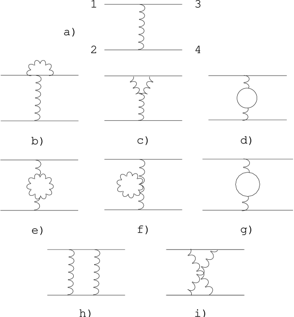
Figure 1: Diagrams contributing to ${\cal M}^{(LO)}$. Solid lines denote quarks, wavy lines gluons and the closed loop in g) ghosts.

Figure 2: The topographical structure of diagrams contributing to the resummed quark-quark scattering amplitude: a) O($\alpha_{s}^{2}$), b) O($\alpha_{s}^{3}$), c) O($\alpha_{s}^{4}$). In diagrams containing only one vertex insertion the contribution given by the exchange $13\leftrightarrow 24$ (see Fig. 1) is understood to be included.

Figure 3: The variation of the Effective Charge (3.5) with the scale $Q$ for different choices of the gauge parameter $\xi$. 5 GeV $<Q<$ 300 GeV ($\alpha_{s}^{eff}(5~{}\rm{GeV})=0.2$, $n_{f}=5$). The error bars ($\pm$ 0.005) on the point at $Q=90$ GeV on the loop gauge curve are typical of those on an $\alpha_{s}$ measurement using hadronic Z decays [65].

Figure 4: The topographical structure of diagrams contributing to: a) the O($\alpha_{s}^{3}$) contribution to the anomalous magnetic moment of a quark, b) the four–loop photon proper self energy function.

Figure 5: The topographical structure of diagrams contributing to non-singlet anomalous dimensions in deep inelastic scattering: a) leading order, b) next-to-leading order, c) and d) next-to-next-to-leading order. See text for discussion.

References

- [1] R. Coqueraux and E. De Rafael, Phys. Lett. 69B, 181 (1977).
- [2] R. K. Ellis et al., Nucl. Phys. B173, 397 (1980).
- [3] W. Slominski and W. Furmanski, Krakow pre-print TPJU-11/81 (1981).
- [4] R. K. Ellis and J. C. Sexton, Nucl. Phys. B269, 445 (1986).
- [5] C. P. Korthals Altes and E. De Rafael, Phys. Lett. 62B, 320 (1976), Nucl. Phys. B125, 275 (1977).
- [6] G. t’Hooft and M. Veltman, Nucl. Phys. B44, 189 (1972).
- [7] E. C. G. Stückelberg and A. Peterman, Helv. Phys. Acta 26, 499 (1953).
- [8] M. Gell-Mann and F. Low, Phys. Rev. 95, 1300 (1954).
- [9] N. N. Bogoliubov and D. V. Shirkov, Nuovo Cimento 3, 845 (1956).
- [10] C. Callan, Jr., Phys. Rev. D2, 1541 (1970).
- [11] K. Symanzik, Comm. Math. Phys. 18, 227 (1970), 23, 49 (1971).
- [12] R. D. Field, ‘Applications of Perturbative QCD’, Addison-Wesley, Redwood City, California, 1989, Chapter 6.
- [13] M. Pennington, Rep. Prog. Phys. 46, 393 (1983).
- [14] C. Itzykson and J-B. Zuber, ‘Quantum Field Theory’ (Mc Graw Hill, New York, 1985).
- [15] J. H. Field, Ann. Phys. (NY) 226, 209 (1993).
- [16] J. H. Field, Int. J. Mod. Phys. A9, 3283 (1994).
- [17] T. D. Lee and M. Nauenberg, Phys. Rev. 133, 1549 (1964).
- [18] T. Kinoshita, J. Math. Phys. 3, 650 (1962).
- [19] J. H. Field, Mod. Phys. Lett. A 11, 2921 (1996).
- [20] J. H. Field, Int. J. Mod. Phys. A15, 3245 (2000).
- [21] J. H. Field, http://xxx.lanl.gov/abs/hep-ph/9811399v1, 9811399v2.
- [22] M. Böhm, A. Denner and W. Hollik, Nucl. Phys. B304, 687 (1988).
- [23] N. J. Watson, Nucl. Phys. B494, 388 (1997).
- [24] G. H. Hardy, ‘Pure Mathematics’ Cambridge University Press 1955, P149.
- [25] A. A. Abrikosov, I. M. Khalatinkov and L. D. Landau, Dokl. Akad. Nauk. SSSR 95, 177 (1954). English translation, paper 80 in ‘Collected Papers’ of L. D. Landau, ed. D. ter Haar, Pergamon Press 1965, Oxford, England.
- [26] H. Georgi and S. L. Glashow, Phys. Rev. Lett. 32, 438 (1974).
- [27] H. Georgi, H. R. Quinn and S. Weinberg, Phys. Rev. Lett. 33, 451 (1974).
- [28] D. Gross and F. Wilczek, Phys. Rev. Lett. 30, 1343 (1973).
- [29] H. D. Politzer, Phys. Rev. Lett. 30, 1346 (1973).
- [30] D. Espriu and R. Tarrach, Phys. Rev. D25, 1073 (1982).
- [31] P. A. Ra̧cza and R. Ra̧cza, Phys. Rev. D39, 643 (1989).
- [32] O. V. Tarasov and D. V. Shirkov, Sov. J. Nucl. Phys. 51, 877 (1990).
- [33] O. Nachtman and W. Wetzel, Nucl. Phys. B146, 273 (1979).
- [34] H. Georgi and H. D. Politzer, Phys. Rev. D14, 1829 (1976). H. D. Politzer, Nucl. Phys. B146, 283 (1976).
- [35] R. Coqueraux, Phys. Rev. D23, 1365 (1981).
- [36] B. Lautrup, Phys. Lett. Phys. Lett. 69B, 107 (1977). G. t’Hooft in The Whys of Subnuclear Physics, Proceedings of the 15th International School of Subnuclear Physics, Erice, Sicily, 1977, edited by A. Zichichi (Plenum New York, 1979). For references to more recent work see, for example, M. Beneke, Phys. Rep. 317, 1 (1999).
- [37] D. J. Broadhurst and A. G. Grazin, Phys. Rev. D52, 4082 (1995).
- [38] S. V. Mikhailov, Phys. Lett. 431B, 387 (1998).
- [39] M. Beneke and V. M. Braun, ‘Renormalons and Power Corrections’ in ‘Physics Handbook of QCD’, Ed. M. Shifman (World Scientific, Singapore, 2001).
- [40] V. M. Braun, E. Gardi and S. Gottwald, Nucl. Phys. B685 171 (2004).
- [41] K. G. Chetyrkin et al., Phys. Lett. 384B, 233 (1996).
- [42] S. A. Larin, T. van Ritbergen and J. A. M. Vermaseren, Nucl. Phys. B427 41 (1994).
- [43] L. Mankiewicz, M. Maul and E. Stein, Phys. Lett. 404B, 387 (1997).
- [44] S. Forte, ‘Progress in Perturbative QCD’ in Proceedings of the 5th International Workshop on Deep-Inelastic Scattering and QCD - DISC ’97 14 - 18 Apr 1997 - Chicago, IL, USA, (New York, NY : AIP, 1997); hep-ph/9706390.
- [45] J. M. Cornwall, Phys. Rev. D26, 1453 (1982).
- [46] J. M. Cornwall and J. Papavassiliou, Phys. Rev. D40, 3474 (1989).
- [47] A. Denner, G. Weiglein and S. Dittmaier, Phys. Lett. 333B, 420 (1996).
-
[48]
B. W. Lee and J. Zinn-Justin, Phys. Rev. D7, 1049 (1973);
E. Abers and B. W. Lee, Phys. Rep. 9C, 127 (1973). - [49] G. t’Hooft and M. Veltman, Nucl. Phys. B50, 318 (1972).
- [50] J. Papavassiliou and A. Pilaftsis, Phys. Rev. D53, 2128 (1996).
- [51] R. Jost and J. M. Luttinger, Helv. Phys. Acta. 23, 201 (1950).
- [52] D. R. T. Jones, Nucl. Phys. B75, 531 (1974).
- [53] G. t’Hooft, Nucl. Phys. B35, 167 (1971).
- [54] G. Degrassi and A. Sirlin, Nucl. Phys. B383, 73 (1992).
- [55] L. Baulieu and R. Coqueraux, Ann. Phys. 140, 163 (1982).
- [56] M. Kuroda, G. Moultaka and D. Schildknekt, Nucl. Phys. B350, 251 (1991).
- [57] D. C. Kennedy et al., Nucl. Phys. 321, 83 (1989); D. C. Kennedy and B. W. Lynn, Nucl. Phys. 322, 1 (1989).
- [58] G. Degrassi and A. Sirlin, Phys. Rev. D46, 3104 (1992).
- [59] J. Papavassiliou, E. de Rafael and N. J. Watson, Nucl. Phys. B503, 79 (1997).
- [60] G. P. Lepage and S. J. Brodsky, Phys. Lett. 87B, 359 (1979).
- [61] M. K. Chase, Nucl. Phys. B189, 461 (1981).
- [62] D. M. Photiadis, Phys. Lett. 164B, 160 (1985).
- [63] M. Passera and A. Sirlin, Phys. Rev. Lett. 77, 4146 (1996).
- [64] See for example the proceedings of the workshop ‘QCD 20 years Later’ Aachen 1992, Ed. P. M. Zerwas, H. A. Kastrup, World Scientific Singapore 1993.
- [65] The LEP Electroweak Working Group, ‘A Combination of Preliminary LEP Electroweak Measurements and Constraints on the Standard Model’, CERN-PPE/95-172.
- [66] M. Virchaux and A. Milsztajn, Phys. Lett. 274B, 221 (1992).
- [67] J.D.Jackson and L.B.Okun, Rev. Mod, Phys. 73, 663 (2001).
- [68] D.V.Shirkov and I.L.Solovtsov, Theor. Math. Phys. 150, 132 (2007), and references therein.