Mass and Coupling Constant Limits from Convergence Conditions on the Effective Charge in QED

J.H.Field

Département de Physique Nucléaire et Corpusculaire Université de Genève . 24, quai Ernest-Ansermet CH-1211 Genève 4.

The massless fermion limit of QED is discussed. For on-shell renormalisation the high energy behaviour fixes no lower limit on the mass of the lightest fermion if the fine structure constant $\alpha$ is allowed to vary. The choice of an arbitary (space-like) subtraction point does, however, fix a lower limit on the mass of the lightest fermion, for any subtraction scale $\mu$, if the effective charge $\alpha^{eff}(\mu)$ respects both quantum mechanical superposition and renormalisation scale invariance. Limits on the values of $\alpha$ or the electron mass are obtained within the Standard Electroweak Model by requiring convergence of $\alpha^{eff}(M_{Z})$.

PACS 12.20-m, 12.20.Ds
Keywords ; Quantum Electrodynamics, Fermion Mass Singularities, Renormalisation Group Invariance, Standard Electroweak Model.

1 Introduction

The massless fermion limit of QED has been discussed in the classic papers of Kinoshita [1] and Lee and Nauenberg [2]. The results contained in these papers are traditionally referred to in the literature as the ‘KLN’ theorem.

The essential conclusion of Kinoshita was the remark that, although unrenormalised Ultra-Violet (UV) divergent amplitudes containing fermion loops are finite in the massless fermion limit, this is no longer the case after charge renormalisation. The renormalised amplitudes contain terms proportional to $\alpha^{2}\ln(Q/m_{f})$ where $\alpha$ is the fine structure constant, $Q$ the physical scale and $m_{f}$ the renormalised fermion mass. For fixed $\alpha$, $Q$ the amplitudes are then logarithmically divergent as $m_{f}\rightarrow 0$. If, however, $\alpha$ and $m_{f}$ are treated as free parameters, then, as discussed below, with a suitable choice for $\alpha$ the divergent part of the amplitude may have any finite value, for any non-zero value of $m_{f}$, however small. Indeed, experimental measurements at scales $\gg m_{f}$ cannot then separately determine $\alpha$ and $m_{f}$. Since, in this case, $m_{f}$ can, in practice, be as small as desired, such a theory is called here ‘quasi-massless’.

Lee and Nauenberg [2] discussed the collinear mass singularities related to the radiation of real photons from external photon lines. They showed, by considering suitable sums of ‘degenerate’ processes (where a fermion line is indistinguishable from a fermion and a collinear photon), that the mass singularities cancel. In the corresponding Feynman diagram calculations, mass singular logarithms appear at intermediate stages of the calculation but cancel, order-by-order in $\alpha$, when real and virtual contributions are added [3]. In the case that the real and virtual diagrams for final state radiation form a gauge invariant set, the cancellation of logarithms is exact. The cancellation does not, however, occur for initial state radiation, or if cuts are applied to the angles and energies of the final state photons.

The KLN theorem has been discussed in some detail in a recent paper by the present author [4] where it is pointed out that uncancelled mass-singular logarithms occur at $O(\alpha^{2})$ in final state radiative corrections due to diagrams where a virtual photon splits into a fermion pair. The corresponding renormalised amplitudes are related via analytical continuation and unitarity cuts to the UV divergent ones discussed by Kinoshita.

In the present paper radiative corrections due to vacuum polarisation loops (forming a gauge invariant set) in the renormalised amplitude for the scattering of unequal mass fermions by one-photon exchange is considered. A similar process ($e$-$\mu$ scattering) was also considered in Ref.[4], using a number of different renormalisation schemes, and where the mass-singular nature of the amplitude for any non-vanishing value of $\alpha$, in accordance with the conclusions of Ref.[1], was confirmed. Here the ‘quasi-massless’ limit of the theory, where $\alpha$ and $m_{f}$ are treated as free parameters, will be considered, as well as constraints derived by requiring convergence of the Dyson sum of the one-loop effective charge for an arbitary renormalisation scale.

The plan of the paper is as follows. In the following Section the information on the value of $\alpha$ and the fermion masses that may be derived from ideal measurements of the differential cross-section of the lepton-lepton scattering process will be considered. In Section 3 the one-loop Renormalisation Group Equation (RGE) for the effective charge $\alpha^{eff}$ is recalled, as well as the relation of its solution to the diagrammatic description of the lepton-lepton scattering amplitude, taking into account radiative corrections due to vacuum polarisation insertions. Requiring convergence of the Dyson sum will be shown to give an upper limit on the renormalisation scale for which the RGE is valid, and also a lower limit on the mass of the lightest fermion. Theories of the ‘quasi-massless’ type are thus excluded if the solution of the RGE is convergent. In Section 4 the phenomenology of the formalism of Section 3 is developed and combined with the Standard Electroweak Model to provide bounds on the fine structure constant or the mass of the lightest fermion.

2 Constraints on $\alpha$ and the Fermion Masses from Measurements of the Effective Charge

The renormalised invariant amplitude for unequal mass charged lepton-lepton scattering, including, to all orders, the effect of one-loop vacuum polarisation insertions: ${\cal M}^{\infty}(Q)$, is related to the effective charge $\alpha^{eff}(Q)$ by the expression:

$${\cal M}^{\infty}(Q)={\cal M}^{0}(Q)\alpha^{eff}(Q)/\alpha$$ (2.1)

where ${\cal M}^{0}(Q)$ is the Born-level amplitude, $\alpha=\alpha^{eff}(0)=1/137.036...$, and $Q$ is the physical scale of the scattering process. Since, at the Born level, only a single diagram contributes to the scattering process, Q is unambiguously defined by the (space-like) virtuality of the exchanged photon (or photons), which is the Mandelstam variable $t$:

$$Q^{2}=-t=(P_{A}-P_{B})^{2}\simeq\frac{s}{2}(1-\cos\theta^{\star})$$ (2.2)

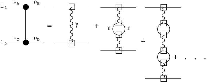
Figure 1: Dyson sum of the 1-loop FVPL generating the effective QED coupling constant in the process $l_{1}l_{2}\rightarrow l_{1}l_{2}$. Open square boxes: renormalised coupling constant with arbitary renormalisation scale. Solid circles: renormalised coupling constant at the physical scale Q. Solid vertical line: dressed photon propagator.

In Eqn.(2.2), $\sqrt{s}$ is the total centre-of-mass energy, $\theta^{\star}$ is the centre-of-mass scattering angle, and the 4-vectors $P_{A}$,$P_{B}$ are defined in Fig.1, which also shows the diagrammatic representation of Eqn.(2.1). The last member of Eqn.(2.2) is valid for $s\gg m_{1}^{2},m_{2}^{2}$ where $m_{1},m_{2}$ are the masses of the leptons $l_{1}$ and $l_{2}$. The effect of including Fermion Vacuum Polarisation Loops (FVPL) to all orders is to replace the ‘bare’ photon propagator of the Born term by the dressed propagator, indicated in Fig.1 by the solid vertical line. The renormalisation scale dependent electric charge of the Born term (represented in Fig.1 by open squares) is replaced by the effective charge at the physical scale $Q$: $e^{eff}(Q)$ (the solid black circles) related to $\alpha^{eff}(Q)$ by:

$$\alpha^{eff}(Q)=e^{eff}(Q)^{2}/4\pi$$ (2.3)

In Eqn.(2.1) the conventional on-shell renormalisation scheme has been used, so that the coupling constant appearing in the Born term is just $\alpha$. The infinite sequence of diagrams shown in Fig.1 gives a geometric series for the effective charge. Using on-shell renormalisation:

$$\alpha^{eff}(Q) = \alpha[1+\Pi_{(Q)}^{(1)}+(\Pi_{(Q)}^{(1)})^{2}+...]$$ (2.4)

$$= \frac{\alpha}{1-\Pi_{(Q)}^{(1)}}$$

Here $\Pi_{(Q)}^{(1)}$ is the one-loop (indicated by the superscript) Photon Proper Self Energy Function (PPSEF) in the on-shell scheme. For $n_{f}$ different species of fermions , of mass $m_{i}$ and charge (in units of that of the positron) $q_{i}$, the PPSEF is given by the expression:

$$\Pi_{(Q)}^{(1)}=\frac{2\alpha}{3\pi}\sum_{i=1}^{n_{f}}q_{i}^{2}{\cal L}(\rho_{i})$$ (2.5)

where $\rho_{i}=Q^{2}/4m_{i}^{2}$ and [5]

$${\cal L}(\rho)\equiv\frac{1}{2}(1-\frac{1}{2\rho})\sqrt{1+\frac{1}{\rho}}\ln\left\{2\sqrt{\rho}[\sqrt{\rho}+\sqrt{1+\rho}]+1\right\}+\frac{1}{2\rho}-\frac{5}{6}$$ (2.6)

For $\rho_{i}\gg 1$ the function ${\cal L}(\rho_{i})$ reduces to the simplified asymptotic form:

$${\cal L}^{\infty}(\rho_{i})=\frac{1}{2}\ln 4\rho_{i}-\frac{5}{6}=\ln\frac{Q}{m_{i}}-\frac{5}{6}$$ (2.7)

On the other hand, for $\rho_{i}\ll 1$, ${\cal L}(\rho_{i})\rightarrow 0$, so that, at low scales, the contributions of heavy fermions to the effective charge decouple.

The contribution of leptons with $|q_{i}|=1$ to the PPSEF is first considered. If there is a hierarchy in the lepton masses such that:

$$m_{1}\ll m_{2}\ll m_{3}~{}....$$

then, away from the ‘threshold’ regions, where $Q\simeq m_{i}$, the effective charge is described by the following simple formula:

$$\frac{1}{\alpha^{eff}(Q)}=-\frac{2n_{f}}{3\pi}\ln\frac{Q}{Q_{L}(n_{f})}$$ (2.8)

where

$$Q_{L}(n_{f})\equiv\overline{m}_{n_{f}}\exp\left[\frac{3\pi}{2n_{f}\alpha}+\frac{5}{6}\right]$$ (2.9)

and

$$\overline{m}_{n_{f}}=\left(m_{1}m_{2}...m_{n_{f}}\right)^{\frac{1}{n_{f}}}$$

Here, $n_{f}$ is the number of active lepton flavours. If $m_{i}\gg Q$, the lepton $i$ is decoupled and therefore ‘inactive’ at the scale $Q$. The evolution of $[\alpha^{eff}(Q)]^{-1}$ for $0\leq Q\leq m_{\tau}$ , according to Eqn.(2.8) is shown in Fig.2. For $Q\simeq m_{e},m_{\mu},m_{\tau}$ the approximation used in Eqn.(2.8) breaks down and the full expression Eqns.(2.4)-(2.6) for the effective charge should be used. The subscript ‘$L$’ on $Q$ in Eqn.(2.9) stands for ‘Landau’, and it can be seen from Eqn.(2.8) that, when $Q=Q_{L}$, the effective charge becomes infinite [6]. As shown in Fig.2, the larger the number of active lepton flavours, the smaller is $Q_{L}$. The Landau scales for 1, 2, 3 active flavours are given by the intersections of the lines L1,L2,L3 with the abscissa $[\alpha^{eff}]^{-1}=0$. The respective scales are: $10^{277}$, $10^{138}$, $10^{93}$ GeV, which may be compared to the Planck scale $Q_{P}$ of 1.22$\times$10¹⁹ GeV. These ‘supra-cosomological’ scales are due to the appearance of $(\alpha)^{-1}$ in the exponential factor in Eqn.(2.9).

The question is now asked:‘What information on the values of the lepton masses and $\alpha$ can be derived from measurements of $\alpha^{eff}(Q)$?’ A semi-realistic gedankenexperiment could simply measure the differential cross-section $d\sigma/dt$ for the lepton-lepton scattering process shown in Fig.1. Applying all QED radiative corrections, except those due to FVPL, to $d\sigma/dt$ yields $d\sigma^{corr}/dt$. The effective charge is then given by the expression:

$$\alpha^{eff}(t)=\left[\frac{1}{2\pi}\frac{s^{2}t^{2}}{s^{2}+u^{2}}\frac{d\sigma^{corr}}{dt}\right]^{\frac{1}{2}}$$ (2.10)

where $u$ is the third Mandelstam variable. Noting that $Q^{2}=-t$, then the masses of the $\mu$ and $\tau$, in the example shown in Fig.2, can be determined by observing the positions of the ‘kinks’ in the logarithmic evolution of $[\alpha^{eff}(Q)]^{-1}$. In fact, it is sufficient to derive the Landau scales $Q_{L}(1)$, $Q_{L}(2)$, $Q_{L}(3)$ from the lines L1,L2,L3 in Fig.2 to determine $m_{\mu}$ and $m_{\tau}$. Eqns.(2.9),(2.10) give:

$$m_{\mu} = \frac{Q_{L}(2)^{2}}{Q_{L}(1)}\exp\left(-\frac{5}{6}\right)$$ (2.11)

$$m_{\tau} = \frac{Q_{L}(3)^{3}}{Q_{L}(2)^{2}}\exp\left(-\frac{5}{6}\right)$$ (2.12)

Unless the experimental resolution is sufficiently good to directly observe the decoupling of the electron the values of $m_{e}$ (the mass of the lightest fermion) and $\alpha$ cannot be separately determined. Their values are, however, constrained by the equation:

$$Q_{L}(1)=m_{e}\exp\left(\frac{3\pi}{2\alpha}+\frac{5}{6}\right)$$ (2.14)

Some value of $\alpha$ can reproduce the measured value of $Q_{L}(1)$ for any value of $m_{e}$, however small. Such a ‘quasi-massless’ theory is indistinguishable from conventional QED for measurements of the effective charge, based on Eqn.(2.10), and sensitive only to scales $Q\gg m_{e}$. Of course, many low energy experimental measurements can easily distinguish between conventional QED and a quasi-massless version with much smaller values of $m_{e}$ and $\alpha$. For example, the energy levels of the hydrogen atom are $\simeq m_{e}\alpha^{2}$. However, the the impact of the actual values of the particle masses on the high energy behaviour of a theory remains of great interest, particularly in view of a similar discussion for QCD, where, because of confinement, no classical limit can be defined.

3 Convergence Properties of the Effective Charge for Arbitary Renormalisation Scales. Renormalisation Group Equations

Making the replacement $Q\rightarrow\mu$ in Eqns.(2.4)-(2.6), and then eliminating the fine structure constant $\alpha$ between the new equations and (2.4)-(2.6), leads to an alternative expression for the effective charge $\alpha^{eff}(Q)$:

$$\alpha^{eff}(Q)=\frac{\alpha^{eff}(\mu)}{1-\frac{2\alpha^{eff}(\mu)}{3\pi}\sum_{i=1}^{n_{f}}q_{i}^{2}[{\cal L}(\rho_{i})-{\cal L}(\tilde{\rho}_{i})]}$$ (3.1)

where

$$\tilde{\rho}_{i}\equiv\frac{\mu^{2}}{4m_{i}^{2}}$$

Since this equation holds for all values of $\mu$, (modulo the convergence constraints to be discussed below), the right side of Eqn.(3.1) is independent of $\mu$. Setting $\mu=0$, for example, Eqns.(2.4)-(2.6) are recovered, as ${\cal L}(\tilde{\rho}_{i})={\cal L}(0)=0$. It is convenient, for the subsequent discussion, to set $Q=0$ and to leave $\mu$ as a free parameter. Since $\alpha^{eff}(0)=\alpha$, Eqn.(3.1) then gives:

$$\alpha=\frac{\alpha^{eff}(\mu)}{1+\frac{2\alpha^{eff}(\mu)}{3\pi}\sum_{i=1}^{n_{f}}q_{i}^{2}{\cal L}(\tilde{\rho}_{i})}$$ (3.2)

What is the physical interpretation of this equation? Referring to Fig. 1 and Eqn.(2.4), the right side of Eqn.(3.2) represents the sum of the series of diagrams with FVPL shown in Fig. 1, but with a different choice of renormalisation subtraction scale; $\mu$ rather than zero as in Eqn.(2.4). Thus the open square boxes in Fig. 1 now represent $e^{eff}(\mu)$ rather than $e^{eff}(0)=e$ as in Eqn.(2.4). Now, Eqn.(3.2) will be consistent with the diagrammatic description provided that the denominator of the right side correctly represents the geometric sum of the Dyson series [8]:

$$\alpha=\frac{\alpha^{eff}(\mu)}{1+\Pi(\mu)}=\alpha^{eff}(\mu)\left[1-\Pi(\mu)+\Pi(\mu)^{2}+...\right]$$ (3.3)

where

$$\Pi(\mu)\equiv\frac{2\alpha^{eff}(\mu)}{3\pi}\sum_{i=1}^{n_{f}}q_{i}^{2}{\cal L}(\tilde{\rho}_{i})$$ (3.4)

The necessary condition for this is that [9]:

$$|\Pi(\mu)|<1$$ (3.5)

The convergence condition (3.5) for the geometric series has the following three consequences:

• For any renormalisation scale $\mu$ Eqn.(3.2) represents a convergent infinite series provided that:

  $$\alpha^{eff}(\mu)<2\alpha.$$

• For any renormalisation scale $\mu$, consistent with the condition given in (i), a definite lower limit on the mass of the lightest fermion exists.

• For any given mass of the lightest fermion, an upper limit exists for $\mu$ consistent with Eqn.(3.5) and the condition given in (i).

For simplicity, the case of a single fermion of mass $m$ and charge $|q|=1$ in the FVPL will be considered. In the subsequent Section the contributions of all known leptons and quarks to the effective charge will be taken into account. With only one active fermion flavour, and $\rho=\mu^{2}/4m^{2}\gg 1$ the convergence condition becomes:

$$\frac{2\alpha_{\mu}}{3\pi}\left[\ln\frac{\mu}{m}-\frac{5}{6}\right]<1$$ (3.6)

where

$$\alpha_{\mu}\equiv\alpha^{eff}(\mu)$$

For fixed $\mu$, the lower limit on $m$ is then

$$m_{MIN}=\mu\exp\left[-\left(\frac{3\pi}{2\alpha_{\mu}}+\frac{5}{6}\right)\right]$$ (3.7)

and for fixed $m$, $\mu$ has the upper limit:

$$\mu_{MAX}=m\exp\left[\left(\frac{3\pi}{2\alpha_{MAX}}+\frac{5}{6}\right)\right]$$ (3.8)

Since, when $m=m_{MIN}$ or $\mu=\mu_{MAX}$, $\alpha_{\mu}=2\alpha$, Eqns.(3.7),(3.8) may also be written:

$$m_{MIN} = \mu\exp\left[-\left(\frac{3\pi}{4\alpha}+\frac{5}{6}\right)\right]$$ (3.9)

$$\mu_{MAX} = m\exp\left[\left(\frac{3\pi}{4\alpha}+\frac{5}{6}\right)\right]$$ (3.10)

The upper limit on the renormalisation scale in Eqn.(3.10), as a function of the values of fermion mass and $\alpha$, is much stronger than that on the physical scale $Q$ found by Landau [6]. For one active lepton flavour, Eqn.(2.9) gives, for the Landau scale:

$$Q_{L}(1)=m\exp\left[\left(\frac{3\pi}{2\alpha}+\frac{5}{6}\right)\right]$$ (3.11)

so that

$$\mu_{MAX}=Q_{L}(1)\exp\left[-\frac{3\pi}{4\alpha}\right]=Q_{L}(1)\times 10^{-140}$$ (3.12)

Since $Q_{L}(1)$ for $m=m_{e}$ is $10^{277}$ GeV, then the corresponding value of $\mu_{MAX}$ is $10^{137}$ GeV, still a supra-cosmological scale much larger than the Planck scale. Setting $\mu=Q_{P}$ in Eqn.(3.9) gives $m_{MIN}=10^{-122}$ GeV, which is the comfortable factor of $2\times 10^{-119}$ below the mass of the electron. Although the convergence condition rigorously excludes theories of the quasi-massless type, its impact on physics in the interesting range of scales $m_{e}<Q<Q_{P}$ would appear to be negligible. As will be explored in more detail below, this is no longer the case if all FVPL contributions are taken into account and $\alpha$ is also treated as a free parameter. For example, setting $m_{MIN}=m_{e}$ and $\mu=Q_{P}$ in Eqn.(3.9) requires that $\alpha<0.046$. So this condition requires that the fine structure constant is ‘small’, no larger than about 6 times its actual value. As shown in Section 4 below, much more restrictive conditions are obtained by including all known vacuum polarisation contributions to the effective charge.

The above considerations may be generalised by choosing an arbitary scale $Q$ in Eqn.(3.1), rather than setting $Q=0$. If the scales $Q$, $\mu$ are large compared to all fermion masses the asymptotic form ${\cal L}^{\infty}$ for ${\cal L}$, Eqn.(2.7), may be used. Then Eqn.(3.1) (with $q_{i}=1$ for all i) may be written as:

$$\alpha_{Q}=\frac{\alpha_{\mu}}{1+\frac{2n_{f}\alpha_{\mu}}{3\pi}\ln\frac{\mu}{Q}}$$ (3.13)

A convergence condition analagous to Eqn.(3.5) then leads to restrictions on the scales $Q$, $\mu$ and the values of $\alpha_{\mu}$ and $\alpha_{Q}$. For $\mu>Q$ these are:

• for fixed Q:

  $$\mu<\mu_{MAX} = Q\exp\left[\frac{3\pi}{4n_{f}\alpha_{Q}}\right]$$ (3.14)

  $$\alpha_{\mu}<\alpha_{MAX} = 2\alpha_{Q}$$ (3.15)

• for fixed $\mu$:

  $$Q>Q_{MIN} = \mu\exp\left[-\frac{3\pi}{2n_{f}\alpha_{\mu}}\right]$$ (3.16)

  $$\alpha_{Q}>\alpha_{MIN} = 0.5\alpha_{\mu}$$ (3.17)

Eq.(3.13) can also be interpreted as a solution of the 1-loop Renormalisation Group Equation (RGE) for the effective charge [10]:

$$Q\frac{\partial a}{\partial Q}=\beta(a)=-ba^{2}$$ (3.18)

where

$$a\equiv\frac{\alpha^{eff}(Q)}{\pi},~{}~{}~{}b=-\frac{2n_{f}}{3}.$$

Now, while it is always true that Eqn.(3.13) is a solution of Eqn.(3.18), whether or not $\mu$ and $Q$ satisfy the restrictions (3.14)-(3.17), the corresponence between the RGE, its solution (3.13), and the geometric sum shown in Fig.1 (which is simply an expression of quantum mechanical superposition) only holds if these restrictions are respected. To show this, consider the contribution $\alpha_{Q}^{n}$ of the first n terms of the Dyson sum:

$$\alpha_{Q}^{n}\equiv\alpha_{\mu}\left[1-R+R^{2}-...+R^{n}\right]=\alpha_{\mu}S_{n}(R)$$ (3.19)

where the common ratio of the geometric series is:

$$R\equiv-b\frac{\alpha_{\mu}}{\pi}\ln\left(\frac{\mu}{Q}\right).$$ (3.20)

The finite sum in (3.19) is:

$$S_{n}(R)\equiv\frac{1}{1+R}-\frac{(-R)^{n+1}}{1+R}$$ (3.21)

while the derivative of $S_{n}$ with respect to R is:

$$\frac{dS_{n}}{dR}=-\frac{1}{(1+R)^{2}}\left\{1-(-R)^{n}[1+n(1+R)]\right\}$$ (3.22)

Eqns.(3.19),(3.20) give:

$$Q\frac{\partial\alpha_{Q}^{n}}{\partial Q}=\frac{\partial\alpha_{Q}^{n}}{\partial\ln Q}=\alpha_{\mu}\frac{dS_{n}}{dR}\frac{\partial R}{\partial\ln Q}=b\frac{\alpha_{\mu}^{2}}{\pi}\frac{dS_{n}}{dR}.$$ (3.23)

The values of $S_{n}(R)$ and $dS_{n}(R)/dR$, in the large n limit, are shown in Table 1 for the five cases:

$$R<-1,~{}~{}~{}R=-1,~{}~{}~{}~{}-1<R<1,~{}~{}~{}R=1,~{}~{}~{}R>1.$$

The asymptotic ($n\rightarrow\infty$) behaviour of $S_{n}(R)$ and $dS_{n}(R)/dR$ may be read off from the entries in Table 1. For $R\leq-1$, $S_{n}\rightarrow\infty$ and $dS_{n}/dR\rightarrow-\infty$. For $-1<R<1$ finite, n independent, values $S_{\infty}$ and $dS_{\infty}/dR$ are found. For $R=1$, $S_{n}(R)$ and $dS_{n}(R)/dR$ exhibit finite oscillations, while for $R>1$ they undergo infinite (sign alternating) oscillations. When $-1<R<1$ (respecting the restrictions (3.14)-(3.17)), $S_{n}(R)$ and $dS_{n}(R)/dR$ are simply related:

$$\frac{dS_{n}}{dR}=-(S_{n})^{2}$$ (3.24)

Thus, using Eqn.(3.24), Eqn.(3.23) can be written, in the $n\rightarrow\infty$ limit, as:

$$Q\frac{\partial\alpha_{Q}^{\infty}}{\partial Q}=-b\frac{\alpha_{\mu}^{2}}{\pi}S_{\infty}^{2}=-\frac{b}{\pi}\left(\alpha_{Q}^{\infty}\right)^{2}$$ (3.25)

which is equivalent to the RGE (3.18). For any other value of $R$, the partial differential equation (3.23) has no finite limit as $n\rightarrow\infty$ and no RGE is obtained. It may be remarked that only for $-1<R<1$ does the right side of Eqn.(3.13) correctly represent the infinite sum $S_{\infty}$. As shown in Table 1, the formula is correct for $-1<R<1$. For $R=-1$, the correct result, $+\infty$, is also found. However, for $R<-1$, Eqn.(3.13) gives a finite negative value instead of the the correct value $+\infty$. For $R=1$ the value of 1/2 is found instead of a value oscillating between 0 and 1, and, finally, for $R>1$, Eqn.(3.13) gives a finite number between 1/2 and 0 instead of the correct (infinitely oscillating) result. Only when $R=-1$ (corresponding, in the analagous case of Eqn.(2.4), to the Landau singularity) is the breakdown of convergence evident from Eqn.(3.13) itself.

The essential conclusion of this Section is that the formula (3.1) for the effective charge corresponds to a finite Dyson sum only for values of the renormalisation subtraction scale $\mu$ less than some upper limit. This limit is fixed either by the mass of the fermion in the FVPL (Eqn.(3.8)) or by the physical scale $Q$ (Eqn.(3.14)). For a fixed renormalisation scale there are complementary lower limits on the fermion mass (Eqn.(3.9)) or $Q$ (Eqn.(3.16)). The upper limit on the renormalisation scale determined by the electron mass and $\alpha$ is, although still of supra-cosmological magnitude, a factor of $10^{140}$ smaller than the Landau scale that fixes the upper limit on $Q$. The RGE for the effective charge is only valid within the convergence domain of the renormalisation scale, so Renormalisation Group Invariance [11] is similarly limited.

In the following Section, constraints on the mass of the lightest fermion and the value of $\alpha$ are derived by applying the convergence condition (3.5) to the effective charge, taking into account all known 1-loop FVPL contributions.

4 Constraints on $\alpha$ and $m_{e}$ from Convergence Conditions on the Effective Charge in the Standard Electroweak Model

The convergence condition (3.5) implies that the relation between the the renormalisation scale $\mu$ and the minimum mass of the lightest fermion (i.e. the electron) $m_{MIN}$, is given by the following expressions:

$$m_{MIN} = \mu\exp\left[-\frac{1}{2}\left(\frac{3\pi}{2\alpha}-F(\mu)\right)\right]$$ (4.1)

$$F(\mu) = 2\ln\frac{\mu^{2}}{m_{\mu}m_{\tau}}+2\ln\frac{\mu}{\overline{m}_{d}}+\frac{16}{3}\ln\frac{\mu}{\overline{m}_{u}}-\frac{100}{9}$$ (4.2)

where

$$\overline{m}_{d}=(m_{s}m_{d}m_{b})^{\frac{1}{3}},~{}~{}~{}\overline{m}_{u}=(m_{u}m_{c})^{\frac{1}{2}}$$

and

$$m_{f}\ll\mu<M_{W},m_{t}$$

so that the top quark contribution and the (gauge dependent) $W$ contributions to the effective charge may be neglected. Eqn.(4.1) is the generalistion, including all known fundamental fermion species, of Eqn.(3.9) where only one fermion species is included in the FVPL. The values of the fermion mass parameters used below in Eqn.(4.2) are presented in Table 2. For each quark flavour, 3 species of fermions are included in Eqn.(3.1) to take into account the colour quantum number of QCD. As is common practice [12], the light quark masses $m_{u}=m_{d},m_{s}$ are chosen so as to correctly reproduce the non-perturbative hadronic vacuum polarisation contribution deduced, via a dispersion relation, from the experimental data on $e^{+}e^{-}\rightarrow$ hadrons. The quark and lepton masses in Table 2, when substituted in Eqn.(2.4) give:

$$\alpha^{eff}(M_{Z})^{-1}=128.9$$

in agreement with recent estimates [13]. The Z mass is taken to be 91.2 GeV [14].

In the Standard Electroweak Model (SM) [15], $\alpha$ and $M_{Z}$ are related by the expression:

$$M_{Z}^{2}=\frac{4\pi\alpha\upsilon^{2}}{\sin^{2}2\theta_{W}}$$ (4.3)

where $\theta_{W}$ is the weak mixing angle and $\upsilon$ is the vacuum expectation value of the Higgs field. The on-shell renormalisation scheme is used, so that:

$$\sin^{2}\theta_{W}=1-\frac{M_{W}^{2}}{M_{Z}^{2}}$$ (4.4)

and virtual electroweak corrections are neglected.

An upper limit, $\alpha_{MAX}$, on the value of the fine structure constant is now obtained by requiring that $\alpha^{eff}(M_{Z})$ is convergent in the sense discussed above . The limit obtained depends on the value of the remaining SM parameters: $\upsilon$ and $\theta_{W}$. Two different hypotheses will be made. Firstly, that $\upsilon$ is fixed at its measured value of $\simeq 252$GeV and only $\theta_{W}$ varies. Since

$$G=\frac{1}{\sqrt{2}\upsilon^{2}}$$ (4.5)

where $G$ is the Fermi constant, the strength of the low-energy weak interaction remains unchanged in this case. Secondly, the parameter $\upsilon^{\prime}$ defined as:

$$\upsilon^{\prime}=\frac{2\sqrt{\pi}\upsilon}{\sin 2\theta_{W}}$$ (4.6)

is allowed to vary freely. Using Eqns.(4.1),(4.3) and (4.6) $\alpha^{eff}(M_{Z})$ is found to be convergent provided that $\alpha<\alpha^{MAX}$ where, with $m_{MIN}=m_{e}$:

$$\frac{\upsilon^{\prime}x}{m_{e}}=\exp\left[\frac{1}{2}\left(\frac{3\pi}{2x^{2}}-F(\upsilon^{\prime}x)\right)\right]$$ (4.7)

and

$$x\equiv(\alpha^{MAX})^{\frac{1}{2}}$$ (4.8)

For fixed $\upsilon^{\prime}$ Eqn.(4.7) is an implict equation for $\alpha^{MAX}$ that is readily solved numerically. The results are shown, as a function of $\sin\theta_{W}$, for $\upsilon=252.2$ GeV, in Fig. 3 and also, as a function of $\upsilon^{\prime}$, in Fig. 4. Also shown, in each case, is the value of $M_{Z}$ given by Eqn.(4.3) when $\alpha=\alpha^{MAX}$. For the experimentally measured values of $\sin\theta_{W}$ and $\upsilon^{\prime}$ (indicated by the vertical arrow) $\alpha^{MAX}$ is $\simeq 0.05$ (i.e. $\simeq 7\alpha$) and $M_{Z}^{MAX}$ is $\simeq 250$ GeV. For smaller values of $\sin\theta_{W}$ (or larger values of $\upsilon^{\prime}$) a marginally stronger restriction on $\alpha$ is obtained. Note that the minimum value of $\upsilon^{\prime}$ for constant $\upsilon$ (and hence the strongest restriction on $M_{Z}$) is obtained when $\sin 2\theta_{W}=1$ or $\theta_{W}=\pi/4$. This limit is indicated by the hatched vertical line in Fig. 3.

Fixing the value of the fine structure constant to its experimental value $\alpha^{exp}$, Eqn.(4.7), with the replacement $x\rightarrow\sqrt{\alpha^{exp}}$, may be solved for the minimum value of the electron mass such that $\alpha^{eff}(M_{Z})$ is covergent. The results, for different values of $M_{Z}$, are presented in Table 3. The corresponding values of $\upsilon^{\prime}=M_{Z}/\sqrt{\alpha^{exp}}$ are also shown. At the actual value of the Z mass, corresponding to $\upsilon^{\prime}=1068$ GeV, the minimum value of the electron mass is 1.9$\times 10^{-128}$ GeV. It is interesting to note that, when all known fermions are included in the FVPL, the minimum electron mass, at a scale of 853 GeV, is 1.1$\times 10^{-120}$ GeV, a factor 100 times greater than the minimum mass at the Planck scale of 1.22$\times 10^{19}$ GeV, given by Eqn.(3.9), where only one fermion species is considered. The convergence conditions become very much more restrictive when additional fermion species are included in the FVPL.

5 Higher Order Corrections

In the on-shell scheme the asymptotic PPSEF for a single fermion species is given, up to two loops, by the expression [16]:

$$\Pi^{(2)}(Q)=\frac{2\alpha}{3\pi}\left[\ln\left(\frac{Q}{m}\right)-\frac{5}{6}\right]+\left(\frac{\alpha}{\pi}\right)^{2}\left[\frac{1}{2}\ln\left(\frac{Q}{m}\right)+\zeta(3)-\frac{5}{24}\right]$$ (5.1)

More generally, the next-to-leading logarithmic contribution to the PPSEF at order $\alpha^{n}$ is [17]:

$$\alpha^{n}\tilde{\Pi}^{(2n)}=\frac{3}{4}\left(\frac{\alpha}{\pi}\right)^{n}\frac{1}{(n-1)}\left[\frac{2}{3}\ln\left(\frac{Q}{m}\right)\right]^{n-1}$$ (5.2)

The terms given by (5.2) for successive values of $n$ are those of a logarithmic series. Thus, the next-to-leading logarithms may be resummed to all orders in $\alpha$ to yield the effective charge, to next-to-leading logarithmic order  [18]:

$$\alpha_{NLL}^{eff}(Q)=\frac{\alpha}{1-\Pi^{(1,\infty)}_{(Q)}+\frac{3\alpha}{4\pi}\ln(1-\Pi^{(1,\infty)}_{(Q)})}$$ (5.3)

where $\Pi^{(1,\infty)}_{(Q)}$ is the asymptotic form of the one loop PPSEF of Eqn.(2.5).

The effect of the next-to-leading logarithmic terms is very small. For example, requiring positivity of the effective charge in Eqn.(5.3) leads to the condition:

$$\Pi^{(1,\infty)}_{(Q)}<0.9917$$

instead of the corresponding one-loop condition $\Pi^{(1,\infty)}_{(Q)}<1$. The Landau scale for one active flavour ($m_{1}=m_{e}$) is reduced from $10^{277}$ GeV to $10^{275}$ GeV. Similar corrections of $\leq 1\%$ are expected in the value of $\Pi(\mu)$ given by the convergence condition (3.5) due to next-to-leading logarithmic terms. This is much less than other sources of error (for, example due to the approximate parameterisation of non-perturbative QCD effects by effective quark masses) in the phenomenological discussion of Section 4 above. In fact, for energy scales of current experimental interest the next-to-leading logarithmic terms in Eqn.(5.3) give a simple multiplicative correction to the one-loop PPSEF. Considering, for example, one fermion flavour ($m_{1}=m_{e}$) and $Q=2$ TeV gives $\Pi^{(1,\infty)}=0.022$. Then, since for small $x$, $\ln(1-x)\simeq-x$, the next-to-leading logarithmic correction modifies the one-loop PPSEF by the constant factor: $1+3\alpha/(4\pi)=1.00742$.

6 Concluding Remarks

This study has shown that, in QED, complementary limits exist bounding from below the mass of the lightest fermion, and from above the the high energy scale at which the theory may be applied, if the freedom of choice of subtraction scale, that leads to Renormalisation Group Invariance, is respected. For smaller masses and higher scales, the geometric series (a consequence of quantum mechanical superposition) that yields the effective charge is not convergent, and the usual relation between the Dyson sum and the solution of the RGE breaks down. The limitations found in this way are much more restrictive than those considered by Landau [6] using the conventional on-shell scheme with a fixed subtraction point.

The work described here may be extended in two different directions:

• Within QED, consider the effect of multiple fermion loop effects in the PPSEF, and contributions due to W loops.

• Apply a similar analysis to the weak and strong interactions.

As discussed in the previous section, even the leading correction of the type (i), due to next-to-leading logarithmic corrections, is small. On the other hand (ii) may be expected to lead to more interesting results. Replacing the invariant amplitude for charged lepton scattering considered here by the respective processes: $\nu_{l}l^{\prime}\rightarrow\nu_{l}l^{\prime}$, $\nu_{l}l^{\prime}\rightarrow\nu_{l^{\prime}}l$ and $qq^{\prime}\rightarrow qq^{\prime}$, the weak neutral current (Z exchange), weak charged current (W exchange) and the strong interaction (gluon exchange) may be investigated. In each of these processes, a single diagram contibutes at the Born level ,and, as in the QED case considered above, there is a unique physical scale in the corresponding ‘running coupling constant’. The analysis of the latter, the analogue, for the weak or strong interactions, of the effective charge of QED, is complicated by problems of gauge dependence. These have been discussed, for neutral currents in the SM, by Baulieu and Coqueraux [19]. Because of $\gamma-Z$ mixing effects, it was concluded that only for a specific choice of covariant gauge $a=\xi^{-1}=-3$ can effective charges respecting a RGE be associated with the photon and Z propagators.

In the case of QCD, although gluon and quark loops are expected to yield a geometric Dyson sum, the gluon loop contribution is gauge dependent, and UV divergent vertex diagrams containing the non-abelian triple gluon coupling must also be taken into account. Qualitatively, the result for the running coupling constant is expected to be determined by a geometric sum of the type:

$$1-R+R^{2}-...=\frac{1}{1+R}$$ (6.1)

(where R is $>0$) in contrast to QED where the corresponding series has the form:

$$1+R+R^{2}+...=\frac{1}{1-R}$$ (6.2)

As is well known, the difference in the sign of $R$ in Eqns.(6.1),(6.2) comes from the dominant contribution, in QCD, of diagrams containing the triple gluon coupling, which have the opposite sign (as in the case of W-pair loops in QED) to the fermion loops [20]. Comparing Eqns.(6.1) and (6.2) it can be seen that there is no Landau singularity in QCD, where the coupling constant becomes infinite, but that a physical limitation will come rather from the convergence of the series in Eqn.(6.1), which is of the same type as that discussed above in connection with the domain of validity of the Renormalisation Group in QED. This problem has been investigated in a companion paper [21]. In view of the relatively large size of the QCD coupling constant it is to be expected, and indeed found, that much more stringent restrictions apply than the Landau condition in QED.

Acknowledgements

W.Beenakker and M.Consoli are thanked for their interest in the work described in this paper and for helpful discussions and correspondence.

	$R<-1$	$R=-1$	$-1<R<1$	$R=1$	$R>1$
$S_{n}$	$\frac{-(-R)^{n+1}}{1+R}$	n+1	$\frac{1}{1+R}$	1 (n even)	$\frac{-(-R)^{n+1}}{1+R}$
				0 (n odd)
$\frac{dS_{n}}{dR}$	$\frac{n(-R)^{n}}{1+R}$	$-\frac{n(n+1)}{2}$	$\frac{-1}{(1+R)^{2}}$	$n/2$ (n even)	$\frac{n(-R)^{n}}{1+R}$
				$-(n+1)/2$ (n odd)

Table 1: Values of the sum $S_{n}$ of a geometric series and of $dS_{n}/dR$, in the large $n$ limit, for different values of the common ratio $R$.

Fermion	e	$\mu$	$\tau$	u	d	s	c	b	t
Mass (MeV)	0.511	105.7	1777	36.9	36.9	500	1570	4906	1.8$\times 10^{5}$

Table 2: Fermion mass parameters used for the vacuum polarisation loops. $\overline{m}_{d}=(m_{s}m_{d}m_{b})^{\frac{1}{3}}$. For $\mu<m_{t}$, $\overline{m}_{u}=(m_{u}m_{c})^{\frac{1}{2}}$. For $\geq m_{t}$, $\overline{m}_{u}=(m_{u}m_{c}m_{t})^{\frac{1}{3}}$

$M_{Z}$ (GeV)	17.1	34.2	91.3	171.0	427.6	853.2
$\upsilon^{\prime}$ (GeV)	200	400	1068	2000	5000	10000
$m_{e}^{MIN}$ (GeV)	5.4$\times 10^{-127}$	5.5$\times 10^{-135}$	1.9$\times 10^{-128}$	2.9$\times 10^{-126}$	6.4$\times 10^{-123}$	1.1$\times 10^{-120}$

Table 3: Minimum values of the electron mass for convergence of $\alpha^{eff}(M_{Z})$, for different values of $M_{Z}$, in the Standard Electroweak Model. $M_{Z}=\sqrt{\alpha}\upsilon^{\prime}$.

Figure 2: $[\alpha^{eff}(Q)]^{-1}$ versus lnQ (MeV), showing the decoupling of the FVPL due to $\tau$, $\mu$, $e$. Quark contributions are neglected. The solid lines indicate regions where the asymptotic formula (2.8) is valid.

Figure 3: Upper limits on the fine structure constant, $\alpha$, and the Z mass, $M_{Z}$ in the Standard Electroweak Model as a function of $\sin\theta_{W}$ (see text). $\upsilon=252.2$ GeV is assumed. The vertical arrow shows the experimental value of $\sin\theta_{W}$. The cross-hatched theoretical bound corresponds to the minimum value of $M_{Z}^{MAX}$ and the maximum value of $\alpha^{MAX}$, obtained when $\sin\theta_{W}=1/\sqrt{2}$.

Figure 4: Upper limits on the fine structure constant $\alpha$ and the Z mass $M_{Z}$ in the Standard Electroweak Model as a function of $\ln\upsilon^{\prime}$ (GeV) (see text). The vertical arrow shows the experimental value of $\ln\upsilon^{\prime}$.

References

- [1] T.Kinoshita, J. Math. Phys. 3, 650 (1962).
- [2] T.D.Lee and M.Nauenberg, Phys. Rev. 133, 1549 (1964).
- [3] For example, this cancellation in the O() correction to is explicitly demonstrated in F.A.Berends, R.Kleiss and S.Jadach, Nucl. Phys. B202, 63 (1982).
- [4] J.H.Field, Mod. Phys. Lett. A. Vol. 11, No 37 2921 (1996).
- [5] J.M.Jauch and F.Röhrlich,‘The Theory of Photons and Electrons’, P. 194, Springer-Verlag, New York/Berlin 1976.
- [6] A.A.Akrikosov, I.M.Khatatinkov and D.Landau, Dokl. Akad. Nauk. SSSR 95, 177 (1954). English translation, paper 80 in ‘Collected Papers’ of L.D.Landau, ed. D. ter Haar, Pergamon Press 1965, Oxford, England.
- [7] J.H.Field, Int Journ. Mod. Phys., A9 3283, (1994).
- [8] F.J.Dyson, Phys. Rev. 75, 486 (1949).
- [9] G.H.Hardy,‘Pure Mathematics’, Cambridge University Press 1955, Cambridge, England, P149.
- [10] C.Callan, Jr. Phys. Rev. D2, 154 (1970). K.Symanzik, Commun. Math. Phys. 18, 227 (1970); 23, 49 (1971).
- [11] E.C.G.Stueckelberg and A.Petermann, Helv. Phys. Acta 26, 499 (1953). M.Gell-Mann and F.Low,Phys. Rev. 95, 1300 (1954). N.N. Bogoliubov and D.V.Shirkov, Dokl. AN SSSR 103, 203 (1955), Nuovo Cimento 3, 845 (1956).
- [12] See, for example, M.Böhm, A.Denner and W.Hollik, Nucl. Phys. 304 687 (1988).
- [13] S.Eidelman and F.Jegerlehner, Z. Phys. C67, 585 (1995). H.Burkhardt and B.Pietrzyk, Phys. Lett. B356, 398 (1995).
- [14] Particle Data Group, C.Caso et al. Eur. Phys. J. C3, 1 (1998).
-
[15]
S.L.Glashow, Nucl. Phys. 22, 579 (1961).
S.Weinberg Phys. Rev. Lett. 19, 1264 (1967).
A.Salam in ‘Elementary Particle Theory’ Ed. N.Svartholm, Almqvist and Wiksell 1968, Stockholm, P367. - [16] R.Jost and J.M.Luttinger, Helv. Phys. Acta 23, 201 (1950).
- [17] E. De Rafael and J.L.Rosner, Ann. of Phys. 82, 369 (1974).
- [18] See the third reference in [11].
- [19] L.Baulieu and R.Coqueraux, Ann. of Phys. 140, 163 (1982).
- [20] D.Gross and F.Wilczek, Phys. Rev. Lett, 30, 1343 (1973). H.Politzer, Phys. Rev. Lett, 30, 1346 (1973).
- [21] J.H.Field,‘Convergence and Gauge Dependence Properties of the One-Loop Resummed Quark-Quark Scattering Amplitude in Perturbative QCD’, University of Geneva pre-print UGVA-DPNC 1997/2-171 (hep-ph/9811399).