Abstract

Data from atmospheric and solar neutrinos indicate that there are at least three neutrino types involved in oscillation phenomena. Even if the corresponding neutrino mass scales are very different, the inevitable reference to mixing between more than two neutrino types has profound consequences on the planning of the accelerator experiments suggested by these results. We discuss the measurement of mixing angles and CP phases in the context of the neutrino beam emanating from a neutrino factory: the straight sections of a muon storage ring. We emphasize the importance of charge identification. The appearance of wrong sign muons in a long baseline experiment may provide a powerful test of neutrino oscillations in the mass-difference range indicated by atmospheric-neutrino observations.

1 Motivation in the current situation

Recently published strong indications of atmospheric neutrino oscillations [1] have rekindled the interest in accelerator experiments that could study the same range of parameter space. The results of SuperKamiokande are interpreted as oscillations of muon neutrinos into neutrinos that are not $\nu_{e}$s. Roughly speaking, the measured mixing angle is close to maximal: $\sin^{2}2\theta>0.8$, and $\Delta m^{2}$ is in the range $5\times 10^{-4}$ to $6\times 10^{-3}$ eV², all at 90% confidence.

The SuperK mass (squared) range is one order of magnitude below the previous Kamiokande observations [2], just what is needed to render the oft-discussed long baseline experiments –such as MINOS [3] or a CERN to Gran Sasso [4] project– hardly capable of covering the whole parameter range of interest.

The solar neutrino deficit is interpreted either as MSW (matter enhanced) oscillations [5] or as vacuum oscillations [6] that deplete the original $\bar{\nu}_{e}$s, presumably in favour of $\bar{\nu}_{\mu}$s. The corresponding mass differences –$10^{-5}$ to $10^{-4}$ eV² or some $10^{-10}$ eV²– are significantly below the range deduced from atmospheric observations. Currently discussed terrestrial experiments have no direct access to the solar mass range(s).

A straight section in a high intensity muon storage ring is an excellent putative source of neutrinos [7]: a neutrino factory. The normalization, energy and angular spectrum of the $\nu_{\mu}+\bar{\nu}_{e}$ or $\bar{\nu}_{\mu}+\nu_{e}$ beams would be known to very high precision. The relative amounts of (forward-moving) electron neutrinos can be tuned by varying the muon polarisation. With a very intense but not unrealistic proton accelerator (with some 100 times the current of the current CERN-PS) it is possible to dream of neutrino beams two orders of magnitude more intense than existing ones [7, 8].

For the sake of illustration, we shall consider as a “reference set-up” the neutrino beams resulting from the decay of $n_{\mu}=2\times 10^{20}$ $\mu^{+}$s and/or $\mu^{-}$s in a straight section of an $E_{\mu}=20$ GeV muon accumulator ring pointing at an experiment with a 10 kT target, some 732 km downstream, roughly the distance from CERN to Gran Sasso or from Fermilab to the Soudan Lab. Most of our figures are for the “reference baseline” $L=732$ km, but we specify the scaling laws that relate the results at different energies and distances. When considering the possibility of detecting the production of $\tau$s we use the example of the Opera proposal [9]: a one kTon target with a $\tau$-detection efficiency (weighed with the branching ratio of observable channels) of 35%.

Appearance experiments (e.g. $\tau$ production in a high-energy beam from $\mu$ decay) are more sensitive and potentially more convincing than disappearance experiments. Given the current solar and atmospheric results, one must unavoidably analyze the prospects of neutrino oscillations in a neutrino factory in a three-generation mixing scenario. As it turns out, this scenario brings to the fore the importance of appearance channels other than $\tau$ production, e.g., the production of “wrong sign” muons, a channel for which there would be no beam-induced background at a neutrino factory. We discuss the physics backgrounds in Chapter 6, rather briefly, as we cannot embark on a more thorough discussion of this issue without a specific detector in mind.

Our emphasis is not on the traditional and very well studied $\tau$-appearance channel, but on the wrong sign muons, which are more specific to a neutrino factory. We choose the most conservative scenario regarding the neutrino masses: $\Delta m_{23}^{2}$ is given by the SuperK observations, and $\Delta m_{12}^{2}$ by the ensemble of solar experiments (disregarding one of the latter or accepting the results of LSND [10] opens the way to larger mass differences and oscillatory signals).

We devote the next Section to a two-by-two mixing scenario in order to illustrate the differences with the three-by-three case, to which we return thereafter.

2 Generalities in a two-family context

Interpret the atmospheric neutrino data as $\nu_{\mu}\leftrightarrow\nu_{\tau}$ oscillations with a mixing angle $\sin^{2}(2\theta_{23})\sim 1$ and $5\times 10^{-4}$ eV² $<\Delta m_{23}^{2}<6\times 10^{-3}$ eV². In a two-family scenario the oscillation probability is:

$$P(\nu_{\mu}\rightarrow\nu_{\tau})=\sin^{2}(2\theta_{23})\,\sin^{2}\left({\kappa\,\Delta m_{23}^{2}\,L\over E_{\nu}}\right)\,,$$ (1)

with $\kappa=1/4$ in natural units or $\kappa=1.27$ in GeV per km and eV².

The mass splitting regions $\Delta m_{12}^{2}$ preferred by solar neutrino observations are such that $\Delta m_{12}^{2}\,L/E_{\nu}$ would be very small in long baseline experiments on Earth. If $\nu_{e}\leftrightarrow\nu_{\mu}$ oscillations are described by the $(23)\to(12)$ analogue of Eq.(1), oscillations between the first two generations would be unobservable in terrestrial experiments. Though well known to be an oversimplification [11], a mixing of two generations at a time is often assumed, leading to potentially misleading conclusions.

With stored $\mu^{-}$s one has a $\nu_{\mu}+\bar{\nu}_{e}$ beam. The observable $\nu_{\mu}\to\nu_{\tau}$ oscillation signals are:

$$\mu^{-}\rightarrow e^{-}\, \nu_{\mu} \,\bar{\nu}_{e}\,;$$ (2)

$$\bar{\nu}_{e}\rightarrow\bar{\nu}_{e}\rightarrow e^{+}\;\;{\rm normalization,}$$

$$\nu_{\mu} \rightarrow\nu_{\mu}\rightarrow\mu^{-}\;\;\;\;\;{\rm disappearance,}$$

$$\nu_{\mu} \rightarrow\nu_{\tau}\rightarrow\tau^{-}\;\;\;\;\;{\rm appearance.}$$

In the absence of dominant backgrounds, the statistical sensitivity –that we define throughout as the smallest effect that can be excluded with 90% confidence– is very different for appearance and disappearance processes. In the case of $\nu_{\mu}$-disappearance and for $N_{\mu}$ expected events, the fractional sensitivity in the measurement of the flux- and cross-section weighed probability $\bar{P}(\nu_{\mu}\rightarrow\nu_{\tau})$ is $1.65/\sqrt{N_{\mu}}$. For $\nu_{\tau}$ appearance, there being no $\nu_{\tau}$ contamination in the beam, the non-observation of $\tau$ events would establish a 90% limit $\bar{P}(\nu_{\mu}\rightarrow\nu_{\tau})<2.44/N_{\tau}$, with $N_{\tau}$ the number of events to be expected, should all $\nu_{\mu}$s be transmogrified into $\nu_{\tau}$s.

The neutrino fluxes at a neutrino factory have simple analytical forms. Let $y=E_{\nu}/E_{\mu}$ be the fractional neutrino energy. For unpolarized muons of either polarity, and neglecting corrections of order $m_{\mu}^{2}/E_{\mu}^{2}$, the normalized fluxes of forward-moving neutrinos are:

$$F_{\nu_{\mu},\bar{\nu}_{\mu}}(y) \simeq 2\,y^{2}\,(3-2y)\Theta(y)\,\Theta(1-y)\,,$$ (3)

$$F_{\nu_{e},\bar{\nu}_{e}}(y) \simeq 12\,y^{2}\,(1-y)\Theta(y)\,\Theta(1-y)\,,$$ (4)

and, for each produced neutrino type, the forward flux from $n_{\mu}$ $\mu$-decays is:

$${dN_{\nu}\over dy\,dS}\Bigm{|}_{\theta\simeq 0}\simeq{E^{2}_{\mu}\;n_{\mu}\over\pi\,m_{\mu}^{2}\,L^{2}}\;F_{\nu}(y)\;.$$ (5)

The above expressions are valid at a forward-placed detector of transverse dimensions much smaller than the beam aperture.

In the absence of oscillations one can use Eq.(5) and the charged-current inclusive cross sections per nucleon on an approximately isoscalar target ($\sigma_{\nu}\sim 0.67\times 10^{-38}\,E_{\nu}$ cm²/GeV, $\sigma_{\bar{\nu}}\sim 0.34\times 10^{-38}\,E_{\bar{\nu}}$ cm²/GeV [12]) to compute the number of neutrino interactions. For the reference set-up and baseline defined in Section 1, one expects some $2.2\times 10^{5}$ $\mu^{-}$ ($1.1\times 10^{5}$ $\mu^{+}$) and $9.6\times 10^{4}$ $e^{+}$ ($1.9\times 10^{5}$ $e^{-}$) events in a beam from $\mu^{-}$ ($\mu^{+}$) decay [7]. In our calculations we make a cut $E_{\nu}>5$ GeV to eliminate inefficiently observed low energy interactions. This affects the quoted numbers only at the few per cent level.

In Fig. 1 we show the [${\sin^{2}(2\theta_{23}),\Delta m_{23}^{2}}$] sensitivity to $\mu$-disappearance, basing it on the measurement of $N_{\mu}$, the total (energy-integrated) number of muon events. By assumption, $\nu_{e}$s do not observably oscillate over terrestrial baselines so that, in a two-generation scenario, the results would be identical if extracted from the ratio $N_{\mu}/N_{e}$, as in a recent discussion of an experiment at a $\nu$-factory [13]. For a $\tau$ detector we refer to Opera [9], in its version described in the introduction. With use of the cross section $\sigma(\nu_{\tau}\to\tau)$ given in [14], we also report the $\tau$-appearance statistical sensitivity in Fig. 1, basing it on the expectation for $N_{\tau}/N_{\mu}$. In practice, the search for $\tau$ events is affected by a steadfast charm background.

For our reference beam, detector and baseline, the moral from this brief analysis of the two-family scenario is that a 10 kTon experiment capable of telling muons from electrons (or from neutral currents) would be insufficient to cover the SuperK mass range. The smaller detector we considered, capable of telling $\tau$ events from the rest, would also barely suffice.

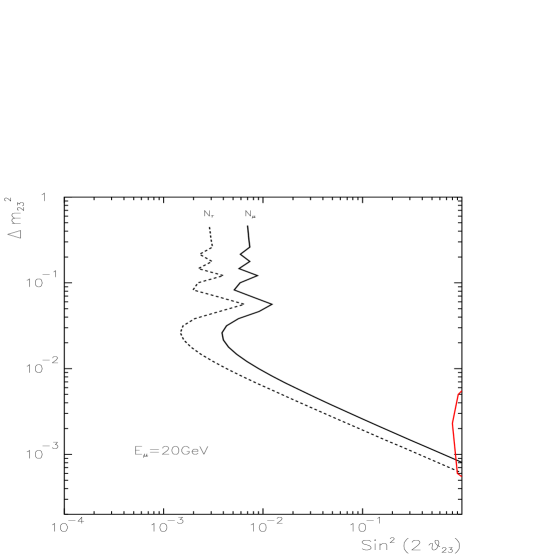
Figure 1: Sensitivity reach in the [$\sin^{2}(2\theta_{23}),\Delta m_{23}^{2}$] plane, at 90% confidence, for our reference beam and detectors and $L=732$ km. Continuous (dashed) boundaries correspond to $\mu$ disappearance ($\tau$ appearance). The small region close to $\sin^{2}(2\theta_{23})=1$ is the SuperK domain.

To study the oscillatory signal of the two-family scenario of Eq.(2) there is no advantage in measuring the charges of the produced charged leptons: for a stored $\mu^{-}$ beam one expects charged current neutrino interactions leading to positrons and negatively charged heavier leptons, as in Eq.(2). For Majorana neutrinos this is not strictly correct, but the specific wrong-sign and CP-violating effects are suppressed by an unsurmontable factor $m_{\nu}/E_{\nu}$. In a three-neutrino mixing scenario, contrarywise, measuring charges could be extremely useful and CP-violation effects are not suppressed by the mentioned factor.

3 Three-family mixing.

The mixing between $\nu_{e}$, $\nu_{\mu}$ and $\nu_{\tau}$ is described by a conventional Kobayashi-Maskawa matrix $V$ relating flavour to mass eigenstates (we are assuming throughout this note that neutrino fluctuat nec mergitur: there are no transitions to sterile neutrinos). For Dirac neutrinos and in an obvious notation:

$$\left(\matrix{\nu_{e}\cr\nu_{\mu}\cr\nu_{\tau}}\right)=\left(\matrix{c_{12}c_{13}&c_{13}s_{12}&s_{13}\cr-c_{23}s_{12}e^{i\delta}-c_{12}s_{13}s_{23}&c_{12}c_{23}e^{i\delta}-s_{12}s_{13}s_{23}&c_{13}s_{23}\cr s_{23}s_{12}e^{i\delta}-c_{12}c_{23}s_{13}&-c_{12}s_{23}e^{i\delta}-c_{23}s_{12}s_{13}&c_{13}c_{23}\cr}\right)\left(\matrix{\nu_{1}\cr\nu_{2}\cr\nu_{3}}\right).$$ (6)

Without loss of generality, we choose the convention in which all Euler angles lie in the first quadrant: $0<\theta_{ij}<\pi/2$, while the CP-phase is unrestricted: $0<\delta<2\,\pi$. Define

$$W_{\alpha\beta}^{jk}\equiv\,[V_{\alpha j}V_{\beta j}^{*}V_{\alpha k}^{*}V_{\beta k}]$$ (7)

and

$$\Delta_{jk}\equiv\frac{\Delta m_{jk}^{2}}{2\,E_{\nu}}\;.$$ (8)

The transition probabilities between different flavours are:

$$P(\nu_{\alpha}\rightarrow\nu_{\beta})\,=\,-4\;\sum_{k>j}\,{\rm Re}[W_{\alpha\beta}^{jk}]\,\sin^{2}\left({\Delta_{jk}\,L\over 2}\right)\,\pm\,2\,\sum_{k>j}\,{\rm Im}[W_{\alpha\beta}^{jk}]\,\sin(\Delta_{jk}\,L)$$ (9)

with the plus (minus) sign referring to neutrinos (antineutrinos).

Let us adopt, from solar and atmospheric experiments, the indication that $|\Delta m_{12}^{2}|\ll|\Delta m_{23}^{2}|$, that Barbieri et al. [15] have dubbed the “minimal scheme”. Though this mass hierarchy may not be convincingly established, the minimal scheme suffices for our purpose of delineating the main capabilities of a $\nu$ factory (we have to deviate from minimality only in the discussion of CP violation).

The difference between neutrino propagation in vacuum and in matter turns out not to have an important effect on the sensitivity limits that we discuss in this chapter (for a fixed baseline of $732$ km). They are relevant at larger distances. We postpone their discussion to the next chapter, though the figures introduced anon do take the matter effects into account.

Atmospheric or terrestrial experiments have an energy range such that $\Delta m^{2}\,L/E_{\nu}\ll 1$ for the smaller ($\Delta m_{12}^{2}$) but not necessarily for the larger ($\Delta m_{23}^{2}$) of these mass gaps. Even then, solar and atmospheric (or terrestrial) experiments are not (provided $\theta_{13}\neq 0$) two separate two-generation mixing effects. In the minimal scheme solar effects are accurately described by three parameters ($\theta_{12}$, $\Delta m_{12}^{2}$ and $\theta_{13}$), while the terrestrial effects of interest here depend on $\theta_{23}$, $\Delta m_{23}^{2}$ and $\theta_{13}$:

$$P(\nu_{e}\rightarrow\nu_{\mu}) = \sin^{2}(\theta_{23})\,\sin^{2}(2\theta_{13})\,\sin^{2}\left({\Delta_{23}\,L\over 2}\right)$$ (10)

$$P(\nu_{e}\rightarrow\nu_{\tau}) = \cos^{2}(\theta_{23})\,\sin^{2}(2\theta_{13})\,\sin^{2}\left({\Delta_{23}\,L\over 2}\right)$$ (11)

$$P(\nu_{\mu}\rightarrow\nu_{\tau}) = \cos^{4}(\theta_{13})\,\sin^{2}(2\theta_{23})\,\sin^{2}\left({\Delta_{23}\,L\over 2}\right)\;.$$ (12)

In the minimal scheme CP and T violation effects can be neglected, so that $P(\bar{\nu}_{\alpha}\to\bar{\nu}_{\beta})=P(\nu_{\alpha}\to\nu_{\beta})$ and $P(\nu_{\beta}\to\nu_{\alpha})=P(\nu_{\alpha}\to\nu_{\beta})$. With this information, Eqs.(12) and unitarity one can construct all relevant oscillation amplitudes, e.g. $P(\nu_{\mu}\to\nu_{\mu})$.

The approximate analysis of the SuperK data by Barbieri et al. [15] results (for the range of $\Delta m_{23}^{2}$ advocated by the SuperK collaboration) in the restrictions $\theta_{23}=45\pm 15^{o}$ and $\theta_{13}\sim 0\div 45^{o}$, with a preferred value around 13^o. Fogli et al. conclude [16], after a more thorough analysis and with equal confidence, that $\theta_{13}<23^{0}$, while their range of $\Delta m_{23}^{2}$ is a little narrower than the one obtained by the SuperK team [1]. We shall present results for the range of angles advocated in [15] and the range of masses of [1], simply because they are the widest.

All mixing probabilities in Eq.(12) have the same sinusoidal dependence on $\Delta m^{2}_{23}\,L/E_{\nu}$, entering into the description of a plethora of channels:

$$\mu^{-}\rightarrow e^{-}\, \nu_{\mu} \,\bar{\nu}_{e}\,;$$ (13)

$$\bar{\nu}_{e}\rightarrow\bar{\nu}_{e}\rightarrow e^{+}\;\;{\rm disappearance,}$$

$$\bar{\nu}_{e}\rightarrow\bar{\nu}_{\mu}\rightarrow\mu^{+}\;\;{\rm appearance,}$$

$$\bar{\nu}_{e}\rightarrow\bar{\nu}_{\tau}\rightarrow\tau^{+}\;\;{\rm appearance}\;\;\;(\tau^{+}\rightarrow\mu^{+};\;e^{+})\,,$$

$$\nu_{\mu} \rightarrow\nu_{\mu}\rightarrow\mu^{-}\;\;\;\;\;{\rm disappearance,}$$

$$\nu_{\mu} \rightarrow\nu_{e}\rightarrow e^{-}\;\;\;\;\;{\rm appearance,}$$

$$\nu_{\mu} \rightarrow\nu_{\tau}\rightarrow\tau^{-}\;\;\;\;\;{\rm appearance}\;\;\;(\tau^{-}\rightarrow\mu^{-};\,e^{-})\,.$$

The wrong sign channels of $\mu^{+}$, $\tau^{+}$ and $e^{-}$ appearance are the good news, relative to the two-generation analysis of Eqs.(2).

We extract results on the sensitivity to oscillations from observable numbers of muons, and not from ratios such as the number of muons upon the number of electrons, that are so useful in the analysis of atmospheric neutrinos. Our conclusions would be essentially identical, were we to draw them from the customary ratios. Yet, we refer directly to muon numbers not only because the neutrino-factory flux would be very well understood (obviating the main reason to take ratios), but also because the physics of three-generation mixing leads us to advocate the advantages of an experiment capable of measuring the charge of muons. It is likely that a relatively large experiment of this kind would compromise the possibility of efficiently distinguishing electron- from neutral-current events. Naturally, a complementary experiment on the same beam, capable of observing electrons with precision, would be useful [17, 18].

In Fig. 2 we show the sensitivity reach, in the [$\sin^{2}(\theta_{23}),\Delta m_{23}^{2}$] plane for various values of $\theta_{13}$, for $L=732$ km, for our reference set-up and for stored $\mu^{-}$s. We have chosen to illustrate the disappearance observable $N_{\mu}\equiv N[\mu^{+}+\mu^{-}]$ and the appearance measurement $N[\mu^{+}]$ (the effects of the small $\mu^{+}$ contamination from $\bar{\nu}_{e}\to\bar{\nu}_{\tau}$ oscillations, $\tau^{+}$ production and $\tau^{+}\to\mu^{+}$ decay, are negligible). Figure 2 conveys an important point: for stored $\mu^{-}$s the observation of $\mu^{+}$ appearance is very superior to a measurement (such as the depletion of the total number of muons) in which the charges of the produced leptons are not measured. This is true for all $\theta_{13}$ bigger than a few degrees. This angle is very unconstrained by current measurements. Notice that the SuperK domain would be covered for any $\sin^{2}(\theta_{13})>3.6\times 10^{-3}$ by the appearance channel, while the disappearance measurement would fall short of this motivating goal. All these statements refer to statistical sensitivities, in the absence of the backgrounds discussed in Section 6.

Fig. 1 and its comparison with Fig. 2 convey our point regarding the benefits of muon-charge identification. We are showing results only for stored $\mu^{-}$s. The wrong-sign muon results are slightly superior for the polarity we do not show: if it is positive, and for equal numbers of decays, the unoscillated numbers of expected electron events (and of potential wrong-sign muons) are roughly twice as numerous. The $\mu$-disappearance results, on the other hand, are slightly weaker for a $\mu^{+}$ beam.

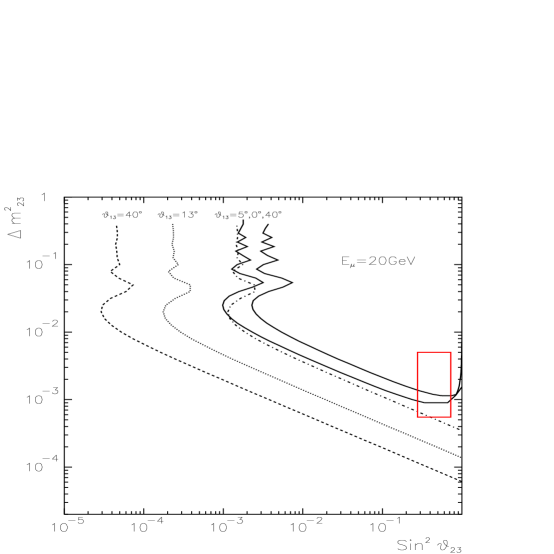
Figure 2: Sensitivity reach in the plane $[\sin^{2}\theta_{23},\Delta m_{23}^{2}]$ at 90% confidence, for our reference set-up, a $\mu^{-}$-decay beam and $L=732$ km. Matter effects are taken into account. The discontinuous lines correspond to the appearance observable $N[\mu^{+}]$ (at $\theta_{13}=40,13,5^{0}$) and the full lines correspond to the disappearance observable $N_{\mu}$ at $\theta_{13}=0,40^{0}$. The rectangle is the approximate domain allowed by SuperK data.

In Fig. 3 we show the sensitivity reach, in the [$\sin^{2}(\theta_{13}),\Delta m_{23}^{2}$] plane for the extremal values of $\theta_{23}\sim 30^{0},\,45^{0}$ allowed by the SuperK data. In Fig. 4 we show the sensitivity reach in the plane $[\sin^{2}\theta_{23},\sin^{2}\theta_{13}]$.

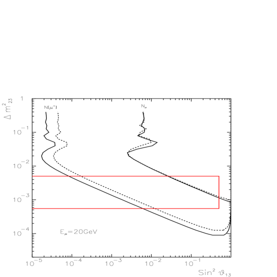
Figure 3: Sensitivity reach in the plane $[\sin^{2}\theta_{13},\Delta m_{23}^{2}]$, at 90% confidence, for the same conditions as in Fig. 2. The continuous (dashed) lines correspond to $\theta_{23}=45^{0}\,(30^{0})$. The lines covering the most (least) ground are for the appearance (disappearance) observable $N[\mu^{+}]$ ($N_{\mu}$). The rectangular domain is the approximate region allowed by SuperK data.

The overall conclusion of this analysis in terms of the mixing of three generations is that the capability of detecting “wrong-charge” muons would be extremely useful in giving access to the study of a large region of the ($\theta_{13}$, $\theta_{23}$, $\Delta m_{23}^{2}$) parameter space.

Figure 4: Sensitivity reach in the [$\sin^{2}\theta_{23},\sin^{2}\theta_{12}$] plane at 90% confidence, for the same conditions as in Fig. 2. The dashed and dotted lines correspond to the appearance observable $N[\mu^{+}]$ with $\Delta m_{23}^{2}=2\times 10^{-3}$ eV², and $\Delta m_{23}^{2}=10^{-3}$ eV², respectively. The regions interior to the continuous and dot-dashed lines are exclusion domains stemming from the disappearance observable, $N_{\mu}$, with $\Delta m_{23}^{2}=2\times 10^{-3}$ eV², and $\Delta m_{23}^{2}=10^{-3}$ eV², respectively.

4 Matter effects and scaling laws

Of all neutrino species, only $\nu_{e}$ and $\bar{\nu}_{e}$ have charged-current elastic scattering amplitudes on electrons. This, it is well known, induces effective “masses” $\mu=\pm\,2\,E_{\nu}\,A$, where the signs refer to $\nu_{e}$ and $\bar{\nu}_{e}$ and $A=\sqrt{2}\,G_{F}\,n_{e}$, with $n_{e}$ the ambient electron number density [5]. Matter effects [5, 20] are important if $A$ is comparable to, or bigger than, the quantity $\Delta_{jk}=\Delta m_{jk}^{2}/(2\,E_{\nu})$ of Eq.(8) for some mass difference and neutrino energy. In the minimal scheme $\Delta m_{12}^{2}$ is neglected relative to $\Delta m_{23}^{2}$, the question is the relative size of $A$ and $\Delta_{23}\simeq\Delta_{13}$ (we assume $\Delta m_{23}=m_{3}^{2}-m_{2}^{2}$ to be positive, otherwise the roles of neutrinos and antineutrinos are to be inverted in what follows).

For the Earth’s crust, with density $\rho\sim 2.8$ g/cm³ and roughly equal numbers of protons, neutrons and electrons, $A\sim 10^{-13}$ eV. The typical neutrino energies we are considering are tens of GeVs. For $E_{\nu}=12$ GeV (the average $\bar{\nu}_{e}$ energy in the decay of $E_{\mu}=20$ GeV muons) $A\simeq\Delta_{23}$ for $\Delta m^{2}_{23}=2.4\times 10^{-3}$ eV². This means that $A\gg\Delta_{23}$ for the lower $\Delta m^{2}$ values in Figs. 2,3 while the opposite is true at the other end of the relevant mass domain. Thus, the matter effects that we have so far neglected are dominant in the most relevant portion of the domain of interest: the lower mass scales. Yet, as we proceed to show, matter effects are practically irrelevant (except in the analysis of CP-violation effects) in long baseline experiments with $L<3000$ km. They only begin to have a sizeable impact at even larger distances.

Define

$$B\equiv\sqrt{\left[\Delta_{23}\,\cos(2\theta_{13})-A\right]^{2}+\left[\Delta_{23}\,\sin(2\theta_{13})\right]^{2}}$$ (14)

and

$$\sin(2\,\theta_{M})\equiv{\Delta_{23}\,\sin(2\theta_{13})/B}\,,$$ (15)

where $\theta_{M}$ is to be taken in the first (second) quadrant if $\Delta_{23}\,\cos(2\theta_{13})-A$ is positive (negative). The transition probability governing the appearance of wrong sign muons is, in the minimal scheme, in the presence of matter effects, and in the approximation of constant $n_{e}$ [21]:

$$P(\nu_{e}\rightarrow\nu_{\mu})\simeq s^{2}_{23}\,\sin^{2}(2\theta_{M})\,\sin^{2}\left({B\,L/2}\right)$$ (16)

which, for $A=0$, reduces to the corresponding vacuum result: the first of Eqs.(12). For $B\,L/2$ sufficiently small, it is a good approximation to expand the last sine in Eq.(16) and to use Eq.(15) to obtain:

$$P(\nu_{e}\rightarrow\nu_{\mu})\sim s^{2}_{23}\,\sin^{2}(2\theta_{13})\,\left[\Delta_{23}\,L/2\right]^{2}\,,$$ (17)

which coincides with the expansion for small $\Delta_{23}\,L/2=\Delta m^{2}_{23}\,L/(4\,E_{\nu})$ of the vacuum result in Eqs.(12), even when matter dominates and $B\simeq A$ (at a distance of $L=732$ km, $A\,L/2\sim 0.2$).

In practice, and after integration over the neutrino flux and cross section, the above approximations are excellent in that part of the disappearance sensitivity contours of Figs. 2-4 that are roughly “straight diagonal” lines of slope $-1$. There, $s_{23}\,\sin(2\theta_{13})\,\Delta m^{2}_{23}$ is approximately constant. In this region the results with and without matter effects are indistinguishable and (for equal number of events) the sensitivity contours from $\nu_{e}\to\nu_{\mu}$ and $\bar{\nu}_{e}\to\bar{\nu}_{\mu}$ transitions would also coincide.

For sufficiently large $\Delta m^{2}_{23}$, matter effects are negligible. In Figs. 2,3 this occurs in the portion of the limits that are approximately “straight vertical” lines, for which the oscillating factors in Eqs.(16,17) average to 1/2. All in all, only the wiggly regions in the sensitivity boundaries distinguish matter from vacuum, neutrinos from antineutrinos. The differences are not large (factors of order two). All of the above also applies to the disappearance-channel results shown in the same figures.

The preceding discussion was made in the context of the relatively “short” long baseline of 732 km and for $E_{\mu}=20$ GeV. How do our results scale to other distances and stored-muon energies? (the scaling laws differ somewhat from similar ones for neutrinos from $\pi$ and $K$ decay).

We are considering detectors at a sufficiently long distance (or otherwise sufficiently small in transverse dimensions) for the neutrino beam that bathes them to be transversally uniform. For a fixed number of decaying muons (independent of $E_{\mu}$) the forward neutrino flux varies as $E_{\mu}^{2}\,L^{-2}$, see Eq.(5). The neutrino cross sections at moderate energy are roughly linear in the neutrino (or parent-muon) energy. For $L<3000$ km, $\sin^{2}(A\,L/2)\sim(A\,L/2)^{2}$ is a good approximation (better than 25% and rapidly deteriorating for increasing $L$) and the vacuum-like result of Eq.(17) is applicable. Entirely analogous considerations apply to the probability $P(\nu_{\mu}\to\nu_{\mu})$ whose explicit form in the minimum scheme [21] we have not written. All this implies that the “straight diagonal” parts of the appearance contours in Figs. 2-4 scale as $s_{23}\,\sin(2\theta_{13})\,\Delta m^{2}_{23}\propto E_{\mu}^{-1/2}$, with no $L$ dependence. For $L>3000$ km, this sensitivity (still in the approximation of constant $n_{e}$) is weakened by an extra $L$-dependent factor so that, for any distance, the appearance sensitivity at the low-mass end scales as:

$$s_{23}\,\sin(2\theta_{13})\,\Delta m^{2}_{23}\propto E_{\mu}^{-1/2}\;(A\,L/2)/\big{|}\sin(A\,L/2)\big{|}\;.$$ (18)

For the “straight vertical” parts of the appearance boundaries in Figs. 2,3 the oscillation probabilities average to 50% and the scaling law is $s_{23}\,\sin(2\theta_{13})\propto L\,E_{\mu}^{-3/2}$.

For a disappearance channel the putative signal must compete with the statistical uncertainty in the background and the $E_{\mu}$ and $L$ dependence are not those of an appearance channel. Moreover, the scaling laws for our $N[\mu^{+}+\mu^{-}]$ contours are not very simple functions of the mixing angles. For $L<3000$ km their “straight diagonal” portions in Figs. 2,3 scale up and down as $\Delta m^{2}\propto E_{\mu}^{1/4}\,L^{-1/2}$. The “straight vertical” parts of these limits move right and left as $\sin\theta\propto L^{1/2}\,E_{\mu}^{-3/4}$. For $L>3000$ km the scaling laws for disappearance are more involved.

In Fig. 5 we compare results for $L=732$ and 6000 km. Only the disappearance channel at large $\sin^{2}\theta$ benefits from the larger distance. For the more attractive wrong-sign $\mu$-appearance channel there is no advantage to a very long baseline.

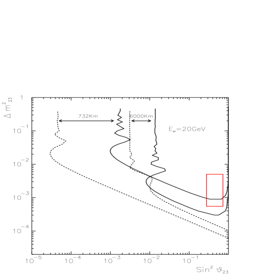
Figure 5: Sensitivity reach in the plane $[\sin^{2}\theta_{23},\Delta m_{23}^{2}]$ at 90% confidence, for our reference set-up, a $\mu^{-}$-decay beam and $L=732,\,6000$ km. The discontinuous (continuous) lines correspond to the appearance (disappearance) observable $N[\mu^{+}]$ ($N[\mu^{+}+\mu^{-}]$). We chose $\theta_{13}=40^{0}$ for appearance, $\theta_{13}=0$ for disappearance.

5 T and CP violation ?

The beams from a hypothetical neutrino factory would be so intense and well understood that one may daydream about measuring CP violation in the very clean environment of a $\mu$-decay beam. Standard-model CP-violation effects, as is well known in the quark sector, entail an unavoidable reference to all three families. They would consequently vanish in the minimal scheme that we have been considering, insofar as the mass difference $\Delta m^{2}_{12}$ is neglected. With the inclusion of this difference the parameter space (two mass gaps, three angles, one CP-odd phase) becomes so large that its conscientious exploration would, in our current nescient state, be premature. We will simply give some examples of the size of the effects that one could, rather optimistically, expect.

CP-related observables often involve the comparison between measurements in the two charge-conjugate modes of the factory. One example is the asymmetry [22]

$$A_{e\mu}^{CP}\equiv\frac{P(\nu_{e}\rightarrow\nu_{\mu})-P(\bar{\nu}_{e}\rightarrow\bar{\nu}_{\mu})}{P(\nu_{e}\rightarrow\nu_{\mu})+P(\bar{\nu}_{e}\rightarrow\bar{\nu}_{\mu})}\,$$ (19)

which would, in vacuum, be a CP-odd observable. The voyage through our CP-uneven planet, however, induces a non-zero $A_{e\mu}^{CP}$ even if CP is conserved, since $\nu_{e}$ and $\bar{\nu}_{e}$ are differently affected by the ambient electrons [23].

In a neutrino factory $A_{e\mu}^{CP}$ would be measured by first extracting $P(\nu_{\mu}\rightarrow\nu_{e})$ from the produced (wrong-sign) $\mu^{-}$s in a beam from $\mu^{+}$ decay and $P(\bar{\nu}_{e}\rightarrow\bar{\nu}_{\mu})$ from the charge conjugate beam and process. Even if the fluxes are very well known, this requires a good knowledge of the cross section ratio $\sigma(\bar{\nu}_{\mu}\to\mu^{+})/\sigma(\nu_{\mu}\to\mu^{-})$, which may be gathered in a short-baseline experiment. To obtain the genuinely CP-odd quantity of interest, the matter effects must be subtracted with sufficient precision. But we shall see that the truly serious limitation is the small statistics inherent to appearance channels.

The T-odd asymmetry [24]

$$A_{e\mu}^{T}\equiv\frac{P(\nu_{e}\rightarrow\nu_{\mu})-P(\nu_{\mu}\rightarrow\nu_{e})}{P(\nu_{e}\rightarrow\nu_{\mu})+P(\nu_{\mu}\rightarrow\nu_{e})}\;$$ (20)

is “cleaner” than the CP-odd one, in that a non-zero value for it cannot be induced by matter effects. As a consequence of CPT-invariance the two asymmetries, in vacuum, are identical $A_{e\mu}^{T}[{\rm vac}]=A_{e\mu}^{CP}[{\rm vac}]$. The $T$-odd asymmetry is very difficult to measure in practice. In a $\mu^{-}$-generated beam the extraction of $P(\nu_{\mu}\rightarrow\nu_{e})$ would require a measurement of electron charge, the $e^{+}+e^{-}$ number involving also $P(\bar{\nu}_{e}\rightarrow\bar{\nu}_{e})$. It is not easy to measure the electron charge in a large, high-density experiment.

The complete expressions for $A^{CP}_{e\mu}$ in the presence of matter are rather elaborate and we do not reproduce them here. To illustrate the size of the effects, in Table 1 we give the values of various asymmetries at $L=732$ km with a fixed neutrino energy, $E_{\nu}=7$ GeV with maximal CP violation, $\delta=90^{0}$, and with various parameter values chosen in their currently allowed domains. The Table reports the vacuum asymmetry $A^{CP}_{e\mu}[{\rm vac}]$, the calculated expectation $A^{CP}_{e\mu}(0)$ for the apparent CP-odd asymmetry induced by matter, and the genuine CP-odd asymmetry in matter:

$${{\cal A}_{e\mu}}(\delta)=A^{CP}_{e\mu}(\delta)-A^{CP}_{e\mu}(0)\;,$$ (21)

in which the matter effect is subtracted.

$\sin^{2}\theta_{12}$ $\theta_{13}$ $\Delta m^{2}_{12}$ $A^{CP}_{e\mu}[{\rm vac}]$ ${\cal A}_{e\mu}$ $A^{CP}_{e\mu}(0)$ 0.5 13⁰ $10^{-5}$ $-5.9\,10^{-3}$ $-5.5\,10^{-3}$ $1.6\,10^{-2}$ $5\,10^{-3}$ 30⁰ $10^{-4}$ $-3.4\,10^{-3}$ $-3.2\,10^{-3}$ 9.8 $10^{-3}$ 0.5 30⁰ $10^{-4}$ $-2.6\,10^{-2}$ $-2.5\,10^{-2}$ $7.8\,10^{-3}$ 0.5 13⁰ $10^{-4}$ $-5.6\,10^{-2}$ $-5.4\,10^{-2}$ $1.4\,10^{-2}$

Table 1: The CP asymmetries defined in the text, at $L=732$ km, for $\delta=\pi/2$, $\theta_{23}=45^{0}$, $\Delta m^{2}_{23}=10^{-3}$ eV², $E_{\nu}=7$ GeV and choices of other parameters compatible with solar and atmospheric data.

With no further ado, Table 1 conveys the message that, if $\Delta m^{2}_{21}$ is indeed as small as the ensemble of solar neutrino experiments would imply, the CP-odd effects are only sizeable in a small domain of parameter space, exemplified here by the last two rows of the table. Is that region amenable to empiric scrutiny?

A first question concerns the relative size of the measured and the theoretically subtracted terms. For the subtraction procedure to be useful $\theta_{23}$, $\theta_{13}$, $\Delta m^{2}_{23}$ and the density profile traversed by the beam must be known with sufficient precision for the error in the subtracted term not to dominate the result. At the distance of $L=732$ km used to construct Table 1, this does not seem to be a problem: for the parameter values of the last two rows, the subtractions are small enough that a precision of a factor of two in their determination would suffice.

A second question on the observability of CP-violation is that of statistics. In practice, for our reference set-up, there would be too few events to exploit the explicit $E_{\nu}$ dependence of the CP-odd effect. To construct a realistic CP-odd observable, consider the neutrino-energy integrated quantity:

$${\bar{A}}^{CP}_{e\mu}=\frac{\large\{{N[\mu^{-}]}/{N_{o}[e^{-}]}\large\}_{+}-\large\{N[\mu^{+}]/N_{o}[e^{+}]\large\}_{-}}{\large\{N[\mu^{-}]/N_{o}[e^{-}]\large\}_{+}+\large\{N[\mu^{+}]/N_{o}[e^{+}]\large\}_{-}}\;,$$ (22)

where the sign of the decaying muons is indicated by a subindex, $N[\mu^{+}]$ $(N[\mu^{-}])$ are the measured number of wrong-sign muons, and $N_{o}[e^{+}]$ $(N_{o}[e^{-}])$ are the expected number of $\bar{\nu}_{e}(\nu_{e})$ charged current interactions in the absence of oscillations. The genuine CP-odd asymmetry is ${\overline{\cal A}}_{e\mu}(\delta)=\bar{A}_{e\mu}^{CP}(\delta)-\bar{A}_{e\mu}^{CP}(0)$, the flux and cross-section weighed version of Eq.(21).

In Fig. 6 we give the signal over statistical noise ratio for $\big{|}{\overline{\cal A}}_{e\mu}(\pm\pi/2)\big{|}$ as a function of distance for our standard set-up, for $E_{\mu}=10,20$ GeV and for the parameters in the last row of Table 1. The number of “standard deviations” is seen not to exceed $\sim 2$ at any distance. Moreover, for very long baselines, the relative size of the theoretically subtracted term $\bar{A}_{e\mu}^{CP}(0)$ increases very rapidly, as shown in Fig. 7. We have examined other parameter values within the limits of the scenario we have adopted for neutrino masses and mixing angles. As an example, increasing $\Delta m^{2}_{23}$ from $10^{-3}$ to $6\times 10^{-3}$ eV², with the other parameters fixed as in Table 1, increases the maximum number of standard deviations to $\sim 3.5$ (at $L\sim 3000$ km) but the relative size of the theoretically subtracted term at that distance increases by an order of magnitude relative to what it is in Fig. 7.

The conclusion is that, if the neutrino mass differences are those indicated by solar and atmospheric observations and the physics is that of three standard families, there is little hope to observe CP-violation with the beams and detectors we have described.

Figure 6: Signal over statistical uncertainty in a measurement of CP asymmetries as a function of distance, with the continuous (dashed) lines corresponding to $E_{\mu}=20\,(10)$ GeV. The chosen CKM parameters are those of the last row of Table 1. The lower four curves describe $\big{|}{\overline{\cal A}}_{e\mu}(\pm\pi/2)\big{|}$ over its statistical error. The upper two curves are vacuum results for the same CP phase(s).

Figure 7: Ratio of the subtracted term $\bar{A}_{e\mu}^{CP}(0)$ relative to the genuine CP asymmetry ${\overline{\cal A}}_{e\mu}(\pi/2)$, as a function of distance, with the continuous (dashed) lines corresponding to $E_{\mu}=20\,(10)$ GeV. The chosen CKM parameters, are those of the last row of Table 1.

6 Observables and backgrounds in $\pi$- and $\mu$-decay beams.

In a search for $\tau$ appearance, a $\mu$-decay beam, but for its conceivable intensity, would not have overwhelming advantages relative to a conventional $\pi+K$ decay beam; the contamination of $\nu_{\tau}$ from $D_{s}$ decay in the $\pi$ beam is known to be small, witness the fact that the third generation neutrino has not yet been “seen”. The background from the charmed particles produced by the other neutrino types would be equally challenging in a conventional or a $\nu$-factory beam. We briefly compare these beams for oscillation studies other than $\tau$ appearance.

The $\nu_{\mu}$ beams from $\pi$ decay have a contamination of $\nu_{e}$s from $K_{e3}$ decays. A small contamination of the wrong helicity neutrinos (e.g. $\bar{\nu}_{\mu}$ in a predominantly $\nu_{\mu}$ beam) is also unavoidable, due to limitations of the charge-separation and focusing system. It is difficult to understand these beams theoretically to better than 10% precision. With a $\pi^{+}$ decay beam one can measure neutral currents and the production of electrons and muons, the measurement of whose charge is immaterial; that is, a total of three observables, one of which (electron events) is beset by background problems. Ideally beams of opposite polarity add information, but the comparison of $\nu_{\mu}$ and $\bar{\nu}_{\mu}$ disappearance channels for a study of CP-violation would be even more demanding than for the $\nu$-factory wrong-sign $\mu$-appearance examples discussed in the previous section.

The number of useful observables in an experiment with a $\nu_{\mu}+\bar{\nu}_{e}$ beam from $\mu^{-}$ decay is larger than for a $\pi$ decay beam. Assume that one or various aligned experiments are capable of distinguishing $\mu^{+}$, $\mu^{-}$, $e^{+}+e^{-}$, and neutral current events. One of these observables ($\mu^{+}$ appearance) is a tell-tale signal of oscillations. From the other three observables one can extract information on oscillation probabilities with errors associated only with statistics, backgrounds, efficiencies and cross sections, but with very small flux uncertainties. In total, for each polarity, a $\mu$-decay facility could measure four channels other than $\tau$ appearance. In principle this is sufficient to determine (or severely constrain) two of the three Euler angles ($\theta_{23}$ and $\theta_{13}$) of the neutrino-mixing matrix in Eq.(6) and (with a measurement of $E_{\nu}$) the neutrino mass splitting $\Delta m^{2}_{23}$. With a conventional $\pi$-decay beam such a program would be out of reach.

The backgrounds to a wrong-sign $\mu$ signal are not associated with the beam, but with the numerous decay processes that can produce or fake such muons. Pions masquerading as muons can be ranged out with great efficiency, particularly in competition with the generally energetic primary muon from the leptonic vertex. Muonic charged currents are not the most threatening background, since one would also have to miss the right-sign muon. Electronic charged currents may singly produce charmed particles, but the decays of the latter lead to muons of the “right” sign. In any case, the background from charm production and subsequent muonic decay can be easily suppressed or studied by lowering $E_{\mu}$ below the canonical 20 GeV we have been using. At 1/4 the stored muon energy the statistical appearance sensitivity would be reduced by a factor of 2, while charm production would be almost completely kinematically forbidden (this is an extreme example, in that it might jeopardize muon recognition). Neutral current events in which a hadron decays into a muon early or straight enough are presumably the main hazard. Experience with NOMAD –admittedly not a coarse-grained very large device– demonstrates that an ‘isolation’ cut in the transverse momentum of the muon candidate relative to the direction of the hadronic jet is extremely efficient [19]. In these events, an additional cut of the missing transverse momentum (carried mainly by the outgoing neutrino in the neutral-current leptonic vertex) relative to the muon plus hadrons would also help. Even detectors as coarse-grained as MINOS [3] or NICE [25] have jet-direction reconstruction capabilities and could implement similar cuts.

Without a specific detector in mind and considerable simulation toil we cannot answer the question of how large the above backgrounds would be. A question that we can answer is how small they would have to be not to interfere with the signal. For our standard set-up and an unoptimized $E_{\mu}=$ 20 GeV, there would be a grand total of a few $10^{5}$ events for $n_{\mu}=2\times 10^{20}$ $\mu$ decays at $L=732$ km. To compete with a limiting appearance signal of a few wrong-sign muons may be difficult. At some 10 times larger $L$ the low-mass edge of the sensitivity domain would change very little, as shown in Eq.(18) and Fig. 5, while the background would be reduced by two orders of magnitude, a level at which it would not represent a challenge. The overall optimization of the signal-to-noise ratio is a multi-parameter task that we cannot engage in.

7 Summary.

The inevitable conclusion of a description of atmospheric and solar neutrino data as two independent two-by-two neutrino-mixing effects is that the only hope to corroborate the atmospheric results with artificial beams is based on long baseline experiments looking for $\tau$ appearance or $\mu$ depletion. These experiments would have great difficulty in covering the parameter space favoured by SuperK. If the same data are analysed in a three-generation mixing scenario, the conclusions are very different: long baseline experiments searching for $\nu_{e}\leftrightarrow\nu_{\mu}$ transitions regain interest, since these oscillations (even if primarily responsible for the long-distance solar effect) will in general also occur over the shorter range implied by the atmospheric data.

We have studied $\nu_{\mu}\leftrightarrow\nu_{e}$ oscillations in the context of a neutrino factory. Rather than concentrating on the $\nu_{\mu}\to\nu_{\tau}$ process, the observation of which is notoriously difficult, we have outlined the possibilities opened by experiments searching, not only for an unexpected $e/\mu$ production ratio, but very preferably for the appearance of “wrong sign” muons: $\mu^{\pm}$s in a beam from decaying $\mu^{\mp}$s. We have not dealt in detail with the problem of backgrounds.

A neutrino factory may provide beams clean and intense enough, not only to corroborate the strong indication for neutrino oscillations gathered by the SuperK collaboration, but also to launch a program of precision neutrino-oscillation physics. The number of useful observables is sufficient to determine or very significantly constrain the parameters $\theta_{23}$ and $\theta_{13}$ and $\Delta m^{2}_{23}$ of a standard three-generation mixing scheme. Only if the neutrino mass differences are much larger than we have assumed would a neutrino factory serve to measure the remaining mixing parameters of the very clean neutrino-mixing sector.

It is instructive to compare the current programs to measure the CKM mixing matrices in the quark and lepton sectors. Considerable effort is being invested, sometimes in duplicate, to improve our knowledge of the quark sector case, mainly via better studies of $B$-decay. Even though non-zero neutrino masses are barely established, the neutrino sector of the theory can be convincingly argued to herald physics well beyond the standard model [26]. It is in this perspective –with dedicated $B$-physics experiments and beauty factories in the background– that a neutrino factory should be discussed.

All by itself, as part of a muon-collider complex or even as a step in its R&D, a neutrino factory seems to be a must.

8 Acknowledgements

We acknowledge useful conversations with B. Autin, L. Camilleri, L. Di Lella, J. Ellis, J. Gómez-Cadenas, O. Mena, P. Picchi, F. Pietropaolo, C. Quigg, J. Steinberger, P. Strolin and J. Terrón. M. B. G. thanks the CERN Theory Division for hospitality during the initial stage of this work; her work was partially supported as well by CICYT project AEN/97/1678.

References

- [1] Y. Fukuda et al., Phys. Lett. B433(1998) 9, hep-ex/9805006, Phys. Rev. Lett. 81 (1998) 1562; T. Kagita, in Proceedings of the XVIIIth International Conference on Neutrino Physics and Astrophysics, Takayama, Japan (June 1998).
- [2] Y. Fukuda et al., Phys. Lett. B335 (1994) 237.
- [3] E. Ables et al., MINOS Collaboration, Fermilab Proposal P-875 (1995).
- [4] G. Aquistapace et al., CERN 98-02, INFN/AE-98/05 (May 1998).
- [5] L. Wolfenstein, Phys. Rev. D17(1978) 2369; D20 (1979) 2634; S.P. Mikheyev and A. Yu Smirnov, Sov. J. Nucl. Phys. 42(1986) 913.
- [6] B. Pontecorvo, Sov. Phys. JETP 26, 984 (1968).
- [7] S. Geer, Phys. Rev D57 (1989) 6989.
- [8] B. Autin et al., CERN-SPSC/98-30, SPSC/M 617 (October 1998).
- [9] A. Ereditato, K. Niwa and P. Strolin, Proc. of Weak Interactions and Neutrino Workshop, Capri(1997), Nucl. Phys B Proc. Supplement 66 (1998) 423; H. Shibuya et al., OPERA Collaboration, CERN-SPSC 97-24, LNGS-LOI 8/97 (1997).
- [10] C. Athanassopoulos et al., Phys. Rev. Lett. 77(1996) 3082.
- [11] G.L. Fogli and E. Lisi, Phys. Rev. D 54 (1996) 3667.
- [12] See for example F. Boehm and P. Vogel, Physics of Massive Neutrinos, Cambridge University Press, 1997.
- [13] A. Bueno, M. Campanelli and A. Rubbia, hep-ph/9808485.
- [14] C.H. Albright and C. Jarlskog, Nucl. Phys. B84(1975) 467.
- [15] R. Barbieri et al., hep-ph/9807235, LBNL-42020, UCB-PTH-98/44, SNS-PH/98-15, IFUP-TH/98-25.
- [16] G.L. Fogli et al., hep-ph/9808205, BARI-TH-308-98.
- [17] The ICARUS project, C. Rubbia, Nucl. Phys. Proc. Suppl. 48 (1996) 172.
- [18] T. Ypsilantis et al., AQUARICH, Nucl. Instrum. Methods A371 (1996) 330.
- [19] A. Bueno, M. Campanelli and A. Rubbia, hep-ph/9809252.
- [20] V. Barger et al., Phys. Rev. D22 (1980) 2718, H.W. Zaglauer and K.H. Schwarzer, Z. Phys. C 40 (1988) 273.
- [21] O. Yasuda, hep-ph/9809205, TMUP-HEL-9810.
- [22] N. Cabibbo, Phys. Lett. B72 (1978) 33.
- [23] J. Arafune, M. Koike and J. Sato, Phys. Rev. D 56 (1997) 3093, hep-ph/9703351. M. Tanimoto, Phys. Lett B 345 (1998) 373, hep-ph/9806375. H. Minakata and H. Nunokawa, Phys. Lett. B413 (1997) 369; Phys. Rev. D57 (1998) 4403.
- [24] T.K. Kuo and J. Pantalone, Phys. Lett. 198 B (1987) 406; S.M. Bilenky, C. Giunti and W. Grimus, hep-ph/9712537.
- [25] G. Baldini et al., NICE proposal, LNGS-LOI 98/13 (1998).
- [26] For a recent review, see Wilczcek in NEUTRINO 98, Takayama (Japan), June 1998, hep-ph/9809509, IASSNS-HEP-98-79.