ANOMALOUS HIGGS COUPLINGS AT COLLIDERS

I summarize our results on the attainable limits on the coefficients of dimension–6 operators from the analysis of Higgs boson phenomenology using data taken at Tevatron RUNI and LEPII. Our results show that the coefficients of Higgs–vector boson couplings can be determined with unprecedented accuracy. Assuming that the coefficients of all “blind” operators are of the same magnitude, we are also able to impose bounds on the anomalous vector–boson triple couplings comparable to those from double gauge boson production at the Tevatron and LEPII

.

1 Introduction

Despite the impressive agreement of the Standard Model (SM) predictions for the fermion–vector boson couplings with the experimental results, the couplings among the gauge bosons are not determined with the same accuracy. The $SU_{L}(2)\times U_{Y}(1)$ gauge structure of the model completely determines these self–couplings, and any deviation can indicate the existence of new physics beyond the SM.

Effective Lagrangians are useful to describe and explore the consequences of new physics in the bosonic sector of the SM $\!{}^{{\bf?},{\bf?},{\bf?},{\bf?}}$. After integrating out the heavy degrees of freedom, anomalous effective operators can represent the residual interactions between the light states. Searches for deviations on the couplings $WWV$ ($V=\gamma,Z$) have been carried out at different colliders and recent results $\!{}^{{\bf?}}$ include the ones by CDF $\!{}^{{\bf?}}$, and DØ Collaborations $\!{}^{{\bf?},{\bf?}}$. Forthcoming perspectives on this search at LEP II CERN Collider $\!{}^{{\bf?},{\bf?}}$, and at upgraded Tevatron Collider $\!{}^{{\bf?}}$ were also reported.

In the framework of effective Lagrangians respecting the local $SU_{L}(2)\times U_{Y}(1)$ symmetry linearly realized, the modifications of the couplings of the Higgs field ($H$) to the vector gauge bosons ($V$) are related to the anomalous triple vector boson vertex $\!{}^{{\bf?},{\bf?},{\bf?},{\bf?}}$. Here, I summarize our results on the attainable limits on the coefficients of dimension–6 operators from the analysis of Higgs boson phenomenology using data taken at Tevatron RUNI and LEPII. Our results show that the coefficients of Higgs–vector boson couplings can be determined with unprecedented accuracy. Assuming that the coefficients of all “blind” operators are of the same magnitude, we are also able to impose bounds on the anomalous vector–boson triple couplings comparable to those from double gauge boson production at the Tevatron and LEPII.

2 Effective Lagrangians

A general set of dimension–6 operators that involve gauge bosons and the Higgs scalar field, respecting local $SU_{L}(2)\times U_{Y}(1)$ symmetry, and $C$ and $P$ conserving, contains eleven operators $\!{}^{{\bf?},{\bf?}}$. Some of these operators either affect only the Higgs self–interactions or contribute to the gauge boson two–point functions at tree level and can be strongly constrained from low energy physics below the present sensitivity of high energy experiments $\!{}^{{\bf?},{\bf?}}$. The remaining five “blind” operators can be written as $\!{}^{{\bf?},{\bf?},{\bf?}}$,

$${\cal L}_{\mbox{eff}}=\sum_{i}\frac{f_{i}}{\Lambda^{2}}{\cal O}_{i}=\frac{1}{\Lambda^{2}}\Bigl{[}f_{WWW}\,Tr[\hat{W}_{\mu\nu}\hat{W}^{\nu\rho}\hat{W}_{\rho}^{\mu}]$$

$$+f_{W}(D_{\mu}\Phi)^{\dagger}\hat{W}^{\mu\nu}(D_{\nu}\Phi)+f_{B}(D_{\mu}\Phi)^{\dagger}\hat{B}^{\mu\nu}(D_{\nu}\Phi)$$ (1)

$$+f_{WW}\Phi^{\dagger}\hat{W}_{\mu\nu}\hat{W}^{\mu\nu}\Phi+f_{BB}\Phi^{\dagger}\hat{B}_{\mu\nu}\hat{B}^{\mu\nu}\Phi\Bigr{]}$$

where $\Phi$ is the Higgs field doublet, and

$$\hat{B}_{\mu\nu}=i(g^{\prime}/2)B_{\mu\nu}\;\;\hat{W}_{\mu\nu}=i(g/2)\sigma^{a}W^{a}_{\mu\nu}$$

with $B_{\mu\nu}$ and $W^{a}_{\mu\nu}$ being the field strength tensors of the $U(1)$ and $SU(2)$ gauge fields respectively.

Anomalous $H\gamma\gamma$, $HZ\gamma$, and $HZZ$ and $HWW$ and couplings are generated by (1), which, in the unitary gauge, are given by

$${\cal L}_{\mbox{eff}}^{\mbox{H}} = g_{H\gamma\gamma}HA_{\mu\nu}A^{\mu\nu}+g^{(1)}_{HZ\gamma}A_{\mu\nu}Z^{\mu}\partial^{\nu}H$$ (2)

$$+ g^{(2)}_{HZ\gamma}HA_{\mu\nu}Z^{\mu\nu}+g^{(1)}_{HZZ}Z_{\mu\nu}Z^{\mu}\partial^{\nu}H$$

$$+ g^{(2)}_{HZZ}HZ_{\mu\nu}Z^{\mu\nu}+g^{(2)}_{HWW}HW^{+}_{\mu\nu}W_{-}^{\mu\nu}\;$$

$$+ g^{(1)}_{HWW}\left(W^{+}_{\mu\nu}W_{-}^{\mu}\partial^{\nu}H+h.c.\right)\,$$

where $A(Z)_{\mu\nu}=\partial_{\mu}A(Z)_{\nu}-\partial_{\nu}A(Z)_{\mu}$. The effective couplings $g_{H\gamma\gamma}$, $g^{(1,2)}_{HZ\gamma}$, and $g^{(1,2)}_{HZZ}$ and $g^{(1,2)}_{HWW}$ are related to the coefficients of the operators appearing in (1) through,

$$g_{H\gamma\gamma} = -\left(\frac{gM_{W}}{\Lambda^{2}}\right)\frac{s^{2}(f_{BB}+f_{WW})}{2}\;,$$

$$g^{(1)}_{HZ\gamma} = \left(\frac{gM_{W}}{\Lambda^{2}}\right)\frac{s(f_{W}-f_{B})}{2c}\;,$$

$$g^{(2)}_{HZ\gamma} = \left(\frac{gM_{W}}{\Lambda^{2}}\right)\frac{s[2s^{2}f_{BB}-2c^{2}f_{WW}]}{2c}\;,$$ (3)

$$g^{(1)}_{HZZ} = \left(\frac{gM_{W}}{\Lambda^{2}}\right)\frac{c^{2}f_{W}+s^{2}f_{B}}{2c^{2}}\;,$$

$$g^{(2)}_{HZZ} = -\left(\frac{gM_{W}}{\Lambda^{2}}\right)\frac{s^{4}f_{BB}+c^{4}f_{WW}}{2c^{2}}\;,$$

$$g^{(1)}_{HWW} = \left(\frac{gM_{W}}{\Lambda^{2}}\right)\frac{f_{W}}{2}\;,$$

$$g^{(2)}_{HWW} = -\left(\frac{gM_{W}}{\Lambda^{2}}\right)f_{WW}\;,$$

with $g$ being the electroweak coupling constant, and $s(c)\equiv\sin(\cos)\theta_{W}$.

Equation (1) also generates new contributions to the triple gauge boson vertex. Using the standard parametrization for the C and P conserving vertex $\!{}^{{\bf?}}$

$${\cal L}_{WWV} = g_{WWV}\Bigg{\{}g_{1}^{V}\Big{(}W^{+}_{\mu\nu}W^{-\,\mu}V^{\nu}-W^{+}_{\mu}V_{\nu}W^{-\,\mu\nu}\Big{)}$$ (4)

$$+ \kappa_{V}W_{\mu}^{+}W_{\nu}^{-}V^{\mu\nu}+\frac{\lambda_{V}}{M_{W}^{2}}W^{+}_{\mu\nu}W^{-\,\nu\rho}V_{\rho}^{\;\mu}\Bigg{\}}\;,$$

where $V=Z,\gamma$, the coupling constants are $g_{WW\gamma}=e$ and $g_{WWZ}=e/(s\,c)$. The field-strength tensors include only the Abelian parts, i.e. $W^{\mu\nu}=\partial^{\mu}W^{\nu}-\partial^{\nu}W^{\mu}$ and $V^{\mu\nu}=\partial^{\mu}V^{\nu}-\partial^{\nu}V^{\mu}$, and

$$g_{1}^{Z} = 1+\frac{1}{2}\frac{M_{Z}^{2}}{\Lambda^{2}}f_{W}\;,$$

$$\kappa_{\gamma} = 1+\frac{1}{2}\frac{M_{W}^{2}}{\Lambda^{2}}\Big{(}f_{W}+f_{B}\Big{)}\;,$$ (5)

$$\kappa_{Z} = 1+\frac{1}{2}\frac{M_{Z}^{2}}{\Lambda^{2}}\Big{(}c^{2}f_{W}-c^{2}f_{B}\Big{)}\;,$$

$$\lambda_{\gamma}=\lambda_{Z} = \frac{3}{2}s^{2}\frac{M_{W}^{2}}{\Lambda^{2}}f_{WWW}\;.$$ (6)

As seen above, the operators ${\cal O}_{W}$ and ${\cal O}_{B}$ give rise to both anomalous Higgs–gauge boson couplings and to new triple and quartic self–couplings amongst the gauge bosons, while the operator ${\cal O}_{WWW}$ solely modifies the gauge boson self–interactions. The operators ${\cal O}_{WW}$ and ${\cal O}_{BB}$ only affect $HVV$ couplings, like $HWW$, $HZZ$, $H\gamma\gamma$ and $HZ\gamma$, since their contribution to the $WW\gamma$ and $WWZ$ tree–point couplings can be completely absorbed in the redefinition of the SM fields and gauge couplings $\!{}^{{\bf?}}$. Therefore, one cannot obtain any constraint on these couplings from the study of anomalous trilinear gauge boson couplings.

3 New Higgs Signatures

In this talk I will review our results on Higgs production at the Fermilab Tevatron collider and at LEPII with its subsequent decay into two photons $\!{}^{{\bf?}}$. This channel in the SM occurs at one–loop level and it is quite small, but due to the new interactions (1), it can be enhanced and even become dominant. I will summarized our results on the signatures:

$$p\,\bar{p} \rightarrow j\,j\,\gamma\,\gamma$$

$$p\,\bar{p} \rightarrow \gamma\,\gamma\,+\,\not\!\!E_{T}$$

$$p\,\bar{p} \rightarrow \gamma\,\gamma\,\gamma$$ (7)

$$e^{+}\,e^{-} \rightarrow j\,j\,\gamma\,\gamma$$

$$e^{+}\,e^{-} \rightarrow \gamma\,\gamma\,\gamma$$

We have included in our calculations all SM (QCD plus electroweak), and anomalous contributions that lead to these final states. The SM one-loop contributions to the $H\gamma\gamma$ and $HZ\gamma$ vertices were introduced through the use of the effective operators with the corresponding form factors in the coupling $\!{}^{{\bf?}}$. Neither the narrow–width approximation for the Higgs boson contributions, nor the effective $W$ boson approximation were employed. We consistently included the effect of all interferences between the anomalous signature and the SM background. As an example of I quote here that 1928 SM amplitudes plus 236 anomalous ones, contribute to the process $p\,\bar{p}\rightarrow j\,j\,\gamma\,\gamma$ $\!{}^{{\bf?}}$. The SM Feynman diagrams corresponding to the background subprocess were generated by Madgraph $\!{}^{{\bf?}}$ in the framework of Helas $\!{}^{{\bf?}}$. The anomalous couplings arising from the Lagrangian (1) were implemented in Fortran routines and were included accordingly. For the $p\,\bar{p}$ processes, we have used the MRS (G) $\!{}^{{\bf?}}$ set of proton structure functions with the scale $Q^{2}=\hat{s}$.

All processes listed in (7) have been the object of direct experimental searches. In our analysis we have closely followed theses searches in order to make our study as realistic as possible. In particular when studying the $\gamma\gamma jj$ final state we have closely followed the results recently presented by DØ Collaboration for $p\bar{p}\rightarrow\gamma\gamma jj$ events with high two–photon invariant mass $\!{}^{{\bf?}}$.

For events containing two photons plus large missing transverse energy ($\gamma\gamma\not\!\!E_{T}$) as well as three photons in the final state we have used the results from DØ and CDF collaborations $\!{}^{{\bf?},{\bf?},{\bf?}}$. These events represent an important signature for some classes of supersymmetric models and in Refs.$\!{}^{{\bf?},{\bf?},{\bf?}}$ the experimental collaborations use their results to set limits in some of the SUSY parameters. However, as we pointed out $\!{}^{{\bf?}}$, these final states can also be a signal of Higgs production and subsequent decay into photons and can be used to place limits on the coefficients of the anomalous operators (1).

Finally, in order to obtain constraints on the anomalous couplings described above, we have also used the OPAL data $\!{}^{{\bf?},{\bf?}}$ for the reactions,

$$e^{+}e^{-} \rightarrow \gamma\gamma\gamma\;,$$ (8)

$$e^{+}e^{-} \rightarrow \gamma\gamma+\mbox{ hadrons}\;.$$ (9)

As an example, I describe below more in detail our analysis of the $\gamma\gamma jj$ final state.

4 The process $p\,\bar{p}\rightarrow j\,j\,\gamma\,\gamma$: An Example

As mentioned before when studying the $\gamma\gamma jj$ final state we have closely followed the results presented by DØ Collaboration for $p\bar{p}\rightarrow\gamma\gamma jj$ events with high two–photon invariant mass $\!{}^{{\bf?}}$. The cuts applied on the final state particles are:

$$\begin{array}[]{ll}\mbox{For the photons}&\\[2.84544pt] |\eta_{\gamma 1}|<1.1\mbox{ or }1.5<|\eta_{\gamma 1}|<2&p_{T}^{\gamma 1}>20\mbox{ GeV}\\ |\eta_{\gamma 2}|<1.1\mbox{ or }1.5<|\eta_{\gamma 2}|<2.25&p_{T}^{\gamma 2}>25\mbox{ GeV}\\ \sum\vec{p}_{T}^{\gamma}>10\mbox{ GeV}&\\[2.84544pt] \mbox{For the $l\nu\gamma\gamma$ final state}&\\[2.84544pt] |\eta_{e}|<1.1\mbox{ or }1.5<|\eta_{e}|<2&|\eta_{\mu}|<1\\ p_{T}^{e,\mu}>20\mbox{ GeV}&{\not\!p}_{T}>20\mbox{ GeV}\\[2.84544pt] \mbox{For the $jj\gamma\gamma$ final state}&\\[2.84544pt] |\eta_{j1}|<2&p_{T}^{j1}>20\mbox{ GeV}\\ |\eta_{j2}|<2.25&p_{T}^{j2}>15\mbox{ GeV}\\ \sum\vec{p}_{T}^{j}>10\mbox{ GeV}&R_{\gamma j}>0.7\\ 40\leq M_{jj}\leq 150\mbox{ GeV}\end{array}$$

We also assumed an invariant–mass resolution for the two–photons of $\Delta M_{\gamma\gamma}/M_{\gamma\gamma}=0.15/\sqrt{M_{\gamma\gamma}}\oplus 0.007$ $\!{}^{{\bf?}}$. Both signal and background were integrated over an invariant–mass bin of $\pm 2\Delta M_{\gamma\gamma}$ centered around $M_{H}$. Finally,we isolate the majority of events due to associated production, and the corresponding background, by integrating over a bin centered on the $W$ or $Z$ mass, which is equivalent to the invariant mass cut listed above.

After imposing all the cuts, we get a reduction on the signal event rate which depends on the Higgs mass. For instance, for the $jj\gamma\gamma$ final state the geometrical acceptance and background rejection cuts account for a reduction factor of 15% for $M_{H}=60$ GeV rising to 25% for $M_{H}=160$ GeV. We also include in our analysis the particle identification and trigger efficiencies. For leptons and photons they vary from 40% to 70% per particle $\!{}^{{\bf?},{\bf?}}$. For the $jj\gamma\gamma$ final state we estimate the total effect of these efficiencies to be 35%. We therefore obtain an overall efficiency for the $jj\gamma\gamma$ final state of 5.5% to 9% for $M_{H}=60$–$160$ GeV in agreement with the results of Ref. $\!{}^{{\bf?}}$.

Dominant backgrounds are due to missidentification when a jet fakes a photon. The probability for a jet to fake a photon has been estimated to be of a few times $10^{-4}$ $\!{}^{{\bf?}}$. Although this probability is small, it becomes the main source of background for the $jj\gamma\gamma$ final state because of the very large multijet cross section. In Ref. $\!{}^{{\bf?}}$ this background is estimated to lead to $3.5\pm 1.3$ events with invariant mass $M_{\gamma\gamma}>60$ GeV and it has been consistently included in our derivation of the attainable limits.

5 Results and Conclusion

I now present our results on the attainable limits on the coefficients of the anomalous operators. In order to establish these bounds on the coefficients in each process, we imposed an upper limit on the number of signal events based on Poisson statistics. In the absence of background this implies $N_{\mbox{signal}}<1\,(3)$ at 64% (95%) CL. In the presence of background events, we employed the modified Poisson analysis. We are currently working on the statistical combination of the information from the different final states $\!{}^{{\bf?}}$.

The coupling $H\gamma\gamma$ derived from (2) involves $f_{WW}$ and $f_{BB}$ $\!{}^{{\bf?}}$. In consequence, the anomalous signature $f\bar{f}\gamma\gamma$ is only possible when those couplings are not vanishing. The couplings $f_{B}$ and $f_{W}$, on the other hand, affect the production mechanisms for the Higgs boson. In Fig. 1.a we present our results for the excluded region in the $f_{WW}$, $f_{BB}$ plane from the different channels studied $\!{}^{{\bf?}}$ for $M_{H}=100$ GeV assuming that these are the only non-vanishing couplings. Since the anomalous contribution to $H\gamma\gamma$ is zero for $f_{BB}=-f_{WW}$, the bounds become very weak close to this line, as is clearly shown in Fig. 1. In Fig. 1.b we show the preliminary results for the same plot after combining all the channels. As seen in the figure, one expects a clear improvements of the individual bounds, when the information from all channels is combined.

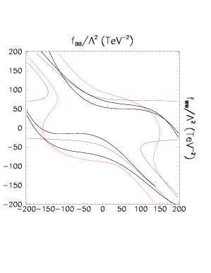
Figure 1: a)Exclusion region outside the curves in the $f_{BB}\times f_{WW}$ plane, in TeV^-2, based on the CDF analysis of $\gamma\gamma\gamma$ production (most external black lines), on the D0 analysis of $\gamma\gamma jj$ production (most internal black lines), on the D0 analysis of $\gamma\gamma\not\!\!E_{T}$ (blue lines), and on the OPAL analysis of $\gamma\gamma\gamma$ production (red lines) , always assuming $M_{H}=100$ GeV. The curves show the 95% CL deviations from the SM total cross section. b) Same as a) for all processes combined.

These bounds depend on the Higgs mass and became weaker as the Higgs boson becomes heavier. In Table 1 we display the allowed values for $f/\Lambda^{2}$, at 95% CL, from $\gamma\gamma jj$ Tevatron D0 data analysis assuming that $f_{WW}=f_{BB}$ and $f_{W}=f_{B}=0$ for different Higgs masses. For the sake of completeness we also show the accessible bound for future Tevatron Upgrades. We should remind that this scenario will not be restricted by data on $W^{+}W^{-}$ production since there is no trilinear vector boson couplings involved. Therefore the limits here presented are the only existing direct bounds on these operators.

Table 1: Allowed range of $f/\Lambda^{2}$ in TeV^-2 at 95% CL, assuming that ($f_{BB}=f_{WW}\gg f_{B},f_{W}$) for the different final states, and for different Higgs boson masses

$M_{H}$ (GeV)		100	150	200	250
$j\,j\,\gamma\,\gamma$	RunI	($-20$ — 49)	($-26$ — 64)	($-96$ —$>100$)	($<-100$ — $>100$)
	RunII	($-8.4$ — 26)	($-11$ — 31)	($-36$ — 81)	($-64$ — $>100$)
	TeV33	($-4.2$ — 6.5)	($-4.5$ — 12)	($-19$ — 40)	($-28$ — 51)

One may wonder how reasonable are these bounds, or how they compare with other existing limits on the coefficients of other dimension-six operator. In order to address this question one can make the assumption that all blind operators affecting the Higgs interactions have a common coupling $f$ $\!{}^{{\bf?}}$, i.e.

$$f_{W}=f_{B}=f_{WW}=f_{BB}=f\;,$$ (10)

In this scenario, $g^{(1)}_{HZ\gamma}=g^{(3)}_{HZZ}=0$, and we can relate the Higgs boson anomalous coupling $f$ with the conventional parametrization of the vertex $WWV$ ($V=Z$, $\gamma$)

$$\Delta\kappa_{\gamma}=\frac{M_{W}^{2}}{\Lambda^{2}}~{}f=c^{2}\Delta g^{Z}_{1}\;\;\;,\Delta\kappa_{Z}=\frac{(1-2s^{2})}{c^{2}}\Delta\kappa_{\gamma}\;\;.$$ (11)

In Fig. 2, we show the region in the $\Delta\kappa_{\gamma}\times M_{H}$ that can be excluded through the combined analysis of the $\gamma\gamma\gamma$ production at LEP, $\gamma\gamma\gamma$, $\gamma\gamma+\!\!E_{T}$, and $\gamma\gamma jj$ production at Tevatron $\!{}^{{\bf?}}$.

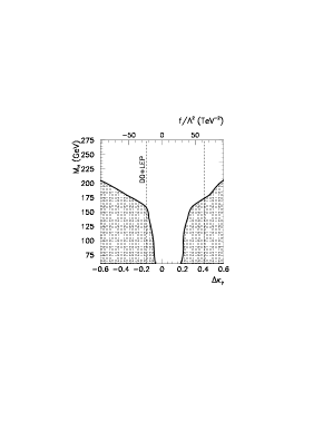
Figure 2: Excluded region in the $\Delta\kappa_{\gamma}\times M_{H}$ plane from the combined analysis from the combined results of the $\gamma\gamma\gamma$ production at LEP, $\gamma\gamma\gamma$, $\gamma\gamma+\!\!E_{T}$, and $\gamma\gamma jj$ production at Tevatron, assuming that all $f_{i}$ are equal (see text for details).

For the sake of comparison, we also show in Fig. 2 the best available experimental limit on $\Delta\kappa_{\gamma}$ from double gauge boson production at Tevatron and LEP II $\!{}^{{\bf?}}$. In all cases the results were obtained assuming the HISZ scenario. We can see that, for $M_{H}\leq 170$ GeV, the limit that can be established at 95% CL from the Higgs production analysis is tighter than the present limit coming from gauge boson production.

In conclusion, we have shown that the analysis of an anomalous Higgs boson production at the Fermilab Tevatron and the CERN LEP II collider may be used to impose strong limits on new effective interactions. Under the assumption that the coefficients of the four “blind” effective operators contributing to Higgs–vector boson couplings are of the same magnitude, the study can give rise to a significant indirect limit on anomalous $WW\gamma$ couplings. Furthermore, this analysis is able to set constraints on those operators contributing to new Higgs interactions for Higgs masses far beyond the kinematical reach of LEP II.

References

References

- [1] Based on the work by F. de Campos, M.C. Gonzalez-Garcia y S.F.Novaes, Phys. Rev. Lett. 79, 5210 (1997); M.C. Gonzalez-Garcia, S.M. Lietti, S.F. Novaes, Phys. Rev. D57, 7045 (1998); O.J.P. Eboli, M.C. Gonzalez-Garcia, S.M. Lietti, S.F. Novaes, hep-ph/9802408, To appear in Physics Letters B; F. de Campos, M.C. Gonzalez-Garcia, S.M. Lietti, S.F. Novaes, R. Rosenfeld hep-ph/9806307, To appear In Physics Letters B.
- [2] K. Hagiwara, H. Hikasa, R. D. Peccei and D. Zeppenfeld, Nucl. Phys. B282, 253 (1987).
- [3] C. J. C. Burguess and H. J. Schnitzer, Nucl. Phys. B228, 464 (1983); C. N. Leung, S. T. Love and S. Rao, Z. Phys. 31, 433 (1986); W. Buchmüller and D. Wyler, Nucl. Phys. B268, 621 (1986).
- [4] A. De Rujula, M. B. Gavela, P. Hernandez and E. Masso, Nucl. Phys. B384, 3 (1992); A. De Rujula, M. B. Gavela, O. Pene and F. J. Vegas, Nucl. Phys. B357, 311 (1991).
- [5] K. Hagiwara, S. Ishihara, R. Szalapski and D. Zeppenfeld, Phys. Lett. B283, 353 (1992); idem, Phys. Rev. D48, 2182 (1993); K. Hagiwara, T. Hatsukano, S. Ishihara and R. Szalapski, Nucl. Phys. B496, 66 (1997).
- [6] For a review see: T. Yasuda, report FERMILAB–Conf–97/206–E, and hep–ex/9706015.
- [7] F. Abe et al., CDF Collaboration, Phys. Rev. Lett. 74, 1936 (1995); idem 74, 1941 (1995); idem 75, 1017 (1995); idem 78, 4536 (1997).
- [8] S. Abachi et al., DØ Collaboration, Phys. Rev. Lett. 75, 1023 (1995); idem 75, 1028 (1995); idem 75, 1034 (1995); idem 77, 3303 (1996); idem 78, 3634 (1997); idem 78, 3640 (1997).
- [9] B. Abbott et al., DØ Collaboration, Phys. Rev. Lett. 79, 1441 (1997).
- [10] For a review see: Z. Ajaltuoni et al., “Triple Gauge Boson Couplings”, in Proceedings of the CERN Workshop on LEP II Physics, edited by G. Altarelli, T. Sjöstrand, and F. Zwirner, CERN 96–01, Vol. 1, p. 525 (1996), and hep-ph/9601233.
- [11] T. Barklow et al., Summary of the Snowmass Subgroup on Anomalous Gauge Boson Couplings, to appear in the Proceedings of the 1996 DPF/DPB Summer Study on New Directions in High-Energy Physics, June 25 — July 12 (1996), Snowmass, CO, USA, and hep-ph/9611454.
- [12] D. Amidei et al., Future Electroweak Physics at the Fermilab Tevatron: Report of the TeV–2000 Study Group, preprint FERMILAB-PUB-96-082 (1996).
- [13] K. Hagiwara, R. Szalapski and D. Zeppenfeld, Phys. Lett. B318, 155 (1993).
- [14] B. Abbott et al., DØ Collaboration, FERMILAB-CONF-97/325-E, contribution to the Lepton-Photon Conference, Hamburg, July 1997.
- [15] A. Stange, W. Marciano, and S. Willenbrock, Phys. Rev. D49, 1354 (1994); Phys. Rev. D50, 4491 (1994).
- [16] J. F. Gunion, H. E. Haber, G. Kane, S. Dawson, The Higgs Hunter’s Guide (Addison–Wesley, 1990).
- [17] V. Barger, T. Han , D. Zeppenfeld, and J. Ohnemus, Phys. Rev. D41, 2782 (1990).
- [18] T. Stelzer and W. F. Long, Comput. Phys. Commun. 81, 357 (1994).
- [19] H. Murayama, I. Watanabe and K. Hagiwara, KEK report 91-11 (unpublished).
- [20] A. D. Martin, W. J. Stirling, R. G. Roberts Phys. Lett. B354, 155 (1995).
- [21] S. Abachi et al., DØ Collaboration, Phys. Rev. Lett. 78, 2070 (1997).
- [22] B. Abbott et al., DØ Collaboration, Phys. Rev. Lett. 80, 442 (1998).
- [23] OPAL Collaboration, K. Ackerstaff et al., Eur. Phys. J. C1 (1998) 31.
- [24] OPAL Collaboration, K. Ackerstaff et al., Eur. Phys. J. C1 (1998) 21.
- [25] F. Abe et al., CDF Collaboration, Phys. Rev. Lett. 81, 1791 (1998).
- [26] M. C. Gonzalez–Garcia, S. M. Lietti, and S. F. Novaes, in preparation.
- [27] See for instace, talks by T. Diehl and H. Phillips in these proceedings.