MADPH-98-1090 SLAC-PUB-7981 November 1998

Top-Charm Associated Production in High Energy $e^{+}e^{-}$ Collisions

Tao Han^(a) and JoAnne L. Hewett^(b)

^(a)Department of Physics, University of Wisconsin, Madison, WI 53706

^(b)Stanford Linear Accelerator Center, Stanford CA 94309, USA

The possibility of exploring the flavor changing neutral current $tcZ/tc\gamma$ couplings in the production vertex for the reaction $e^{+}e^{-}\rightarrow t\bar{c}+\bar{t}c$ is examined. Using a model independent parameterization for the effective Lagrangian to describe the most general three-point interactions, production cross sections are found to be relatively small at LEP II, but potentially sizeable at higher energy $e^{+}e^{-}$ colliders. The kinematic characteristics of the signal are studied and a set of cuts are devised for clean separation of the signal from background. The resulting sensitivity to anomalous flavor changing couplings at LEP II with an integrated luminosity of $4\times 500$ pb^-1 is found to be comparable to their present indirect constraints from loop processes, while at higher energy colliders with $0.5-1$ TeV center-of-mass energy and $50-200$ fb^-1 luminosity, one expects to reach a sensitivity at or below the percentage level.

1 Introduction

It is often stated that the large value of the top-quark mass opens the possibility that it plays a special role in particle physics. Indeed, the properties of the top-quark could reveal information on the nature of electroweak symmetry breaking, address questions in flavor physics, or provide special insight to new interactions originating at a higher scale. One consequence of its large mass is that top decays rapidly via $t\rightarrow W+b$, before the characteristic time for hadron formation and hence top-flavored meson states do not form. This results in a fundamentally different phenomenology for top than for the lighter quark states and allows for the unique capability to determine the properties of the quark itself[1]. The precise determination of these properties may well reveal the existence of physics beyond the Standard Model (SM)[2].

One possible manifestation of new interactions in the top-quark sector is to alter its couplings to the gauge bosons. Such anomalous couplings would modify top production and decay at colliders[3], as well as affecting loop-induced processes[4]. The most widely studied cases are the $t\bar{t}V$, with $V=\gamma\,,Z\,,g$, and $tbW$ three-point functions. However, the flavor changing neutral current (FCNC) interactions $t\bar{c}V\,,t\bar{u}V$ also offer an ideal place to search for new physics as they are very small in the SM[5]. In this instance any positive observation of these transitions would unambiguously signal the presence of new physics. The FCNC vertices can be probed either directly in top-quark decays, indirectly in loops, or via the production vertex for top plus light quark associated production. It is the latter case which is studied here in the reaction

$$e^{+}e^{-}\rightarrow t\bar{c}+\bar{t}c.$$ (1)

As will be discussed below, this mechanism offers some advantages due to the ability to probe higher dimension operators at large momenta and to striking kinematic signatures which are straightforward to detect in the clean environment of $e^{+}e^{-}$ collisions.

2 Top FCNC Interactions

Deviations from the SM for the flavor changing vertices can be described by a linear effective Lagrangian which contains operators in an expansion series in powers of $1/\Lambda$, where $\Lambda$ is a high mass scale characteristic of the new interactions. In this case the lowest dimension gauge invariant operators built from SM fields are dimension six and can be written as[6, 7]

$${\cal L}_{eff} = {\alpha_{B}\over\Lambda^{2}}\bar{Q}_{L}\sigma^{\mu\nu}c_{R}\tilde{\Phi}B_{\mu\nu}+{\alpha_{W}\over\Lambda^{2}}\bar{Q}_{L}\sigma^{\mu\nu}c_{R}\tilde{\Phi}\tau_{a}W^{a}_{\mu\nu}$$ (2)

$$+{\tilde{\alpha}_{B}\over\Lambda^{2}}\bar{Q}_{L}\sigma^{\mu\nu}i\gamma_{5}c_{R}\tilde{\Phi}B_{\mu\nu}+{\tilde{\alpha}_{W}\over\Lambda^{2}}\bar{Q}_{L}\sigma^{\mu\nu}i\gamma_{5}c_{R}\tilde{\Phi}\tau_{a}W^{a}_{\mu\nu}+h.c.\,,$$

with $W^{a}_{\mu\nu}\,,B_{\mu\nu}$ being the field strength tensors for the three non-abelian fields of SU(2)_L and the single abelian gauge field associated with U(1)_Y respectively, $\tilde{\Phi}$ is the conjugate Higgs field $\tilde{\Phi}=i\tau_{2}\Phi^{*}$, $\tau_{a}$ are the Pauli spin matrices, and $Q_{L}$ represents the third generation left-handed quark doublet. This effective Lagrangian is then added to that of the SM and after spontaneous symmetry breaking it induces the dimension five operators in

$${\cal L} = e\bar{t}{i\sigma_{\mu\nu}q^{\nu}\over m_{t}+m_{c}}(\kappa_{\gamma}-i\tilde{\kappa}_{\gamma}\gamma_{5})cA^{\mu}$$

$$+{g\over 2c_{w}}\bar{t}\left[\gamma_{\mu}(v_{Z}-a_{Z}\gamma_{5})+{i\sigma_{\mu\nu}q^{\nu}\over m_{t}+m_{c}}(\kappa_{Z}-i\tilde{\kappa}_{Z}\gamma_{5})\right]cZ^{\mu}+h.c.\,,$$

where $q$ labels the momentum of the gauge boson. The dimension four terms can arise from anomalous contributions of terms like $(v^{2}/\Lambda^{2})\bar{\psi}_{i}\gamma_{\mu}D^{\mu}\psi_{j}$, where $v$ represents the vacuum expectation value of the SM Higgs field and $D^{\mu}$ is the covariant derivative. The coefficients of the dimension five terms are related to those of the dimension six operators above by

$${e\over m_{t}+m_{c}}~{}^{(}\tilde{\kappa}^{)}_{\gamma} = {\sqrt{2}v\over\Lambda^{2}}(c_{w}~{}^{(}\tilde{\alpha}_{B}^{)}+s_{w}~{}^{(}\tilde{\alpha}_{W}^{)})\,,$$

$${g\over 2c_{w}(m_{t}+m_{c})}~{}^{(}\tilde{\kappa}^{)}_{Z} = {\sqrt{2}v\over\Lambda^{2}}(s_{w}~{}^{(}\tilde{\alpha}_{B}^{)}-c_{w}~{}^{(}\tilde{\alpha}_{W}^{)})\,.$$ (4)

In the flavor conserving case, $\kappa$ and $\tilde{\kappa}$ are the magnetic and electric dipole moment form factors, respectively, of the fermion to the $\gamma$ and $Z$. Note that the $\tilde{\kappa}$ terms are CP-violating. It is also possible to derive these operators from a non-linear effective Lagrangian approach[8], where the exact form of Eq. (2) can be derived in the unitary gauge with prescribed relations[7] between the form factors and the parameters of the chiral expansion. In principle, the operator $e\bar{t}F(q^{2})(\gamma_{\mu}q^{2}-q_{\mu}\not q)cA^{\mu}$ can also mediate FCNC interactions for non-zero values of $q^{2}$, i.e., $F(q^{2}=0)=0$, but we do not consider this possibility here. In the following, we employ Eq. (2) as a model independent parameterization of the effects of new physics on the FCNC three-point function and assume that the form factors are static.

It is instructive to roughly estimate the relative sizes of the anomalous couplings. It is sensible to assume that the couplings $\alpha,\tilde{\alpha}$ in Eq. (2) are naturally of ${\cal O}(1)$. We thus expect that $\kappa,\tilde{\kappa}$ as well as $a_{Z},v_{Z}$ in Eq. (2) to be of ${\cal O}(0.1)$. This estimate of course depends on the normalization scale which we have conveniently chosen as $m_{t}$ in order to correspond to the traditional dipole moment form factor definitions. If we took it to be scaled by $\Lambda=1$ TeV instead, then the $\kappa$’s would be roughly of order 1.

A convenient way to compare the sensitivity of various processes to these anomalous form factors, as well as to evaluate their expected values in different models, is to relate them to the FCNC partial widths of the top-quark. In the case of the dimension four operators, this can be readily computed and gives the branching fraction

$${\Gamma_{4}(t\rightarrow cZ)\over\Gamma(t\rightarrow bW)}={(m_{t}^{2}-M_{Z}^{2})^{2}(m_{t}^{2}+2M_{Z}^{2})\over(m_{t}^{2}-M_{W}^{2})^{2}(m_{t}^{2}+2M_{W}^{2})}\ (v_{Z}^{2}+a_{Z}^{2})\simeq(v_{Z}^{2}+a_{Z}^{2})\,.$$ (5)

For the dimension five operators, the results in the on-shell case are

$${\Gamma_{5}(t\rightarrow cZ)\over\Gamma(t\rightarrow bW)}={(m_{t}^{2}-M_{Z}^{2})^{2}(m_{t}^{2}+3/2M_{Z}^{2})\over(m_{t}^{2}-M_{W}^{2})^{2}(m_{t}^{2}+2M_{W}^{2})}\ {2M_{Z}^{2}\over m_{t}^{2}}\ (\kappa_{Z}^{2}+\tilde{\kappa}_{Z}^{2})\simeq\ 0.55(\kappa_{Z}^{2}+\tilde{\kappa}_{Z}^{2})\,.$$ (6)

and

$${\Gamma_{5}(t\rightarrow c\gamma)\over\Gamma(t\rightarrow bW)}={m_{t}^{6}\over(m_{t}^{2}-M_{W}^{2})^{2}(m_{t}^{2}+2M_{W}^{2})}\ {4M_{W}^{2}\over m_{t}^{2}}\sin^{2}\theta_{W}\ (\kappa_{\gamma}^{2}+\tilde{\kappa}_{\gamma}^{2})\simeq\ 0.3(\kappa_{\gamma}^{2}+\tilde{\kappa}_{\gamma}^{2})\,.$$ (7)

As previously mentioned, the top FCNC branching fractions are unmeasureably small in the SM[5] with $B(t\rightarrow c\gamma\,,cZ)=5.2\times 10^{-13}\,,1.5\times 10^{-13}$, respectively, for $m_{t}=175$ GeV. Substantial enhancements of $4-5$ orders of magnitude can be obtained[5, 9] in flavor conserving Two-Higgs-Doublet models and Supersymmetry, however the resulting branching ratios remain small being of order $10^{-9}-10^{-8}$ at the largest. Flavor changing Multi-Higgs-Doublet models bring further enhancements[10] with $B(t\rightarrow cV)\sim 10^{-6}-10^{-5}$ being possible. However, models with singlet quarks[11] which contain tree-level FCNC, compositeness models[12], or models of dynamical electroweak symmetry breaking[13], which can all introduce effective flavor changing couplings of ${\cal O}(\sqrt{m_{t}m_{c}}/v)$, can yield sizeable branching fractions of $B(t\rightarrow cV)\mathrel{\mathchoice{\lower 3.01385pt\vbox{\halign{$\matth\displaystyle\hfil#\hfil$\cr<\crcr\sim\crcr}}}{\lower 3.01385pt\vbox{\halign{$\matth\textstyle\hfil#\hfil$\cr<\crcr\sim\crcr}}}{\lower 3.01385pt\vbox{\halign{$\matth\scriptstyle\hfil#\hfil$\cr<\crcr\sim\crcr}}}{\lower 3.01385pt\vbox{\halign{$\matth\scriptscriptstyle\hfil#\hfil$\cr<\crcr\sim\crcr}}}}1\%$.

Some models which induce FCNC are more naturally probed via top-charm associated production than in flavor changing top-quark decays due to the large underlying mass scales and possibly large momentum transfer. An illustration of this, which is particularly well suited to the reaction considered here, is that of Topcolor assisted Technicolor[14]. Tree-level FCNC for the additional neutral gauge boson present in this model are generated when the quark fields are rotated to the mass eigenstate basis. The couplings of this $Z^{\prime}$ are non-universal and stronger for the third generation, yielding potentially large $tcZ^{\prime}$ interactions. In addition, the production rate for this $Z^{\prime}$, which is constrained[15] to be heavier than $\sim 1.5$ TeV, is sizeable in high energy $e^{+}e^{-}$ collisions[16], and hence $e^{+}e^{-}\rightarrow t\bar{c}+\bar{t}c$ is the ideal place to search for this effect. Another example is given by Multi-Higgs-Doublet models with tree-level FCNC. In this case, s-channel Higgs exchange can mediate top-charm production at interesting levels at muon[17] and $\gamma\gamma$[18] colliders.

Present constraints on the anomalous couplings in Eq. (2) arise from a variety of processes. A global analysis of the flavor changing neutral current processes $K_{L}\rightarrow\mu^{+}\mu^{-}\,,B\rightarrow\ell^{+}\ell^{-}X\,,K_{L}-K_{S}$ mass difference, and $B^{0}-\bar{B}^{0}$ mixing, as well as the oblique parameters in electroweak precision measurements has been performed[19] for the dimension four operators by forming a low-energy effective interaction after integrating out the heavy top-quark. This procedure yields the restrictions

$$g_{L}^{Z}=v_{Z}-a_{Z} \leq 0.05\,,$$

$$g_{R}^{Z}=v_{Z}+a_{Z} \leq 0.29\,,$$ (8)

assuming a cutoff of 1 TeV. Bounds on the $tc\gamma$ interactions can be obtained from $B\rightarrow X_{s}\gamma$ and restrict[20] $|\kappa_{\gamma}|<0.1$, using the normalization in (2) and assuming $\tilde{\kappa}_{\gamma}=0$. CDF has performed a direct search for FCNC top decays and has placed[21] the $95\%$ C.L. limits of $B(t\rightarrow q\gamma)<3.2\%$ and $B(t\rightarrow qZ)<33\%$, where $q=c$ or $u$. In the photonic channel, this gives the constraint of $\kappa_{\gamma}\mathrel{\mathchoice{\lower 3.01385pt\vbox{\halign{$\matth\displaystyle\hfil#\hfil$\cr<\crcr\sim\crcr}}}{\lower 3.01385pt\vbox{\halign{$\matth\textstyle\hfil#\hfil$\cr<\crcr\sim\crcr}}}{\lower 3.01385pt\vbox{\halign{$\matth\scriptstyle\hfil#\hfil$\cr<\crcr\sim\crcr}}}{\lower 3.01385pt\vbox{\halign{$\matth\scriptscriptstyle\hfil#\hfil$\cr<\crcr\sim\crcr}}}}0.26$, which is not yet competitive with the indirect bounds from $B\rightarrow X_{s}\gamma$. The $Z$ decay channel is not yet at an interesting level of sensitivity. These direct constraints from top decays are expected[19, 20] to improve to the level of $\kappa_{\gamma}\simeq 0.04$ and $\sqrt{v_{Z}^{2}+a_{Z}^{2}}\simeq 0.11$ during Run II at the Tevatron with $10~{}{\rm fb}^{-1}$ of integrated luminosity, and $\kappa_{\gamma}\simeq 0.0035$ and $\sqrt{v_{Z}^{2}+a_{Z}^{2}}\simeq 0.014$ at the LHC with $100~{}{\rm fb}^{-1}$ of integrated luminosity. In addition, a $\sqrt{s}=400$ GeV photon collider can probe[22] $\kappa_{\gamma}$ down to values of $\simeq 0.01$ with $10~{}{\rm fb}^{-1}$ of integrated luminosity via the reaction $\gamma\gamma\rightarrow t\bar{q}+\bar{t}q$. Similar studies have also been performed[23] for analogous anomalous $tcg$ couplings.

The production rate for $e^{+}e^{-}\rightarrow t\bar{c}+\bar{t}c$ was first computed in Ref. [24] with the dimention-four terms. They have been later studied for the case with leptoquark exchanges [25], and for the case of flavor non-conserving Multi-Higgs-Doublet models in Ref. [26], in Supersymmetry with R-parity violation [27], and for some models of mass matrix textures[28]. The SM one-loop induced production in $e^{+}e^{-}$ collisions was discussed in [29] and other higher order processes, such as $e^{+}e^{-}\rightarrow t\bar{c}\nu_{e}\bar{\nu}_{e}$, have also been considered[30]. It is the intention of this work to study the model independent case, and to, more importantly, investigate the issue of detecting the signal over the background and to determine to what precision the FCNC couplings in Eq. (2) can be measured in $e^{+}e^{-}$ collisions. We note that the analysis presented here can also be applied to top-up-quark associated production.

3 Top-Charm Associated Production

3.1 The Total Cross Section

We now investigate top-charm associated production in high energy $e^{+}e^{-}$ collisions. This process is mediated by $s$-channel $\gamma^{*},Z$ exchange,

$$e^{+}e^{-}\rightarrow\gamma^{*},Z\rightarrow t\bar{c}+\bar{t}c\,,$$ (9)

via the FCNC couplings. Using the effective Lagrangian in Eq. (2) the differential cross section is calculated to be

$${d\sigma\over dz} = {3\pi\alpha^{2}\over 2s}\left(1-{m_{t}^{2}\over s}\right)^{2}\sum_{i,j=\gamma,Z}P_{ij}\left\{B_{ij}\left[\left(1+{m_{t}^{2}\over s}\right)+\left(1-{m_{t}^{2}\over s}\right)z^{2}\right]\right.$$ (10)

$$\left.+2C_{ij}z+{s\over m_{t}^{2}}D_{ij}\left[\left(1+{m_{t}^{2}\over s}\right)-\left(1-{m_{t}^{2}\over s}\right)z^{2}\right]+2E_{ij}+2F_{ij}z\right\}\,,$$

where $z=\cos\theta$ with $\theta$ being the angle between the top-quark and the electron. The usual propagator factor is defined as

$$P_{ij}={s^{2}[(s-M_{i}^{2})(s-M_{j}^{2})+(\Gamma_{i}M_{i})(\Gamma_{j}M_{j})]\over[(s-M_{i}^{2})^{2}+(\Gamma_{i}M_{i})^{2}][(s-M_{j}^{2})^{2}+(\Gamma_{j}M_{j})^{2}]}\,,$$ (11)

where $M_{i}\,,\Gamma_{i}$ refer the mass and width of the $ith$ gauge boson, and the coupling factors are

$$B_{ij} = (v_{i}v_{j}+a_{i}a_{j})_{e}(v_{i}v_{j}+a_{i}a_{j})_{tc}\,,$$

$$C_{ij} = (v_{i}a_{j}+v_{j}a_{i})_{e}(v_{i}a_{j}+v_{j}a_{i})_{tc}\,,$$

$$D_{ij} = (v_{i}v_{j}+a_{i}a_{j})_{e}(\kappa_{i}\kappa_{j}+\tilde{\kappa}_{i}\tilde{\kappa}_{j})_{tc}\,,$$ (12)

$$E_{ij} = (v_{i}v_{j}+a_{i}a_{j})_{e}(v_{i}\kappa_{j}+v_{j}\kappa_{i})_{tc}\,,$$

$$F_{ij} = (v_{i}a_{j}+v_{j}a_{i})_{e}(a_{i}\kappa_{j}+a_{j}\kappa_{i})_{tc}\,,$$

with $v_{\gamma}=a_{\gamma}=0$. The terms proportional to $C_{ij},F_{ij}$ are odd in $z$ and will produce an asymmetric angular distribution if more than one anomalous coupling is simultaneously non-vanishing. Due to the $\sigma_{\mu\nu}q^{\nu}$ structure of the dimension five operator, the term proportional to $D_{ij}$ does not have the usual $1/s$ dependence and will dominate the cross section as the center-of-mass energy increases. Note that if only one anomalous coupling is non-zero at a time (as we will assume implicitly unless stated otherwise), then the integrated cross section is directly proportional to its square. Figure 1 displays the total cross section as a function of the center-of-mass energy, taking only one coupling non-vanishing at a time with either $\kappa_{\gamma}=1(0.1)$, $\kappa_{Z}=1(0.1)$, or $v_{Z}=1(0.1)$. These values were chosen for purposes of demonstration only, and the property that the cross section is proportional to the square of the coupling is explicitly demonstrated. From Eq. (10) it is clear that taking $v_{Z}$ versus $a_{Z}$ (or $\tilde{\kappa}_{\gamma,Z}$ versus $\kappa_{\gamma,Z}$) to be non-zero yields the same numerical result.

Figure 1: Cross section for top-charm associated production as a function of center-of-mass energy in $e^{+}e^{-}$ collisions. Only one anomalous coupling is taken to be non-zero at a time, with values as indicated.

3.2 Signal And Background

We concentrate on the semi-leptonic decay of the single top-quark,

$$e^{+}e^{-}\rightarrow\bar{c}t\rightarrow\bar{c}b\ \ell\nu_{\ell},$$ (13)

to efficiently separate the signal from the SM background, taking $\ell=e$ or $\mu$, and the charge-conjugate state is implied. The irreducible SM background arises from $e^{+}e^{-}\rightarrow W^{+}W^{-}\rightarrow\bar{c}b\ell\nu$ and is fortunately negligible due to the small size of the Cabbibo-Kobayashi-Maskawa mixing matrix element $V_{cb}$. However, without the ability to perfectly tag heavy flavor states, light quark jets are also a source of background. The leading SM background then comes from the final state

$$e^{+}e^{-}\rightarrow\bar{q}q^{\prime}\ell\nu,$$ (14)

where $q,q^{\prime}$ are light quarks. This originates mainly from $W$ pair production as well as from $W$ bremsstrahlung in $e^{+}e^{-}\rightarrow W+$2-jets. The total cross sections, including the leptonic branching fractions and with no kinematical cuts, are presented in Table 1 for the signal Eq. (13) and the background Eq. (14) for three representative center-of-mass energies at $e^{+}e^{-}$ colliders. The signal cross sections are evaluated with one anomalous coupling to be non-zero (equal to unity) at a time. The results for $\kappa_{\gamma},v_{Z}$ and $\kappa_{Z}$ are the same as those for $\tilde{\kappa}_{\gamma},a_{Z}$ and $\tilde{\kappa}_{Z}$, respectively. We see that for these large values of $\kappa_{\gamma,Z}$ the cross sections for the dimension five operators are already competitive with the background rates, even before any kinematical cuts are applied.

	192 GeV	0.5 TeV	1 TeV
signal[$\kappa_{\gamma}=1$]	156	1980	2070
signal[$v_{Z}=1$]	114	217	60
signal[$\kappa_{Z}=1$]	130	1060	1050
bckgrnd	5687	2252	864

Table 1: Total cross sections in fb for signal Eq. (13) and background Eq. (14) including the leptonic branching fractions and with no kinematical cuts.

To roughly simulate the experimental environment, we first adopt the basic kinematical cuts on the energy and pseudo-rapidity for the jets and leptons

$$E_{j,\ell}>10\ {\rm GeV},\quad|\eta_{j,\ell}|<2,$$ (15)

which corresponds to a 15-degree polar angle with respect to the beam. We also smear the energies with a Gaussian standard deviation of the detector response[31]

$$\Delta E/E=40\%,\quad 10\%,$$ (16)

for jets and leptons, respectively.

Although the signal cross section is not expected to be very large for values of the anomalous couplings which are consistent with model expectations, the signal final state can be quite characteristic in comparison with the background events. First, due to the nature of two-body kinematics for the signal, the charm-jet energy is fixed as

$$E_{c}={\sqrt{s}\over 2}(1-m_{t}^{2}/s),$$ (17)

which leads to the values of $E_{c}\simeq 16\,,220$, and 485 GeV at $\sqrt{s}=192\,,500$, and 1000 GeV, respectively. Similarly, the $b$-quark energy from the top-quark decay in the signal is typically $E_{b}={m_{t}/2}(1-M_{W}^{2}/m_{t})\approx 70$ GeV, modulo some smearing from the top-quark motion. In addition, the signal jets are more central than those arising from the background sources in which there is a strong boost of the $W$ system at higher energies. These features are displayed in Fig. 2 for $\sqrt{s}=500$ GeV. From Fig. 2(a), we see that in contrast to the nearly mono-value for the energy of the harder jet in the case of the signal, the corresponding distribution for the background is uniformly distributed. Fig. 2(b) shows the difference in the rapidity distribution between the signal and the background. Secondly, the charged lepton momentum for the SM background tends to be parallel to that of the parent $W^{\pm}$ boson, while the opposite holds for the signal. This is due to spin correlation effects for transversely polarized $W$ bosons. Consequently, the charged lepton energy distribution for the background is harder due to the parallel boost by the $W$ system, while it is softer for the signal. This is shown in Fig. 3, where (a) the $E_{\ell}$ spectra for the signal and the background are contrasted, and (b) the rapidity distributions are presented. Another apparent difference between the signal and background kinematical features is that the di-jet invariant mass for the background events primarily reconstructs to $M_{W}$, as depicted in Fig. 4(a). Finally, the most important confirmation of the signal is the reconstruction of the top-quark mass. Although the missing energy from the final state neutrino prevents a direct mass measurement of the top-quark, $m_{t}$ can still be accurately reconstructed from knowledge of the center-of-mass energy and the charm jet energy via

$$m_{t}^{\rm rec}=(s-2{\sqrt{s}}E_{c})^{1/2}.$$ (18)

This variable is depicted in Fig. 4(b) for $\sqrt{s}=500$ GeV, where the discrimination power against the SM background is clearly observable. The width of the $m_{t}^{\rm rec}$ distribution increases at higher energies due to the larger charm-jet energy smearing.

Figure 2: Normalized jet-energy and rapidity distributions at $\sqrt{s}=500$ GeV. (a) Jet energy distributions for the signal (S) and background (B) with the harder jet being labeled as $E_{j}^{max}$ and the softer jet as $E_{j}^{min}$. (b) Jet rapidity distribution for the signal and the background.

Figure 3: (a) Normalized lepton-energy and (b) rapidity distributions at $\sqrt{s}=500$ GeV for the signal (solid) and background (dashes).

Figure 4: Normalized distributions for the signal (solid) and background (dashes) at $\sqrt{s}=500$ GeV; (a) di-jet invariant mass distributions, and (b) the reconstructed top-quark mass according to Eq. (18).

The above kinematical results presented in Figs. 2-4 provide the motivation for the optimization of our selective cuts. These cuts are delineated in Table 2. Employing these cuts, the cross sections are then calculated under the reconstructed top-quark mass peak (as prescribed in the last column in Table 2) with the results being given in Table 3. Here we see that our choice of kinematical cuts are very efficient in reducing the size of the background while retaining the signal.

$\sqrt{s}$	$E_{j}$(high)	$E_{j}$(low)	$|M_{jj}-M_{W}|$	$E_{\ell}$	$|m_{t}^{\rm rec}-m_{t}|$
192 GeV	$>60$ GeV	$<20$ GeV	$>10$ GeV	-	$<5$ GeV
500 GeV	$>200$ GeV	$>20$ GeV	$>10$ GeV	$<150$ GeV	$<40$ GeV
1 TeV	$>460$ GeV	$>20$ GeV	$>10$ GeV	$<350$ GeV	$<100$ GeV

Table 2: Kinematical cuts for the event selection at different collider energies.

	192 GeV	0.5 TeV	1 TeV
signal[$\kappa_{\gamma}=1$]	129	1690	1880
signal[$v_{Z}=1$]	95	169	49.7
signal[$\kappa_{Z}=1$]	108	900	951
bckgrnd	23.6	5.1	1.7

Table 3: Total cross sections in fb for the signal Eq. (13) and background Eq. (14) including the leptonic branching fractions and with the kinematical cuts presented in Table 2.

3.3 Sensitivity to the anomalous couplings

Given the efficient signal identification and substantial background suppression achieved in the previous section, we now estimate the sensitivity to the anomalous couplings from this reaction using Gaussian statistics, which is applicable for large event samples. Here,

$$\sigma={N_{S}\over\sqrt{N_{S}+B_{S}}},$$ (19)

with $N_{S}$ and $N_{B}$ being the number of signal and background events. We demand that $\sigma\geq 3$ in order to observe the signal, which approximately corresponds to the $95\%$ Confidence Level.

At LEPII energies, the results in Table 3 demonstrate that the $W^{+}W^{-}$ background is large while the signal rate is relatively low. Figure 5 presents the $95\%$ C.L. sensitivity to the FCNC couplings as a function of the integrated luminosity, summed over all four detectors, with $\sqrt{s}=192$ GeV for $\kappa_{\gamma}(\tilde{\kappa}_{\gamma})$, $v_{Z}(a_{Z})$, and $\kappa_{Z}(\tilde{\kappa}_{Z})$. We see that the combined sensitivity for 500 pb^-1 per detector could reach the 0.3$-$0.4 level. This is similar to (or slightly worse than) the current indirect constraints obtained from rare decays. Since the $b$-flavor tagging efficiency is not very high at LEPII, being only $\sim 25-30\%$, requiring a tagged $b$ in the final state actually decreases the achievable sensitivity.

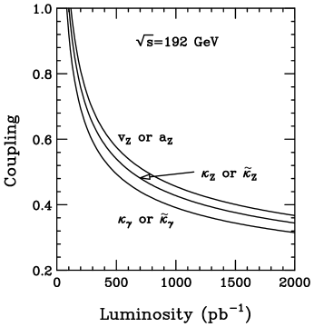
Figure 5: $95\%$ C.L. sensitivity to the FCNC couplings at LEPII with $\sqrt{s}=192$ GeV as a function of integrated luminosity, summed over all four detectors.

At higher energies, the ability to probe the existence of FCNC anomalous couplings is greatly improved. Figures 6 and 7 display the $95\%$ C.L. sensitivity to the couplings as a function of integrated luminosity at $\sqrt{s}=0.5$ and 1 TeV for $\kappa_{\gamma}(\tilde{\kappa}_{\gamma})$, $v_{Z}(a_{Z})$, and $\kappa_{Z}(\tilde{\kappa}_{Z})$. Here, the solid curves correspond to the results using the kinematical cuts only, while the dashed curves include the effects of b-tagging. It is expected[32] that a CCD-based pixel vertex detector combined with topological vertexing can achieve a $\sim 60\%$ b-quark identification efficiency with very high purity at high energy linear colliders. This is not too far of an extrapolation from the present $\sim 50\%$ b-quark identification efficiency that has recently been attained at SLD[33]. We have extended the integrated luminosity for the 0.5 TeV linear collider to 500 fb^-1, corresponding to expectations from the TESLA linear collider design[34]. The sensitivity to these couplings scales with the integrated luminosity ($L$) approximately as $1/\sqrt{L}$ when the background is small. As a result, the ability to explore the FCNC couplings is improved by more than a factor of 2 when the integrated luminosity is increased from 50 to 500 fb^-1. We also note that the sensitivity to the couplings of the dimension five operators, $~{}^{(}\tilde{\kappa}^{)}_{\gamma},~{}^{(}\tilde{\kappa}^{)}_{Z}$, is increased by roughly $30\%$ as the center-of-mass energy is raised from 0.5 to 1 TeV. This is as expected due to the structure of these operators.

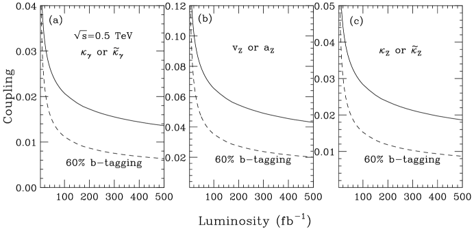
Figure 6: $95\%$ C.L. sensitivity to the FCNC couplings as a function of the integrated luminosity with $\sqrt{s}=500$ GeV for (a) $\kappa_{\gamma}$, (b) $v_{Z}$, and (c) $\kappa_{Z}$, with and without b-tagging as labeled.

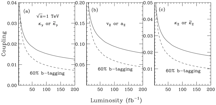
Figure 7: $95\%$ C.L. sensitivity to the FCNC couplings as a function of the integrated luminosity with $\sqrt{s}=1$ TeV for (a) $\kappa_{\gamma}$, (b) $v_{Z}$, and (c) $\kappa_{Z}$, with and without b-tagging as labeled.

4 Asymmetries

As mentioned above, the odd terms in $\cos\theta$ in the cross section generate an asymmetric angular distribution. This is illustrated in Fig. 8 with $\sqrt{s}=500$ GeV for the sample cases of $v_{Z}=a_{Z}=\kappa_{Z}=0.1$ (dashed curve), $a_{Z}=0\,,v_{Z}=\kappa_{Z}=0.1$ (solid), $v_{Z}=0\,,a_{Z}=\kappa_{Z}=0.1$ (dotted), and $v_{Z}=a_{Z}=0.1\,,\kappa_{Z}=0$ (dash-dotted). Note that the case where $a_{Z}=0$ produces a symmetric distribution as expected from the form of the cross section. The other coupling combinations where $a_{Z}$ is non-vanishing all produce distinct asymmetric distributions which can be used to distinguish between the various scenarios. The resulting forward-backward asymmetry and polarized left-right forward-backward asymmetry are displayed in Fig. 9(a) and (b) as a function of the value of the anomalous couplings for $\sqrt{s}=0.5$ and 1 TeV. The coupling combinations taken to be non-zero with equal values are as indicated. The polarized asymmetry is proportional to the FCNC coupling factors

$$A_{FB}^{LR}\sim(v_{i}v_{j}+a_{i}a_{j})_{e}(v_{i}a_{j}+v_{j}a_{i})_{tc}+(v_{i}v_{j}+a_{i}a_{j})_{e}(\kappa_{i}a_{j}+\kappa_{j}a_{i})_{tc}\,.$$ (20)

In Fig. 9 we have taken the degree of beam polarization to be $90\%$ and employ a $10^{\circ}$ angular cut around the beam pipe to remove backgrounds from the interaction region. We see that these two asymmetries have similar shapes, and hence the beam polarization does not add much new information, however, they clearly distinguish between the various options for the non-vanishing couplings. Hence, if top-charm associated production is observed, these asymmetries would provide a valuable tool for discerning the structure of the FCNC couplings and unraveling the underlying physics.

Figure 8: Angular distributions for the cases of $v_{Z}=a_{Z}=\kappa_{Z}=0.1$ (dashed curve), $a_{Z}=0\,,v_{Z}=\kappa_{Z}=0.1$ (solid), $v_{Z}=0\,,a_{Z}=\kappa_{Z}=0.1$ (dotted), and $v_{Z}=a_{Z}=0.1\,,\kappa_{Z}=0$ (dash-dotted) with $\sqrt{s}=500$ GeV.

Figure 9: (a) Forward-backward asymmetry and (b) Left-Right forward-backward asymmetry as a function of the value of the FCNC coupling. The coupling combinations taken to be non-vanishing and equal are as indicated. For the $v_{Z}=a_{Z}$ and $v_{Z}=a_{Z}=\kappa_{Z}$ cases, the solid (dashed) curve corresponds to $\sqrt{s}=0.5$ (1) TeV; the $a_{Z}=\kappa_{Z}$ case is dotted (dash-dotted) for $\sqrt{s}=0.5$ (1) TeV.

5 Conclusions

We have examined the possibility of top-charm associated production in $e^{+}e^{-}$ collisions via FCNC couplings. This mechanism, in contrast to the study of rare top-quark decays, allows for the exploration of higher dimensional operators at large values of momenta. We used a model independent parameterization to describe these couplings and devised a set of cuts to cleanly distinguish the signal from the background. Our results show that LEPII will be able to probe these couplings only at a level which is comparable to the constraints from present data. However, a 500 GeV linear collider with 50 ${\rm fb}^{-1}$ has more sensitivity to these couplings than the Tevatron with 30 fb^-1, and with 500 fb^-1 it is comparable in reach to that of the LHC with 100 fb^-1. The 1 TeV machine gives roughly a $30\%$ improvement in sensitivity. These cases correspond to exploring FCNC top decays with branching ratios in the range $10^{-4}-10^{-3}$. In addition, if $a_{Z}\neq 0$, then angular and polarization asymmetries can be formed which can yield information on the structure of the couplings and the underlying physics.

Acknowledgments: We would like to thank G. Burdman, J. Jaros, F. Paige, M. Peskin, K. Riles and T. Rizzo for discussions related to this work. T.H. was supported in part by a DOE grant No. DE-FG02-95ER40896 and in part by the Wisconsin Alumni Research Foundation.

References

- [1] For recent reviews on top-quark physics, see e.g., R. Frey et al., hep-ph/9704243; S. Willenbrock, hep-ph/9709355; C. Quigg, hep-ph/9802320.
- [2] For recent reviews on top-quark physics beyond the SM, see e.g., E. Simmons, in Physics Beyond the Standard Model V, Balholm, Norway, 29 Apr - 4 May (1997), and references therein; F. Larios, E. Malkawi, and C-.P. Yuan, hep-ph/9704288.
- [3] D. Atwood, A. Aeppli, and A. Soni, Phys. Rev. Lett. 69, 2754 (1992); D. Atwood, A. Kagan, and T.G. Rizzo, Phys. Rev. D52, 6264 (1995); C.R. Schmidt, Phys. Rev. D54, 3250 (1996); K. Cheung, Phys. Rev. D53, 3604 (1996); P. Haberl, O. Nachtmann, and A. Wilch, Phys. Rev. D53, 4875 (1996); T.G. Rizzo, Phys. Rev. D53, 6218 (1996); D. Silverman, Phys. Rev. D54, 5562 (1996); K. Hikasa et al., hep-ph/9806401.
- [4] J.L. Hewett and T.G. Rizzo, Phys. Rev. D49, 319 (1994); R.S. Chivukula, E.H. Simmons, and J. Terning, Phys. Lett. B331, 383 (1994); C.T. Hill and X. Zhang, Phys. Rev. D51, 3563 (1995); E. Nardi, Phys. Lett. B365, 327 (1996).
- [5] G. Eilam, J.L. Hewett, and A. Soni, Phys. Rev. D44, 1473 (1991).
- [6] C. Burgess and H.J. Schnitzer, Nucl. Phys. B228, 464 (1983); W. Buchmüller and D. Wyler, Nucl. Phys. B268, 621 (1986); C.N. Leung, S.T. Love, and S. Rao, Z. Phys. C31, 433 (1986); R. Escribano and E. Masso, Phys. Lett. B301, 419 (1983).
- [7] R. Escribano and E. Masso, Nucl. Phys. B429, 19 (1994).
- [8] T. Appelquist and C. Bernard, Phys. Rev. D22, 200 (1980); A.C. Longhitano, Phys. Rev. D22, 1166 (1980); Nucl. Phys. B191, 146 (1981); R.D. Peccei and X. Zhang, Nucl. Phys. B337, 269 (1990); R.D. Peccei, S. Peris, and X. Zhang, Nucl. Phys. B349, 305 (1991); F. Feruglio, Int. J. Mod. Phys. A8, 4937 (1993); D.O. Carlson, E. Malkawi, and C.-P. Yuan, Phys. Lett. B337, 145 (1994).
- [9] C.S. Li, R.J. Oakes, and J.M. Yang, Phys. Rev. D49, 293 (1994); G. Couture, Hamzaoui, and H. Koenig, Phys. Rev. D52, 1713 (1995); J.L. Lopez, D.V. Nanopoulos, and R. Rangarajan, Phys. Rev. D56, 3100 (1997).
- [10] T.P. Cheng and M. Sher, Phys. Rev. D35, 3484 (1987); B. Mukhopadhyaya and S. Nandi, Phys. Rev. Lett. 66, 285 (1991); W.-S. Hou, Phys. Lett. B296, 179 (1992); L. Hall and S. Weinberg, Phys. Rev. D48, R979 (1993); M. Luke and M. Savage, Phys. Lett. B307, 387 (1993); D. Atwood, L. Reina, A. Soni, Phys. Rev. D55, 3156 (1997).
- [11] V. Barger, M. Berger, and R.J.N. Phillips, Phys. Rev. D52, 1663 (1995).
- [12] H. Georgi, L. Kaplan, D. Morin, and A. Schenk, Phys. Rev. D51, 3888 (1995); R.D. Peccei, in Proceedings of the 1987 Lake Louise Winter Institute:Selected Topics in Electroweak Interactions, ed. J.M. Cameron et al. (World Scientific, Singapore, 1987).
- [13] C.T. Hill, Phys. Lett. B266, 419 (1991); ibid., B345, 483 (1995); B. Holdom, Phys. Lett. B339, 114 (1994); ibid., B351, 279 (1995) ; X. Zhang, Phys. Rev. D51, 5039 (1995); J. Berger, A. Blotz, H.-C. Kim, and K. Goeke, Phys. Rev. D54, 3598 (1996); B.A. Arbuzov and M.Y. Osipov, hep-ph/9802392.
- [14] G. Buchalla, G. Burdman, C.T. Hill, and D. Kominis, Phys. Rev. D53, 5185 (1996); G. Burdman, Phys. Rev. D52, 6400 (1995).
- [15] R.S. Chivukula and J. Terning, Phys. Lett. B385, 209 (1996).
- [16] T.G. Rizzo, in Proceedings of the 1996 DPF/DPB Summer Study on New Directions for High Energy Physics, Snowmass, CO, July 1996, ed. D.G. Cassell et al., (SLAC, Stanford, CA 1997) p. 864.
- [17] D. Atwood, L. Reina, and A. Soni, Phys. Rev. Lett. 75, 3800 (1995).
- [18] W.-S. Hou, and G.-L. Lin, Phys. Lett. B379, 261 (1996); J. Yi et al., Phys. Rev. D57, 4343 (1998).
- [19] T. Han, R.D. Peccei, and X. Zhang, Nucl. Phys. B454, 527 (1995).
- [20] T. Han et al., Phys. Rev. D55, 7241 (1997).
- [21] F. Abe et al., (CDF Collaboration), Phys. Rev. Lett. 80, 2525 (1998).
- [22] K.J. Abraham, K. Whisnant, and B.-L. Young, Phys. Lett. B419, 381 (1998).
- [23] E. Malkawi and T. Tait, Phys. Rev. D54, 5758 (1996); T. Tait and C.-P. Yuan, Phys. Rev. D55, 7300 (1997); M. Hosch, K. Whisnant, and B.-L. Young, Phys. Rev. D56, 5725 (1997); T. Han et al., Phys. Lett. B385, 311 (1996); Phys. Rev. D58, 073008 (1998).
- [24] K. Hikasa, Phys. Lett. B149, 221 (1984).
- [25] V. Barger and K. Hagiwara, Phys. Rev. D37, 3320 (1988).
- [26] D. Atwood, L. Reina, and A. Soni, Phys. Rev. D53, 1199 (1996); and hep-ph/9612388.
- [27] U. Mahanta and A. Ghosal, Phys. Rev. D57, 1735 (1998).
- [28] Y. Koide, hep-ph/9701261.
- [29] C.-H. Chang, X.-Q. Li, J.-X. Wang and Mao-Zhi Yang, Phys. Lett. B313, 389 (1993).
- [30] S. Bar-Shalom, G. Eilam, A. Soni. and J. Wudka, Phys. Rev. Lett. 79, 1217 (1997); Phys. Rev. D57, 2957 (1998); D. Atwood and M. Sher, Phys. Lett. B411, 306 (1997); W.-S. Hou, G.-L. Lin, and C.-Y. Ma, Phys. Rev. D56, 7434 (1997).
- [31] C.J.S. Damerell et al., in Proceedings of the 1996 DPF/DPB Summer Study on New Directions for High Energy Physics, Snowmass, CO, July 1996, ed. D.G. Cassell et al., (SLAC, Stanford, CA 1997) p. 431.
- [32] C.J.S. Damerell and D.J. Jackson, in Proceedings of the 1996 DPF/DPB Summer Study on New Directions for High Energy Physics, Snowmass, CO, July 1996, ed. D.G. Cassell et al., (SLAC, Stanford, CA 1997) p. 442.
- [33] See, for example, S. Fahey (SLD Collaboration), talk presented at XXIXth International Conference on High Energy Physics, ICHEP98, Vancouver, Canada, July 1998.
- [34] See, for example, B. Wiik, talk presented at DESY Theory Workshop, Hamburg, Germany, September 1998.