Abstract

In a general two-Higgs-doublet model (2HDM), without the ad hoc discrete symmetries to prevent tree-level flavor-changing-neutral currents, an extra phase angle in the charged-Higgs-fermion coupling is allowed. We show that the charged-Higgs amplitude interferes destructively or constructively with the standard model amplitude depending crucially on this phase angle. The popular model I and II are special cases of our analysis. As a result of this phase angle the severe constraint on the charged-Higgs boson mass imposed by the inclusive rate of $b\to s\gamma$ from CLEO can be relaxed. We also examine the effects of this phase angle on the neutron electric dipole moment. Furthermore, we also discuss other constraints on the charged-Higgs-fermion couplings coming from measurements of $B^{0}-\overline{B^{0}}$ mixing, $\rho_{0}$, and $R_{b}$.

I. Introduction

One of the most popular extensions of the standard model (SM) is the two-Higgs-doublet model (2HDM) [1], which has two complex Higgs doublets instead of only one in the SM. The 2HDM allows flavor-changing neutral currents (FCNC), which can be avoided by imposing an ad hoc discrete symmetry [2]. One possibility to avoid the FCNC is to couple the fermions only to one of the two Higgs doublet, which is often known as model I. Another possibility is to couple the first Higgs doublet to the down-type quarks while the second Higgs doublet to the up-type quarks, which is known as model II. This model II has been very popular because it is the building block of the minimal supersymmetric standard model. The physical content of the Higgs sector includes a pair of CP-even neutral Higgs bosons $H^{0}$ and $h^{0}$ , a CP-odd neutral boson $A$, and a pair of charged-Higgs bosons $H^{\pm}$.

Models I and II have been extensively studied in literature and tested experimentally. One of the most stringent tests is the radiative decay of $B$ mesons, specifically, the inclusive decay rate of $b\to s\gamma$, which has the least hadronic uncertainties. The SM rate of $b\to s\gamma$ including the improved leading-order logarithmic QCD corrections is predicted [3] to be $(2.8\pm 0.8)\times 10^{-4}$, of which the uncertainty mainly comes from the factorization scale and from the next-to-leading order corrections. In the 2HDM, the rate of $b\to s\gamma$ can be enhanced substantially for large regions in the parameter space of the mass $M_{H^{\pm}}$ of the charged-Higgs boson and $\tan\beta=v_{2}/v_{1}$, where $v_{1}$ and $v_{2}$ are the vacuum expectation values of the two Higgs doublets. CLEO published a result of $b\to s\gamma$ inclusive rate of $(2.32\pm 0.57\pm 0.35)\times 10^{-4}$ in 1995 [5], which is recently updated to $(3.15\pm 0.35\,({\rm stat})\,\pm 0.32\,({\rm sys})\,\pm 0.26\,({\rm mod}))\times 10^{-4}$ in 1998 [6]. ALEPH also published a result of $(3.11\pm 0.80\,({\rm stat})\,\pm 0.72\,({\rm sys})\,)\times 10^{-4}$ [7]. The 95%CL limit published by CLEO is also updated to $2\times 10^{-4}<B(b\to s\gamma)<4.5\times 10^{-4}$ [6]. The data is now more consistent with the SM prediction than before. Hence, the experimental result puts a rather stringent constraint on the charged-Higgs boson mass $M_{H^{\pm}}$ and $\tan\beta$. In model II, the constraint is $M_{H^{\pm}}\mathrel{\raisebox{-2.58334pt}{$\stackrel{{\scriptstyle\textstyle>}}{{\sim}}$}}350$ GeV for $\tan\beta$ larger than 1, and even stronger for smaller $\tan\beta$ [8].

Recently, there have been some studies [9, 10] on a more general 2HDM without the discrete symmetries as in models I and II. It is often referred as model III. FCNC’s in general exist in model III. However, the FCNC’s involving the first two generations are highly suppressed from low-energy experiments, and those involving the third generation is not as severely suppressed as the first two generations. It implies that model III should be parameterized in a way to suppress the tree-level FCNC couplings of the first two generations while the tree-level FCNC couplings involving the third generation can be made nonzero as long as they do not violate any existing experimental data, e.g., $B^{0}-\overline{B^{0}}$ mixing.

In this work, we simply assume all tree-level FCNC couplings to be negligible. Even though in such a simple model the couplings involving Higgs bosons and fermions can have complex phases $e^{i\theta}$. The effects of such extra phases in $b\rightarrow s\gamma$ have been noticed in Ref.[11]. In this paper, we shall study carefully the constraint on the phase angle in the product, $\lambda_{tt}\lambda_{bb}$, of Higgs-fermion couplings (see below) versus the mass of the charged-Higgs boson from the CLEO data of $b\to s\gamma$. We shall show that in the calculation of $b\to s\gamma$ the charged-Higgs amplitude interferes destructively or constructively with the SM amplitude depending crucially on this phase angle and less on the charged-Higgs mass. The usual model I and II are special cases in our study. We shall also show that the previous constraints on the charged-Higgs mass and $\tan\beta$ imposed by the CLEO data can be relaxed because of the presence of this extra phase angle. There are other processes in which the effects of the phase angle can be seen. One of these that we study in this report is the neutron electric dipole moment. In addition, we also discuss the constraints from experimental measurements of $B^{0}-\overline{B^{0}}$ mixing, $\rho_{0}$, and $R_{b}$.

The organization is as follows. In the next section we describe the content of the general 2HDM and write down the Feynman rules for model III. In Sec. III, we describe briefly the effective hamiltonian formulation for the decay of $b\to s\gamma$ and derive the Wilson coefficients in model III. We present our numerical results for $b\to s\gamma$ and study the case of neutron electric dipole moment in Sec. IV. In Sec V, we discuss other experimental constraints from measurements of $B^{0}-\overline{B^{0}}$ mixing, $\rho_{0}$, and $R_{b}$. Finally, we conclude in Sec. VI.

II. The General Two-Higgs-Doublet model

In a general two-Higgs-doublet model, both the doublets can couple to the up-type and down-type quarks. Without loss of generosity, we work in a basis such that the first doublet generates all the gauge-boson and fermion masses:

$$\langle\phi_{1}\rangle=\left(\begin{array}[]{c}0\\ \frac{v}{\sqrt{2}}\end{array}\right)\;,\qquad\langle\phi_{2}\rangle=0$$ (1)

where $v$ is related to the $W$ mass by $M_{W}={g\over 2}v$. In this basis, the first doublet $\phi_{1}$ is the same as the SM doublet, while all the new Higgs fields come from the second doublet $\phi_{2}$. They are written as

$$\phi_{1}=\frac{1}{\sqrt{2}}\left(\begin{array}[]{c}\sqrt{2}G^{+}\\ v+\chi_{1}^{0}+iG^{0}\end{array}\right)\;,\qquad\phi_{2}=\frac{1}{\sqrt{2}}\left(\begin{array}[]{c}\sqrt{2}H^{+}\\ \chi_{2}^{0}+iA^{0}\end{array}\right)\;,$$ (2)

where $G^{0}$ and $G^{\pm}$ are the Goldstone bosons that would be eaten away in the Higgs mechanism to become the longitudinal components of the weak gauge bosons. The $H^{\pm}$ are the physical charged-Higgs bosons and $A^{0}$ is the physical CP-odd neutral Higgs boson. The $\chi_{1}^{0}$ and $\chi_{2}^{0}$ are not physical mass eigenstates but linear combinations of the CP-even neutral Higgs bosons:

$$\chi_{1}^{0} = H^{0}\cos\alpha-h^{0}\sin\alpha$$ (3)

$$\chi_{2}^{0} = H^{0}\sin\alpha+h^{0}\cos\alpha\;,$$ (4)

where $\alpha$ is the mixing angle. In this basis, there is no couplings of $\chi_{2}^{0}ZZ$ and $\chi_{2}^{0}W^{+}W^{-}$. We can write down[10] the Yukawa Lagrangian for model III as

$$-{\cal L}_{Y}=\eta_{ij}^{U}\overline{Q_{iL}}\tilde{\phi_{1}}U_{jR}+\eta_{ij}^{D}\overline{Q_{iL}}\phi_{1}D_{jR}+\xi_{ij}^{U}\overline{Q_{iL}}\tilde{\phi_{2}}U_{jR}+\xi_{ij}^{D}\overline{Q_{iL}}\phi_{2}D_{jR}\quad\;+{\rm h.c.}\;,$$ (5)

where $i,j$ are generation indices, $\tilde{\phi}_{1,2}=i\sigma_{2}\phi_{1,2}\;$, $\eta_{ij}^{U,D}$ and $\xi_{ij}^{U,D}$ are, in general, nondiagonal coupling matrices, and $Q_{iL}$ is the left-handed fermion doublet and $U_{jR}$ and $D_{jR}$ are the right-handed singlets. Note that these $Q_{iL}$, $U_{jR}$, and $D_{jR}$ are weak eigenstates, which can be rotated into mass eigenstates. As we have mentioned above, $\phi_{1}$ generates all the fermion masses and, therefore, $\frac{v}{\sqrt{2}}\eta^{U,D}$ will become the up- and down-type quark-mass matrices after a bi-unitary transformation. After the transformation the Yukawa Lagrangian becomes

$${\cal L}_{Y} = -\overline{U}M_{U}U-\overline{D}M_{D}D-\frac{g}{2M_{W}}(H^{0}\cos\alpha-h^{0}\sin\alpha)\biggr{(}\overline{U}M_{U}U+\overline{D}M_{D}D\biggr{)}$$ (6)

$$+ \frac{ig}{2M_{W}}G^{0}\left(\overline{U}M_{U}\gamma^{5}U-\overline{D}M_{D}\gamma^{5}D\right)$$

$$+ \frac{g}{\sqrt{2}M_{W}}G^{-}\overline{D}V^{\dagger}_{\rm CKM}\biggr{[}M_{U}\hbox{$1\over 2$}(1+\gamma^{5})-M_{D}\hbox{$1\over 2$}(1-\gamma^{5})\biggr{]}U$$

$$- \frac{g}{\sqrt{2}M_{W}}G^{+}\overline{U}V_{\rm CKM}\biggr{[}M_{D}\hbox{$1\over 2$}(1+\gamma^{5})-M_{U}\hbox{$1\over 2$}(1-\gamma^{5})\biggr{]}D$$

$$- \frac{H^{0}\sin\alpha+h^{0}\cos\alpha}{\sqrt{2}}\Biggr{[}\overline{U}\biggr{(}{\hat{\xi}}^{U}\hbox{$1\over 2$}(1+\gamma^{5})+{\hat{\xi}}^{U\dagger}\hbox{$1\over 2$}(1-\gamma^{5})\biggr{)}U$$

$$+\overline{D}\biggr{(}{\hat{\xi}}^{D}\hbox{$1\over 2$}(1+\gamma^{5})+{\hat{\xi}}^{D\dagger}\hbox{$1\over 2$}(1-\gamma^{5})\biggr{)}D\Biggr{]}$$

$$+ \frac{iA^{0}}{\sqrt{2}}\Biggr{[}\overline{U}\biggr{(}{\hat{\xi}}^{U}\hbox{$1\over 2$}(1+\gamma^{5})-{\hat{\xi}}^{U\dagger}\hbox{$1\over 2$}(1-\gamma^{5})\biggr{)}U-\overline{D}\biggr{(}{\hat{\xi}}^{D}\hbox{$1\over 2$}(1+\gamma^{5})-{\hat{\xi}}^{D\dagger}\hbox{$1\over 2$}(1-\gamma^{5})\biggr{)}D\Biggr{]}$$

$$- H^{+}\overline{U}\biggr{[}V_{\rm CKM}{\hat{\xi}}^{D}\hbox{$1\over 2$}(1+\gamma^{5})-{\hat{\xi}}^{U\dagger}V_{\rm CKM}\hbox{$1\over 2$}(1-\gamma^{5})\biggr{]}D$$

$$- H^{-}\overline{D}\biggr{[}{\hat{\xi}}^{D\dagger}V^{\dagger}_{\rm CKM}\hbox{$1\over 2$}(1-\gamma^{5})-V^{\dagger}_{\rm CKM}{\hat{\xi}}^{U}\hbox{$1\over 2$}(1+\gamma^{5})\biggr{]}U\;\;,$$

where $U$ represents the mass eigenstates of $u,c,t$ quarks and $D$ represents the mass eigenstates of $d,s,b$ quarks. The transformations are defined by $M_{U,D}=\hbox{diag}(m_{u,d},m_{c,s},m_{t,b})={v\over\sqrt{2}}({\cal L}_{U,D})^{\dagger}\eta^{U,D}({\cal R}_{U,D})$, $\hat{\xi}^{U,D}=({\cal L}_{U,D})^{\dagger}\xi^{U,D}({\cal R}_{U,D})$. The Cabibbo-Kobayashi-Maskawa matrix [12] is $V_{\rm CKM}=({\cal L}_{U})^{\dagger}({\cal L}_{D})$.

The FCNC couplings are contained in the matrices $\hat{\xi}^{U,D}$. A simple ansatz for $\hat{\xi}^{U,D}$ would be [9]

$$\hat{\xi}^{U,D}_{ij}=\lambda_{ij}\frac{g\sqrt{m_{i}m_{j}}}{\sqrt{2}M_{W}}$$ (7)

by which the quark-mass hierarchy ensures that the FCNC within the first two generations are naturally suppressed by the small quark masses, while a larger freedom is allowed for the FCNC involving the third generations. Here $\lambda_{ij}$’s are of order $O(1)$ and unlike previous studies [9, 10] they can be complex, which give nontrivial consequences different from previous analyses based on model I and II. An interesting example would be the inclusive rate of $b\to s\gamma$ that we shall study next. Such complex $\lambda_{ij}$’s allow the charged-Higgs amplitude to interfere destructively or constructively with the SM amplitude. As we have mentioned, models I and II are special cases in our study and so the previous constraints[8] imposed on the charged-Higgs mass and $\tan\beta$ by the CLEO data can be relaxed by the presence of the extra phase angle. Other interesting phenomenology of the complex $\lambda_{ij}$’s includes the electric dipole moments of electrons and quarks[13] as a consequence of the explicit CP violation due to the complex phase in the charged-Higgs sector. For simplicity we choose $\hat{\xi}^{U,D}$ to be diagonal to suppress all tree-level FCNC couplings and, consequently, the $\lambda_{ij}$’s are also diagonal but remain complex. Such a simple scenario is sufficient to demonstrate our claims.

III. Inclusive $B\to X_{s}\gamma$

The detail description of the effective hamiltonian approach can be found in Refs. [3, 14]. Here we present the highlights that are relevant to our discussions. The effective hamiltonian for $B\to X_{s}\gamma$ at a factorization scale of order $O(m_{b})$ is given by

$${\cal H}_{\rm eff}=-\frac{G_{F}}{\sqrt{2}}V^{*}_{ts}V_{tb}\biggr{[}\sum_{i=1}^{6}\;C_{i}(\mu)Q_{i}(\mu)+C_{7\gamma}(\mu)Q_{7\gamma}(\mu)+C_{8G}(\mu)Q_{8G}(\mu)\biggr{]}\;.$$ (8)

The operators $Q_{i}$ can be found in Ref.[3], of which the $Q_{1}$ and $Q_{2}$ are the current-current operators and $Q_{3}-Q_{6}$ are QCD penguin operators. $Q_{7\gamma}$ and $Q_{8G}$ are, respectively, the magnetic penguin operators specific for $b\to s\gamma$ and $b\to sg$. Here we also neglect the mass of the external strange quark compared to the external bottom-quark mass.

The factorization in Eq.(8) facilitates the separation of the short-distance and long-distance parts, of which the short-distance parts correspond to the Wilson coefficients $C_{i}$ and are calculable by perturbation while the long-distance parts correspond to the operator matrix elements. The physical quantities based on Eq. (8) should be independent of the factorization scale $\mu$. The natural scale for factorization is of order $m_{b}$ for the decay $B\to X_{s}\gamma$. The calculation of the $C_{i}(\mu)$’s divides into two separate steps. First, at the electroweak scale, say $M_{W}$, the full theory is matched onto the effective theory and the coefficients $C_{i}(M_{W})$ at the $W$-mass scale are extracted in the matching process. In a while, we shall present these coefficients $C_{i}(M_{W})$ in our model III. Second, the coefficients $C_{i}(M_{W})$ at the $W$-mass scale are evolved down to the bottom-mass scale using renormalization group equations. Since the operators $Q_{i}$’s are all mixed under renormalization, the renormalization group equations for $C_{i}$’s are a set of coupled equations:

$$\vec{C}(\mu)=U(\mu,M_{W})\vec{C}(M_{W})\;,$$ (9)

where $U(\mu,M_{W})$ is the evolution matrix and $\vec{C}(\mu)$ is the vector consisting of $C_{i}(\mu)$’s. The calculation of the entries of the evolution matrix $U$ is nontrivial but it has been written down completely in the leading order [3]. The coefficients $C_{i}(\mu)$ at the scale $O(m_{b})$ are given by [3]

$$C_{j}(\mu) = \sum_{i=1}^{8}k_{ji}\eta^{a_{i}}\qquad(j=1,...,6)\;\;,$$ (10)

$$C_{7\gamma}(\mu) = \eta^{\frac{16}{23}}C_{7\gamma}(M_{W})+\hbox{$8\over 3$}\left(\eta^{\frac{14}{23}}-\eta^{\frac{16}{23}}\right)C_{8G}(M_{W})+C_{2}(M_{W})\sum_{i=1}^{8}h_{i}\eta^{a_{i}}\;\;,$$ (11)

$$C_{8G}(\mu) = \eta^{\frac{14}{23}}C_{8G}(M_{W})+C_{2}(M_{W})\sum_{i=1}^{8}\bar{h}_{i}\eta^{a_{i}}\;\;,$$ (12)

with $\eta=\alpha_{s}(M_{W})/\alpha_{s}(\mu)$. The $a_{i}$’s, $k_{ji}$’s, $h_{i}$’s, and $\bar{h}_{i}$’s can be found in Ref. [3].

Once we have all the Wilson coefficients at the scale $O(m_{b})$ we can then compute the decay rate of $B\to X_{s}\gamma$. The decay amplitude for $B\to X_{s}\gamma$ is given by

$${\cal A}(B\to X_{s}\gamma)=-\frac{G_{F}}{\sqrt{2}}V^{*}_{ts}V_{tb}C_{7\gamma}(\mu)\langle Q_{7\gamma}\rangle\;,$$ (13)

in which we use the spectator approximation to evaluate the matrix element $\langle Q_{7\gamma}\rangle$ and $m_{B}\simeq m_{b}$. The decay rate of $B\to X_{s}\gamma$ is given by

$$\Gamma(B\to X_{s}\gamma)=\frac{G_{F}^{2}|V^{*}_{ts}V_{tb}|^{2}\alpha_{\rm em}m_{b}^{5}}{32\pi^{4}}\;|C_{7\gamma}(m_{b})|^{2}\;,$$ (14)

where $C_{7\gamma}(m_{b})$ is given in Eq. (11). Since this decay rate depends on the fifth power of $m_{b}$, a small uncertainty in the choice of $m_{b}$ will create a large uncertainty in the decay rate, therefore, the decay rate of $B\to X_{s}\gamma$ is often normalized to the experimental semileptonic decay rate as

$$\frac{\Gamma(B\to X_{s}\gamma)}{\Gamma(B\to X_{c}e\bar{\nu}_{e})}=\frac{|V^{*}_{ts}V_{tb}|^{2}}{|V_{cb}|^{2}}\,\frac{6\alpha_{\rm em}}{\pi f(m_{c}/m_{b})}|C_{7\gamma}(m_{b})|^{2}\;,$$ (15)

where $f(z)=1-8z^{2}+8z^{6}-z^{8}-24z^{4}\ln z$.

The remaining task is the calculation of the Wilson coefficients $C_{i}(M_{W})$ at the $W$-mass scale. The necessary Feynman rules can be obtained from the Lagrangian in Eq. (6). As we have mentioned, we assume all tree-level FCNC couplings negligible and, therefore, the neutral-Higgs bosons do not contribute at tree level or at one-loop level. The only contributions at one-loop level come from the charged-Higgs bosons $H^{\pm}$, the charged Goldstone bosons $G^{\pm}$, and the SM $W^{\pm}$ bosons.

The coefficients $C_{i}(M_{W})$ at the leading order in model III are given by

$$C_{j}(M_{W}) = 0\qquad(j=1,3,4,5,6)\;,$$ (16)

$$C_{2}(M_{W}) = 1\;,$$ (17)

$$C_{7\gamma}(M_{W}) = -\frac{A(x_{t})}{2}-\frac{A(y)}{6}|\lambda_{tt}|^{2}+B(y)\lambda_{tt}\lambda_{bb}\;,$$ (18)

$$C_{8G}(M_{W}) = -\frac{D(x_{t})}{2}-\frac{D(y)}{6}|\lambda_{tt}|^{2}+E(y)\lambda_{tt}\lambda_{bb}\;\;,$$ (19)

where $x_{t}=m_{t}^{2}/M_{W}^{2}$, and $y=m_{t}^{2}/M_{H^{\pm}}^{2}$. The Inami-Lim functions[15] are given by

$$A(x) = x\biggr{[}\frac{8x^{2}+5x-7}{12(x-1)^{3}}-\frac{(3x^{2}-2x)\ln x}{2(x-1)^{4}}\biggr{]}$$ (20)

$$B(y) = y\biggr{[}\frac{5y-3}{12(y-1)^{2}}-\frac{(3y-2)\ln y}{6(y-1)^{3}}\biggr{]}$$ (21)

$$D(x) = x\biggr{[}\frac{x^{2}-5x-2}{4(x-1)^{3}}+\frac{3x\ln x}{2(x-1)^{4}}\biggr{]}$$ (22)

$$E(y) = y\biggr{[}\frac{y-3}{4(y-1)^{2}}+\frac{\ln y}{2(y-1)^{3}}\biggr{]}\;\;.$$ (23)

The SM results for the Wilson coefficients $C_{i}(M_{W})$ for $i=1,...,6$ are the same as in Eqs. (16) and (17), while $C_{7\gamma}(M_{W})$ and $C_{8G}(M_{W})$ only have the first term as in Eqs. (18) and (19), respectively. Thus, we already have all the necessary pieces to compute the decay rate of $B\to X_{s}\gamma$.

Before we leave this section we would like to emphasize that the expressions for $C_{i}(M_{W})$ in Eqs. (16) – (19) obtained for model III can be reduced to the results of models I and II by the following substitutions:

$$\lambda_{tt}\rightarrow\cot\beta\quad\hbox{and}\qquad\lambda_{bb}\rightarrow\cot\beta\quad\hbox{(for model I),}$$ (24)

and

$$\lambda_{tt}\rightarrow\cot\beta\quad\hbox{and}\qquad\lambda_{bb}\rightarrow-\tan\beta\quad\hbox{(for model II).}$$ (25)

IV. Results

We use the following inputs [3, 16, 17] for our calculation: $m_{t}=173.8$ GeV, $M_{W}=80.388$ GeV, $|V_{ts}^{*}V_{tb}|^{2}/|V_{cb}|^{2}=0.95$, $m_{c}/m_{b}=0.3$, and $B(b\to ce^{-}\bar{\nu})=10.45\pm 0.21$%, $\alpha_{\rm em}(m_{b})\simeq 1/133$, and $\alpha_{s}(M_{Z})=0.119$ and a 1-loop $\alpha_{s}$ is employed. The branching ratio $B(B\to X_{s}\gamma)$ is calculated using Eq. (15). The free parameters are then $M_{H^{\pm}}$, $\lambda_{tt}$, and $\lambda_{bb}$, as in Eqs. (18) and (19).

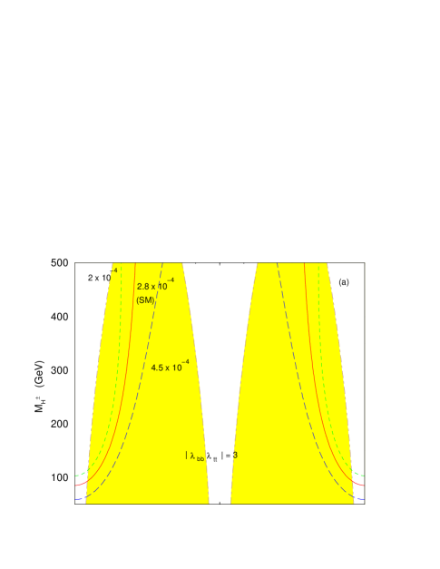
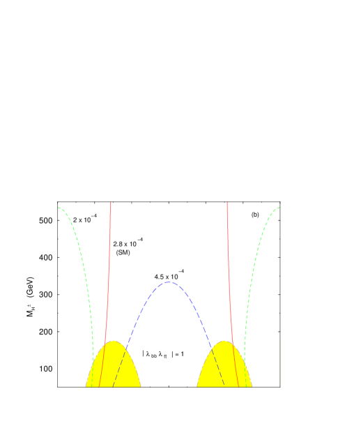
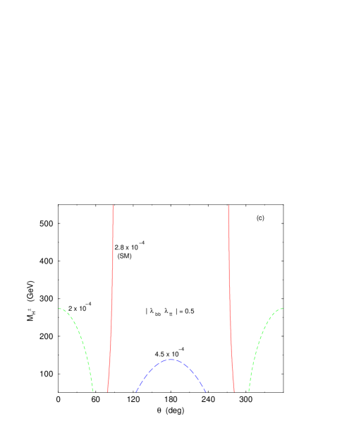
Figure 1: Contour plot of the branching ratio $b\rightarrow s\gamma$ versus $M_{H}^{\pm}$ and the phase of $\lambda_{tt}\lambda_{bb}$ for various values of $|\lambda_{tt}\lambda_{bb}|=3,1,0.5$. The shaded areas are excluded by the NEDM constraint $|d_{n}|<10^{-25}$ e$\cdot$cm.

Since the term proportional to $\lambda_{tt}\lambda_{bb}$ is, in general, complex we let $\lambda_{tt}\lambda_{bb}=|\lambda_{tt}\lambda_{bb}|e^{i\theta}$. We show the contours of the branching ratio in the plane of $\theta$ and $M_{H^{\pm}}$ for $|\lambda_{tt}\lambda_{bb}|=3,1,0.5$ in Fig. 1 (a), (b), and (c), respectively. The contours are symmetric about $\theta=180^{\circ}$. The contours are $B=(2,2.8,4.5)\times 10^{-4}$, which correspond to 95%CL lower limit, the SM value, and the 95%CL upper limit. The value of $|\lambda_{bb}|$ is set at 50 as preferred in the $R_{b}$ constraint that will be shown in the next section. The corresponding values of $|\lambda_{tt}|$ are $0.06,0.02$, and $0.01$, which satisfy the constraint from the $B^{0}-\overline{B^{0}}$ mixing, as will also be discussed in the next section. Here the term proportional to $|\lambda_{tt}|^{2}$ is not crucial because the coefficient of $|\lambda_{tt}|^{2}$ is small compared with other two terms in Eqs. (18) and (19).

The results of the conventional model II (which can be obtained from our general results by the substitution: $\lambda_{tt}\to\cot\beta$, $\lambda_{bb}\to-\tan\beta$) can be read off from Fig. 1(b) at $\theta=180^{\circ}$. The $b\to s\gamma$ data severely constrains $M_{H^{\pm}}\mathrel{\raisebox{-2.58334pt}{$\stackrel{{\scriptstyle\textstyle>}}{{\sim}}$}}350$ GeV at 95%CL level, because at $\theta=180^{\circ}$ the SM amplitude interferes entirely constructively with the charged Higgs-boson amplitude. It is obvious that at other angles the mass of the charged Higgs-boson mass is less constrained, especially, in the range $\theta=50^{\circ}-90^{\circ}$ the entire range of charged Higgs-boson mass is allowed by the $b\to s\gamma$ constraint as long as $|\lambda_{tt}\lambda_{bb}|\mathrel{\raisebox{-2.58334pt}{$\stackrel{{\scriptstyle\textstyle<}}{{\sim}}$}}1$. However, when $|\lambda_{tt}\lambda_{bb}|$ is getting larger, say 3, (see Fig. 1(a)) the allowed range of charged Higgs-boson mass becomes narrow. This is because the charged Higgs-boson amplitude becomes too large compared with the SM amplitude. On the other hand, when $|\lambda_{tt}\lambda_{bb}|$ becomes small the allowed range charged Higgs-boson mass is enlarged, as shown in Fig. 1(c). The significance of the phase angle $\theta$ is that the constraints previously on $M_{H^{\pm}}$ and $\tan\beta$ are evolved into $\theta$, $M_{H^{\pm}}$, $\lambda_{tt}$, and $\lambda_{bb}$, where we do not need to impose $|\lambda_{tt}|=1/|\lambda_{bb}|$, as in model II. The previous tight constraint on $m_{H^{\pm}}$ is now relaxed down to virtually the direct search limit of almost 60 GeV at LEPII [18].

The phase $\theta$ of $\lambda_{tt}\lambda_{bb}$ can give rise to the neutron electric dipole moment (NEDM). The physics involved can be understood as follows. First, at the electroweak scale the phase $\theta$ induces the CP violating color dipole moment (CDM) of the $b$ quark. Second, the CDM of $b$ quark evolves by renormalization to the scale at $m_{b}$ and turns into the Weinberg operator[19] (i.e. the gluonic CDM[20]) when the $b$-quark field is integrated away. Finally, this gives NEDM at the nucleon mass scale:

$$d_{n}^{g}=g_{s}^{3}(\mu)C_{g}(\mu)\langle{\cal O}_{g}(\mu)\rangle,\quad\hbox{where }{\cal O}_{g}=\hbox{$1\over 6$}f^{abc}\varepsilon^{\delta\nu\alpha\beta}G^{a}_{\alpha\beta}G^{b}_{\lambda\delta}G^{c}_{\lambda\nu}\ .$$ (26)

Weinberg suggested the hadronic scale $\mu$ to be set at the value such that $g_{s}(\mu)=4\pi/\sqrt{6}$. Instead we choose $\mu$ at the nucleon mass. The hadronic matrix element $\langle{\cal O}_{g}(\mu)\rangle$ is very uncertain. A typical estimate from the naive dimension analysis (NDA)[21] relates the matrix element to the chiral symmetry breaking scale $M_{\chi}=2\pi F_{\pi}=1.19$ GeV,

$${\cal O}_{g}={eM_{\chi}\over 4\pi}\xi_{g}(\mu)\ .$$ (27)

The parameter $\xi_{g}$ is set to be 1 in NDA, but other calculations result in different $\xi_{g}$. QCD sum rule performed by Chemtob[22] gives $\xi_{g}=0.07$. Scaling argument by Bigi and Uraltsev[23] yields a value $\xi_{g}=0.03$. We choose $\xi_{g}=0.1$ for our analysis. The Wilson coefficient of the Weinberg operator $C_{g}$ evolves according to the RG equation[24] and matches[25, 26] that induced by the CDM $C_{b}$ of the $b$ quark at the scale $m_{b}$. Our definitions of Wilson coefficients follow the notation in Ref.[26],

$$C_{g}(\mu)={1\over 32\pi^{2}}C_{b}(m_{b})\left({\alpha_{s}(m_{b})\over\alpha_{s}(m_{c})}\right)^{54\over 25}\left({\alpha_{s}(m_{c})\over\alpha_{s}(\mu)}\right)^{54\over 27}\ .$$ (28)

The CDM of the $b$ quark comes from the CP violation of the charged Higgs coupling at the electroweak scale and at the scale $m_{b}$ it is given by

$$C_{b}(m_{b})={\sqrt{2}G_{F}\over 16\pi^{2}}\hbox{Im}(\lambda_{tt}\lambda_{bb}){2\over 3}H\left(m_{t}^{2}\over M^{2}_{H^{\pm}}\right)\left({\alpha_{s}(m_{W})\over\alpha_{s}(m_{b})}\right)^{14\over 23}\ ,$$ (29)

where the function $H$ is

$$H(y)={3\over 2}{y\over(1-y)^{2}}\left(y-3-{2\log y\over 1-y}\right)\ .$$ (30)

Note that $H(1)=1$ when $M_{H^{\pm}}=m_{t}$. Numerically,

$$d^{g}_{n}=10^{-25}\hbox{e$\cdot$cm}\ \hbox{Im}(\lambda_{tt}\lambda_{bb})\left({\alpha(m_{n})\over\alpha(\mu)}\right)^{1\over 2}\left({\xi_{g}\over 0.1}\right)H\left({m_{t}^{2}\over M^{2}_{H^{\pm}}}\right)\ .$$ (31)

The experimental limit,

$$d_{n}<10^{-25}\hbox{e$\cdot$cm}\ ,$$ (32)

places an upper bound $|\hbox{Im}(\lambda_{tt}\lambda_{bb})|\mathrel{\raisebox{-2.58334pt}{$\stackrel{{\scriptstyle\textstyle<}}{{\sim}}$}}1$ on the coupling product for our choice of parameters, $\xi_{g}=0.1$, $\mu=m_{n}$ when $M_{H^{\pm}}\simeq m_{t}$. The bound is sensitive to uncertainties in $\mu$ and $\xi_{g}$, but not much in $M_{H^{\pm}}$. The function value $H$ decreases only by a factor of 1.6 as the charged Higgs mass varies from 50 GeV to 200 GeV.

In Fig. 1, the constraint on the $M_{H^{\pm}}$ versus $\theta$ is given by the shaded areas which are excluded by the NEDM measurement.

For the case of rather large $|\lambda_{tt}\lambda_{bb}|\gg 1$, the phase becomes restricted to the forward region $\theta\sim 0$ or the backward region $\pi$. However, the backward region ($\theta\sim\pi$) is not preferable for $M_{H^{\pm}}\mathrel{\raisebox{-2.58334pt}{$\stackrel{{\scriptstyle\textstyle<}}{{\sim}}$}}500$ GeV due to the constraint from $b\rightarrow s\gamma$. If the charged Higgs boson is this light with large couplings to the $b$ and $t$ quarks, the NEDM analysis requires a small phase in the forward region. On the other hand, when $|\lambda_{tt}\lambda_{bb}|<0.7$, the NEDM constraint becomes ineffective and the constraint from $b\to s\gamma$ remains useful.

Other places to look for the effects of this angle $\theta$ include other $b\to s,d$ decays, CP violation effects in $b\to s\gamma$ [11], $b\to s\ell\bar{\ell}$, and the electric dipole moments of fermions via a 2-loop mechanism [13].

On the other hand, this phase angle $\theta$ will not show up in other existing constraints like $\rho_{0}$, $R_{b}$, and flavor-mixing. The previous argument that the 2HDM only has a very narrow window left to accommodate all the constraints from $B(b\to s\gamma)$, $\rho_{0}$, $R_{b}$, and flavor-mixing is now not true because of the possible phase angle in model III that we are considering. The narrow window on $M_{H^{\pm}}$ opens up. We shall summarize the other constraints on $\lambda_{tt}$, $\lambda_{bb}$, and Higgs masses in the next section.

V. Other Constraints

Direct searches for Higgs bosons in 2HDM at LEPII [18] place the following limits on Higgs boson masses:

$$M_{h^{0}}>77\;{\rm GeV}\;,\qquad M_{A}>78\;{\rm GeV}\;,\qquad M_{H^{\pm}}>56-59\;{\rm GeV}\;,$$ (33)

where the $M_{h^{0}}$ and $M_{A}$ mass limits are obtained by combining the four LEP experiments but no combined limit on $M_{H^{\pm}}$ is available [18]. We shall then discuss other constraints from precision measurements.

V.A $K^{0}-\overline{K^{0}}$, $D^{0}-\overline{D^{0}}$, and $B^{0}-\overline{B^{0}}$

These $F^{0}-\overline{F^{0}}$ ($F=K,D,B$) flavor-mixing processes can occur via tree-level, penguin, and box diagrams in model III [10]. One particular argument against the model III is that it allows FCNC at the tree-level, but with a lot of freedom in picking the parameters $\lambda_{ij}$ it certainly survives all the present FCNC constraints. The tree-level diagrams for these $\Delta F=2$ processes can be eliminated by choosing $\lambda_{ui},\lambda_{dj}$ very small. Actually, in our study we have set $\lambda_{ij}=0\;(i\neq j)$, therefore, all tree-level FCNC diagrams are eliminated and so do the penguin diagrams. However, there are important contributions coming from the box diagrams with the charged Higgs boson. Naively, to suppress the charged Higgs contribution we need to increase the charged Higgs mass or decrease $\lambda_{tt}$. We shall obtain a set of bounds using the experimental measurement $x_{d}$ of $B^{0}-\overline{B^{0}}$ in the following ( $K^{0}-\overline{K^{0}}$ and $D^{0}-\overline{D^{0}}$ mixings are small in our model because of the mass hierarchy choice of $\hat{\xi}^{U,D}_{ij}$ in Eq. (7)).

The quantity that parameterizes the $B^{0}-\overline{B^{0}}$ mixing is

$$x_{d}\equiv\frac{\Delta m_{B}}{\Gamma_{B}}=\frac{G_{F}^{2}}{6\pi^{2}}|V_{td}^{*}|^{2}|V_{tb}|^{2}f_{B}^{2}B_{B}m_{B}\eta_{B}\tau_{B}M_{W}^{2}\left(I_{WW}+I_{WH}+I_{HH}\right)$$ (34)

where[27]

$$I_{WW} = \frac{x}{4}\biggr{[}1+\frac{3-9x}{(x-1)^{2}}+\frac{6x^{2}\log x}{(x-1)^{3}}\biggr{]}$$

$$I_{WH} = xy|\lambda_{tt}|^{2}\biggr{[}\frac{(4z-1)\log y}{2(1-y)^{2}(1-z)}-\frac{3\log x}{2(1-x)^{2}(1-z)}+\frac{x-4}{2(1-x)(1-y)}\biggr{]}$$

$$I_{HH} = \frac{xy|\lambda_{tt}|^{4}}{4}\biggr{[}\frac{1+y}{(1-y)^{2}}+\frac{2y\log y}{(1-y)^{3}}\biggr{]}\;,$$

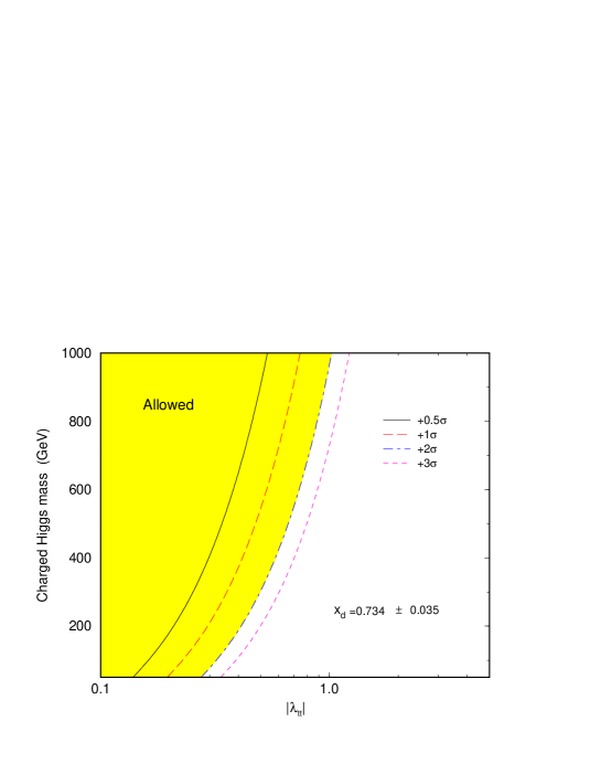
Figure 2: Contour plot of the $B^{0}-\overline{B^{0}}$ mixing parameter $x_{d}$ in the plane of $|\lambda_{tt}|$ and the charged Higgs boson mass. The experimental value is $x_{d}=0.734\pm 0.035$.

where $x=m_{t}^{2}/M_{W}^{2}$, $y=m_{t}^{2}/M_{H^{\pm}}^{2}$, $z=M_{W}^{2}/M_{H^{\pm}}^{2}$, and the running top mass $m_{t}=m_{t}(m_{t})=166$ GeV. We use these inputs [17, 16, 3]: $|V_{tb}|=1$, $f_{B}^{2}B_{B}=(0.175\;{\rm GeV})^{2}(1.4)$, $m_{B}=5.2798$ GeV, $\eta_{B}=0.55$, and $x_{d}=0.734\pm 0.035$, $\tau_{B}=1.56$ ps. Since the allowable range of $|V_{td}|$ is from 0.004 to 0.013 [17], we use a central value for $|V_{td}|$ obtained using the central value of $x_{d}$ and it gives $|V_{td}|\simeq 0.0084$ (which is the central value given in the Particle Data Book 98 [17].) We then obtain bounds on $\lambda_{tt}$ and $M_{H^{\pm}}$ by the $2\sigma$ limit of $x_{d}$ assuming the only error comes from $x_{d}$ measurement (see Fig. 2):

$$M_{H^{\pm}}\mathrel{\raisebox{-2.58334pt}{$\stackrel{{\scriptstyle\textstyle>}}{{\sim}}$}}77\;(60)\ {\rm GeV}\qquad{\rm for}\qquad|\lambda_{tt}|\mathrel{\raisebox{-2.58334pt}{$\stackrel{{\scriptstyle\textstyle<}}{{\sim}}$}}0.3\;(0.28)\;,$$ (35)

which means virtually no limit on the charged Higgs mass if $|\lambda_{tt}|\mathrel{\raisebox{-2.58334pt}{$\stackrel{{\scriptstyle\textstyle<}}{{\sim}}$}}0.28$, because the present direct search limit on charged Higgs boson is about 56–59 GeV (Eq.(33)). We have improved the results in Ref. [28, 10] because we are using an updated value of $x_{d}$. In the context of model I and II the bound is $M_{H^{\pm}}\mathrel{\raisebox{-2.58334pt}{$\stackrel{{\scriptstyle\textstyle>}}{{\sim}}$}}77(60)$ GeV for $\tan\beta\mathrel{\raisebox{-2.58334pt}{$\stackrel{{\scriptstyle\textstyle>}}{{\sim}}$}}3.3(3.6)$. For $\tan\beta$ gets close to 1, $M_{H^{\pm}}>1$ TeV.

V.B $\rho_{0}$

$\rho$ was introduced to measure the relation between the masses of $W$ and $Z$ bosons. In the SM $\rho=M_{W}^{2}/M_{Z}^{2}\cos\theta_{\rm w}=1$ at the tree-level. However, the $\rho$ parameter receives contributions from the SM corrections and from new physics. The deviation from the SM predictions is usually described by the parameter $\rho_{0}$ defined by [16]

$$\rho_{0}=\frac{M_{W}^{2}}{\rho M_{Z}^{2}\cos^{2}\theta_{\rm w}}\,,$$ (36)

where the $\rho$ in the denominator absorbs all the SM corrections, among which the most important SM correction at 1-loop level comes from the heavy top-quark:

$$\rho\simeq 1+\Delta\rho_{\rm top}=1+\frac{3G_{F}}{8\sqrt{2}\pi^{2}}\,m_{t}^{2}\,,$$ (37)

in which $\Delta\rho_{\rm top}$ is about 0.0095 for $m_{t}=173.8$ GeV. By definition $\rho_{0}\equiv 1$ in the SM. The reported value of $\rho_{0}$ is [16]

$$\rho_{0}=0.9996\stackrel{{\scriptstyle\scriptstyle+0.0017}}{{\scriptstyle-0.0013}}\;\;(2\sigma)\,.$$ (38)

In terms of new physics (2HDM here) the constraint becomes:

$$-0.0017<\Delta\rho_{\rm 2HDM}<0.0013\;.$$ (39)

In 2HDM $\rho_{0}$ receives contribution from the Higgs bosons given by, in the context of model III, [28, 29, 10]

$$\Delta\rho_{\rm 2HDM}=\frac{G_{F}}{8\sqrt{2}\pi^{2}}\biggr{[}\sin^{2}\alpha F(M_{H^{\pm}},M_{A},M_{H^{0}})+\cos^{2}\alpha F(M_{H^{\pm}},M_{A},M_{h^{0}})\biggr{]}\,,$$ (40)

where

$$F(m_{1},m_{2},m_{3}) = m_{1}^{2}-\frac{m_{1}^{2}m_{2}^{2}}{m_{1}^{2}-m_{2}^{2}}\log\left(\frac{m_{1}^{2}}{m_{2}^{2}}\right)$$

$$-\frac{m_{1}^{2}m_{3}^{2}}{m_{1}^{2}-m_{3}^{2}}\log\left(\frac{m_{1}^{2}}{m_{3}^{2}}\right)+\frac{m_{2}^{2}m_{3}^{2}}{m_{2}^{2}-m_{3}^{2}}\log\left(\frac{m_{3}^{2}}{m_{3}^{2}}\right)\;.$$

Since $\rho_{0}$ is constrained to be around 1 we have to minimize the contributions of $\Delta\rho_{\rm 2HDM}$. Without loss of generosity we set $\alpha=0$, which means that the heavier neutral Higgs $H^{0}$ decouples and the first Higgs doublet can be identified as the SM Higgs doublet, while the second Higgs doublet is the source of new physics. The leading behavior of $\Delta\rho_{\rm 2HDM}$ scale as $M_{H^{\pm}}^{2}$ and, therefore, the constraint of $\rho_{0}$ in Eq. (38) puts an upper bound on $M_{H^{\pm}}$. Actually, if the charged Higgs mass $M_{H^{\pm}}$ is between $M_{A}$ and $M_{h^{0}}$ the $\Delta\rho_{\rm 2HDM}$ is negative. However, this is not the favorite scenario because in the case of $R_{b}$ the experimental result prefers $M_{A}\simeq M_{h^{0}}\approx 80-120$ GeV, that will be discussed in the next subsection. In this case $M_{A}\simeq M_{h^{0}}$, $\Delta\rho_{\rm 2HDM}$ is positive and, therefore, we want to keep it small. Using Eq. (40) for $M_{A}\simeq M_{h^{0}}=80-120$ GeV, the charged Higgs mass is constrained to be

$$M_{H^{\pm}}\mathrel{\raisebox{-2.58334pt}{$\stackrel{{\scriptstyle\textstyle<}}{{\sim}}$}}180-220\;{\rm GeV}\;.$$ (41)

V.C $R_{b}$

$R_{b}$ was about $+3.7\sigma$ above the SM value a few years ago, but now the deviation is reduced to $+1\sigma$ after almost all LEP data have been analyzed [16]. $R_{b}^{\rm exp}$ still places a constraint on the 2HDM, though it is much less severe than before. This is because only a narrow window exists in the neutral Higgs bosons that does not decrease $R_{b}$ while the charged-Higgs boson always decreases $R_{b}$. We shall divide the discussion into two parts: neutral-Higgs contribution and charged-Higgs contribution.

According to Ref. [29] the contribution from the neutral Higgs boson is positive in a narrow window of $20\;{\rm GeV}<M_{A}\simeq M_{h^{0}}<120$ GeV and is negative otherwise. Since the charged Higgs boson contribution always decreases $R_{b}$, it makes more sense to require the neutral Higgs contribution to be positive. Here we adapt the formulas in Ref. [29] to model III. First, the contribution from the neutral Higgs bosons only depends on $|\lambda_{bb}|$ and the masses of the neutral Higgs bosons. Again without loss of generosity, we set the scalar Higgs-boson mixing angle $\alpha=0$ in order to decouple the heavier $H^{0}$. We show the resultant $R_{b}$ due to the presence of the neutral Higgs bosons in Fig. 3(a) for $|\lambda_{bb}|=30,50,70$, where $R_{b}^{\rm SM}=0.2158$, $R_{b}^{\rm exp}=0.21656\pm 0.00074$ [16], and the $1\sigma$ is taken to be the standard deviation of the experimental result. In Fig. 3(a) the horizontal lines represent the $R_{b}^{\rm SM}$, $+1\sigma$, and $+2\sigma$ values. The $R_{b}^{\rm exp}$ is almost at the $+1\sigma$ line. If we allow only $1\sigma$ value below $R_{b}^{\rm exp}$, we need $M_{h^{0}}\approx M_{A}\approx 80-120$ GeV with a fairly large $|\lambda_{bb}|$. For $|\lambda_{bb}|$ as large as 70 the enhancement can be as large as $+1\sigma$ at $M_{H^{\pm}}=80$ GeV. On the other hand, if we allow $2\sigma$ below $R_{b}^{\rm exp}$, then we can have all the range of $M_{h^{0}}\approx M_{A}>80$ GeV, as can be seen in Fig. 3(a). At any rate, the preferred scenario is $M_{h^{0}}\approx M_{A}=80-120$ GeV with a fairly large $|\lambda_{bb}|$. How large $|\lambda_{bb}|$ should be? It depends on the charged Higgs contribution as well.

Since the charged Higgs-boson contribution is always negative, we want to make it as small as possible. This contribution depends on $|\lambda_{tt}|$, $|\lambda_{bb}|$, and $M_{H^{\pm}}$. The effect on $R_{b}$ due to the presence of the charged Higgs boson is shown in Fig. 3(b) for $|\lambda_{bb}|=30,50,70$ and $|\lambda_{tt}|=0.05$. In Fig. 3(b) the horizontal lines represent the $R_{b}^{\rm SM}$ and $\pm 1\sigma$. The $R_{b}^{\rm exp}$ is very close to $+1\sigma$ line. It is clear from the graph that because we do not want the charged Higgs contribution to reduce $R_{b}^{\rm SM}$ by more than $1\sigma$, we require $M_{H^{\pm}}\mathrel{\raisebox{-2.58334pt}{$\stackrel{{\scriptstyle\textstyle>}}{{\sim}}$}}60\;(220)$ GeV for $|\lambda_{bb}|=50\;(70)$.

Since $R_{b}^{\rm exp}$ is only $+1\sigma$ away from $R_{b}^{\rm SM}$, it is not necessary to keep the narrow window of $M_{A}$ and $M_{h^{0}}$ if we allow $2\sigma$ below the experimental data. In this case, $M_{h^{0}}$ and $M_{A}$ can be widened to much larger masses, and so the $\rho_{0}$ constraint on the ceiling of the charged Higgs mass will also be relaxed. However, $M_{H^{\pm}}$ cannot be too small otherwise $R_{b}$ will be decreased to an unacceptable value.

Summarizing this section the constraints by $B^{0}-\overline{B^{0}}$ mixing, $\rho_{0}$, and $R_{b}$ give the following preferred scenario:

1. $M_{A}\simeq M_{h^{0}}=80-120$ GeV;

2. $|\lambda_{bb}|\simeq 50$;

3. $|\lambda_{tt}|\mathrel{\raisebox{-2.58334pt}{$\stackrel{{\scriptstyle\textstyle<}}{{\sim}}$}}0.3$;

4. $80$ GeV $\mathrel{\raisebox{-2.58334pt}{$\stackrel{{\scriptstyle\textstyle<}}{{\sim}}$}}M_{H^{\pm}}\mathrel{\raisebox{-2.58334pt}{$\stackrel{{\scriptstyle\textstyle<}}{{\sim}}$}}200$ GeV.

VI. Conclusions

We have demonstrated in model III of the general two-Higgs-doublet model the charged-Higgs-fermion couplings can be complex, even in the simplified case of no tree-level FCNC couplings. The phase angle in the complex charged-Higgs-fermion coupling determines the interference between the standard model amplitude and the charged-Higgs amplitude in the process of $b\to s\gamma$. We found that for $|\lambda_{bb}\lambda_{tt}|\simeq 1$ there is a large range of the phase angle ($\theta\approx 50^{\circ}-90^{\circ}$ and $270^{\circ}-310^{\circ}$) such that the rate of $b\to s\gamma$ is within the experimental value for all range of $M_{H^{\pm}}$. In other words, the previous tight constraints on $M_{H^{\pm}}$ from the CLEO $b\to s\gamma$ rate is relaxed, depending on this phase angle. In addition, we also examined the effect of this phase angle on the neutron electric dipole moment and discussed other experimental constraints on model III. The necessary constraints are already listed at the end of the last section. Here we offer the following comments:

1. The phase angle induces a CP-violating chromoelectric dipole moment of the $b$-quark, which leads to a substantial enhancement in neutron electric dipole moment. The experimental upper limit on neutron electric dipole moment thus places a upper bound on the couplings: $|\lambda_{tt}\lambda_{bb}|\sin\theta\mathrel{\raisebox{-2.58334pt}{$\stackrel{{\scriptstyle\textstyle<}}{{\sim}}$}}0.8$ for $M_{H^{\pm}}\approx 100$ GeV. This bound has large uncertainties due to the hadronic matrix element of the neutron and the factorization scale.

2. The phase angle will also cause other CP-violating effects in other processes, e.g., the decay rate difference between $b\to s\gamma$ and $\bar{b}\to\bar{s}\gamma$ [11], and in lepton asymmetries of $b\to s\ell^{+}\ell^{-}$. These processes will soon be measured at the future $B$ factories.

3. Other experimental measurements, like $F^{0}-\overline{F^{0}}$ mixing, $\rho_{0}$, and $R_{b}$, constrain only the magnitude of the couplings and the Higgs-boson masses but not the phase angle.

4. The $B^{0}-\overline{B^{0}}$ mixing measurement can only constrain the charged-Higgs mass and $|\lambda_{tt}|$ loosely because the mixing parameter $x_{d}$ depends on $|V_{td}|$, which is not yet well measured. Other uncertainties come from the hadronic factors: $f_{B}$, $B_{B}$, and $\eta_{B}$. Actually, the mixing parameter $x_{d}$ is often used to determine $|V_{td}|$.

5. As we have mentioned, if $R_{b}^{\rm SM}$ gets closer to the SM value the constraint on the neutral Higgs-boson masses: $M_{A}$ and $M_{h^{0}}=80-120$ GeV will go away completely. On the other hand, the charged-Higgs boson mass is still required to be larger than about 60 GeV (for $|\lambda_{bb}|=50$) in order not to decrease $R_{b}$ significantly.

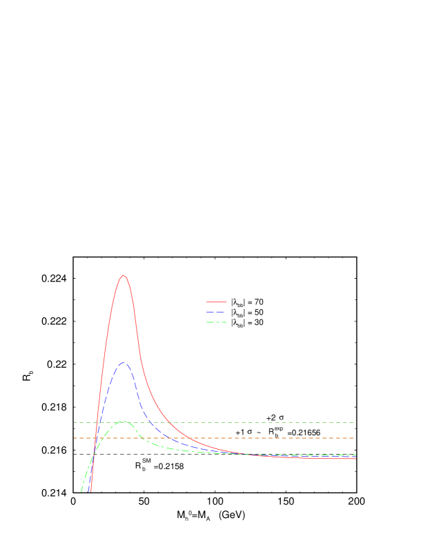
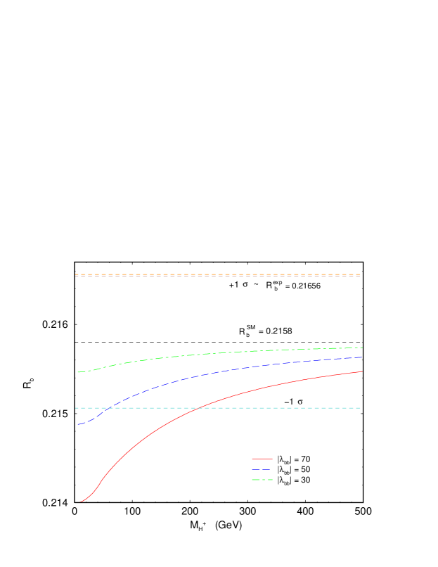
Figure 3: The $R_{b}\equiv\Gamma(Z\to b\bar{b})/\Gamma_{\rm had}$ due to the presence of (a) the neutral Higgs bosons, $M_{A}\simeq M_{h^{0}}$ and (b) the charged Higgs boson.

References

- [1] The Higgs Hunter’s Guide by J. Gunion et al., Addison-Wesley, New York, 1990.
- [2] S. Glashow and S. Weinberg, Phys. Rev. D15, 1958 (1977).
-
[3]
G. Buchalla, A. Buras, and M. Lautenbacher,
Rev. Mod. Phys. 68, 1125 (1996);
A.J. Buras, M. Misiak, Münz, and S. Pokorski, Nucl. Phys. 424, 374 (1994). - [4] K. Chetyrkin, M. Misiak, and M. Munz, Phys. Lett. B400, 206 (1997); Erratum-ibid. B425, 414 (1998); M. Ciuchini, G. Degrassi, P. Gambino, and G.F. Giudice, Nucl. Phys. B527, 21 (1998);A. Kagan, M. Neubert, e-Print Archive: hep-ph/9805303.
- [5] M.S. Alam et al. (CLEO Coll.), Phys. Rev. Lett. 74, 2884 (1995).
- [6] talk by R. Briere, CLEO-CONF-98-17, ICHEP98-1011, in Proceedings of ICHEP98, Vancouver, Canada, July 1998; and in talk by J. Alexander, in Proceedings of ICHEP98, Vancouver, Canada, July 1998.
- [7] ALEPH Coll. (R. Barate et al.), Phys. Lett. B429, 169 (1998).
-
[8]
J.L. Hewett Phys. Rev. Lett. 70, 1045 (1993);
V. Barger, M.S. Berger, and R.J.N. Phillips, Phys. Rev. Lett. 70, 1368 (1993). -
[9]
T.P. Cheng and M. Sher, Phys. Rev. D35, 3484 (1987);
D44, 1461 (1991);
W.S. Hou, Phys. Lett. B296 179 (1992);
A. Antaramian, L. Hall, and A. Rasin, Phys. Rev. Lett. 69, 1871 (1992);
L. Hall and S. Weinberg, Phys. Rev. D48, 979 (1993);
M.J. Savage, Phys. Lett. B266, 135 (1991). - [10] D. Atwood, L. Reina, and A. Soni, Phys. Rev. D55, 3156 (1997).
- [11] L. Wolfenstein and Y.L. Wu, Phys. Rev. Lett. 73, 2809 (1994).
- [12] M. Kobayashi and M. Maskawa, Prog. Theor. Phys. 49, 652 (1973).
- [13] D. Bowser-Chao, W.-Y. Keung, and D. Chang, Phys. Rev. Lett.79, 1988 (1997).
- [14] B. Grinstein, R. Springer, and M. Wise, Nucl. Phys. B339, 269 (1990).
- [15] T. Inami and C.S. Lim, Prog. Th. Phys. 65, 297 (1981); erratum, ibidem,1772.
- [16] P. Langacker and J. Erler, hep-ph/9809352, to appear in Proceedings of the 5th International WEIN Symposium: A Conference on Physics Beyond the Standard Model (WEIN 98), Sante Fe, NM, June 14–21, 1998.
- [17] Review of Particle Physics by Particle Data Group, Euro. Phys. J. C3, 1 (1998).
- [18] Talk by K. Desch, “Beyond SM Higgs Search at LEP”, at ICHEP98, Vancouver, Canada, July 1998.
- [19] S. Weinberg, Phys. Rev. Lett. 63, 2333 (1989).
- [20] E. Braaten, C.S. Li, and T.C. Yuan, Phys. Rev. D 42, 276 (1990).
- [21] A. Manohar and H. Georgi, Nucl. Phys. B234, 189 (1984); H. Georgi and L. Randall, Nucl. Phys. B276, 241 (1986).
- [22] M. Chemtob, Phys. Rev. D 45 1649, (1992).
- [23] I.I. Bigi and N.G. Uraltsev, Nucl. Phys. B353, 321 (1991).
- [24] E. Braaten, C.S. Li, and T.C. Yuan, Phys. Rev. Rev. 64, 1709 (1990).
- [25] G. Boyd, A. Gupta, S. Trivedi, and M. Wise, Phys. Lett. B241, 584 (1990).
- [26] D. Chang, W.–Y. Keung, C.S. Li, and T.C. Yuan, Phys. Lett. 241 589, (1990).
- [27] L.F. Abbott, P. Sikivie, and M. B. Wise, Phys. Rev. D 21, 1393 (1980); G.G. Athanasiu, P.J. Franzini, and F.J. Gilman, S.L. Glashow and E.E. Jenkins, Phys. Lett. 196B, 233 (1987); Phys. Rev. D 32, 3010 (1985); C.Q. Geng and J.N. Ng, Phys. Rev. D 38, 2857 (1988).
- [28] A. Grant, Phys. Rev. D51, 207 (1995).
- [29] A. Denner et al., Z. Phys. C51, 695 (1991).