Higgs– and Goldstone bosons–mediated
long range forces

Abstract

In certain mild extensions of the Standard Model, spin-independent long range forces can arise by exchange of two very light pseudoscalar spin–$0$ bosons. In particular, we have in mind models in which these bosons do not have direct tree level couplings to ordinary fermions. Using the dispersion theoretical method, we find a $1/r^{3}$ behaviour of the potential for the exchange of very light pseudoscalars and a $1/r^{7}$ dependence if the pseudoscalars are true massless Goldstone bosons.

I Introduction

Most studies and investigations on long range forces have always centered, for obvious reasons, around the electromagnetic and gravitational interaction. However, starting with the very early example of the Casimir–Polder long range force [1], over the Feinberg–Sucher force [2] mediated by two neutrinos (see Fig.1) and finally going to recent developments in supersymmetry and superstrings [3], there has been a continuous interest in effects and detection of exotic long range forces [4]. The actual applicability or relevance of these forces is, of course, different from case to case. For instance, the Casimir–Polder force is, in principle, of electromagnetic origin. It arises as a consequence of photon exchange between polarizable neutral systems and the resulting potential has a $1/r^{7}$ dependence at long distances. Although the Casimir–Polder force has been recently detected in a laboratory experiment [5], the neutrino mediated (i.e. involving weak interaction couplings) Feinberg–Sucher force is too weak to be of any significance in Earth–based experiments. If at all, a suitable arena for this force would be of astrophysical and/or cosmological dimension (see for instance in this respect [6] and references in [7]). The result of Feinberg and Sucher has been recently extended to also account for the exchange of very light Dirac [8] and Majorana [9] neutrinos. Temperature–dependent corrections including the exchange of thermalized neutrinos at finite temperature, like the relic cosmic neutrinos at $T^{-1}\sim 1mm$, have been calculated in [10, 7]. Finally let us mention that extensions of the Standard Model can allow, in principle, for a variety of different long range forces [4], mediated, for instance by very light or massless scalars or pseudoscalars [11]. The former force acting between neutrinos themselves has been discussed e.g. in [12]. The potential due to the exchange of two pseudoscalar particles (box–diagrams) was computed in [13, 14]. Furthermore, new exotic long range forces can appear also in the context of gauge mediated supersymmetry breaking and in superstring theories [3]. The implications of a new long range force due to an extra $U(1)$ gauge group have been discussed recently by Fayet in [15].

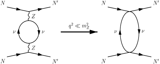
FIG. 1.: One of the diagrams in the S.M. giving rise to the two neutrino force in four-Fermi effective theory.

Should neutrinos be the only massless or very light particles in spectrum of the theory, then the Feinberg–Sucher result would be the only possible exotic long range force, regardless of the model. This is clear since all long range forces (including the electromagnetic and gravitational interaction) arise as a consequence of an exchange of very light quanta. However, as mentioned above many extensions of the Standard Model also predict very light pseudoscalars. Usually diagrams involving two such pseudoscalars will then result in a spin–independent long range force between standard fermions [13, 14]. Recall that a exchange of a single pseudoscalar between fermions gives a spin–dependent result for the potential [4]. Indeed, a covariant calculation with two pseudoscalars exchange has been recently performed in [14] in the context of a generic theory where the coupling of the pseudoscalar $\phi$ to fermions is taken either as $\phi\bar{\psi}\gamma_{5}\psi$ or, alternatively, as the derivative version $(\partial_{\mu}\phi)\bar{\psi}\gamma_{5}\gamma^{\mu}\psi$, in the latter case $\phi$ can represent a generic Goldstone boson. In the first case the authors obtain the a $1/r^{3}$ dependence of the potential whereas the double exchange of Goldstone bosons yields a more drastic fall–off, viz $1/r^{5}$. However, very often, i.e. in a wide class of models, these pseudoscalars do not couple to standard fermions (often not even to gauge bosons) on account of some symmetry arguments (see appendix where one such model is briefly sketched). However they do always have a tree level coupling to Higgs–scalar particles of the theory. Indeed, it is difficult to imagine a reasonable symmetry argument which would forbid such couplings. We now assume that the scalars themselves couple to standard fermions, which is the case in most models. If so, then the diagram in Fig. 2 displays a very nice analogy to the diagram responsible for the Feinberg–Sucher force (see Fig. 1). Indeed, we have replaced only fermions by bosons when comparing Fig. 1 with Fig. 2. Of course, one expects a different $r$ dependence of the potential arising from the two diagrams due to different dimensionality of the the coupling constants. If the pseudoscalars have both couplings, to the fermions as well as to the Higgses, the result of [14] and our paper should then be added. Since the coupling of the scalar Higgs to fermions is usually proportional to the mass of the fermion, one may suspect that the box–diagrams using the direct pseudoscalar–fermion coupling are more important. In general this is model–dependent, but we can safely state here that the pseudoscalar fermion coupling constant is also ‘experimentally’ restricted by arguments of energy loss in stars where one assumes that the bulk of energy of the star is carried away by the standard mechanism in form of photons and neutrinos [16].

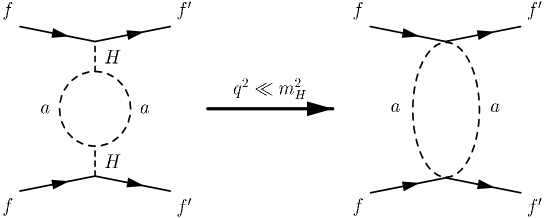
FIG. 2.: Pseudoscalar mediated long range force without direct fermion coupling.

If we assume that the pseudoscalar is a Goldstone boson, a connection to the $U(1)$–forces considered in [15] can be possibly made as the latter display a ‘Goldstone–like’ behaviour as we approach with the $U(1)$ coupling to zero [15].

The paper is organized as follows. In section 2 we calculate, using dispersion theoretical methods [17], the long range force due to the diagram in Fig. 2 where we assume that the coupling between the Higgs ($H$) and the very light pseudoscalar ($a$) is linear and of the form $Haa$. We also briefly touch some issues concerning a possible temperature dependence of the potential. In the subsequent section we change the linear coupling to a derivative version of the form $H(\partial_{\mu}a)(\partial^{\mu}a)$. In section 4 we discuss the particular case of Goldstone bosons exchange. In section 5 we summarize our results.

II Long range forces due to pseudoscalar-pseudoscalar-scalar non-derivative couplings

The dispersion theoretical technique of calculating long range forces in quantum field theory is reviewed in detail in [17]. This method is especially suitable to cope with higher order diagrams and relativistic effects and its implementation to compute the neutrino pair exchange force is straightforward [2]. The results agree with the computations done in [18] by performing the Fourier transform of the associated Feynman amplitude in momentum space (this latter strategy is only applicable in general when there is no lower order long range force and relativistic corrections are negligible).

According to the rules of the dispersion theoretical method we must compute the following Laplace transform (we restrict here ourselves to central forces which depend only on the distance $r\equiv|{\mathbf{r}}|$ between the two particles):

$$V(r)={-i\over 8\pi^{2}r}\;\int^{\infty}_{4m_{a}^{2}}{\!dt\>[{\cal M}]_{t}\,\exp(-\sqrt{t}\,r)}$$ (1)

where the integration variable $t$ stands for the usual Mandelstam variable which equals the four–momentum transfer squared, $q^{2}$. Here, $[{\cal M}]_{t}$ denotes the discontinuity of the Feynman amplitude (i.e. the absorptive part of the same) across the cut in the real $t$ axis and is best computed by taking advantage of the analyticity and generalized unitarity properties leading to the Cutkosky rules [17].

Let us now consider the case of some generic interaction terms of the form

$${\cal L}_{int}=g_{{}_{Hff}}\bar{f}fH,\,\,\,\,\,{\cal L}^{\prime}_{int}=g_{{}_{Haa}}aaH$$ (2)

where $f$ are standard fermions, $H$ is the heavy Higgs with mass $m_{H}$ and $a$ is the very light pseudoscalar with mass $m_{a}$. We can essentially neglect here possible quartic couplings of the form $H^{2}a^{2}$ as self–energy corrections due to this quartic coupling would only eventually give rise to contact interactions.

It is convenient to define global coupling constants as

$$G\equiv{g_{{}_{Hff}}g_{{}_{Haa}}\over m_{H}^{2}},\,\,\,\,\,G^{\prime}\equiv{g_{{}_{Hf^{\prime}f^{\prime}}}g_{{}_{Haa}}\over m_{H}^{2}}$$ (3)

which capture the constants of the four vertices and the two Higgs propagators in Fig.2. For future reference we draw the reader’s attention to the fact that we have expanded the Higgs propagators in $q^{2}$ and kept only the zeroth order of this expansion; this then gives the $m_{H}^{2}$ in the denominators of $G$ and $G^{\prime}$ in (3). The full matrix element of the diagram in Fig.2 is given by

$${\cal M}=-2\,i\,GG^{\prime}\>\Gamma\>\left[\bar{u}(p_{1}^{\prime})u(p_{1})\;\bar{u}(p_{2}^{\prime})u(p_{2})\right].$$ (4)

The one–loop integral is represented above by $\Gamma$ i.e.

$$\Gamma \equiv \int{\!\!d^{4}k\over(2\pi)^{4}}{i\over k^{2}-m_{a}^{2}+i\epsilon}\,{i\over\bar{k}^{2}-m_{a}^{2}+i\epsilon}$$ (5)

$$\bar{k}=k-q, \quad q=p_{1}-p_{1}^{\prime}=p_{2}^{\prime}-p_{2},\quad\quad q^{2}=t\>.$$ (6)

We assume also the non–relativistic limit in which we have $\bar{u}(p_{1}^{\prime})u(p_{1})=\bar{u}(p_{2}^{\prime})u(p_{2})\simeq 1$. Using the prescriptions arising from generalized unitarity, which amount to the replacement,

$$\frac{1}{k^{2}-m_{a}^{2}+i\epsilon}\;\;\longrightarrow-2\pi i\>\delta(k^{2}-m_{a}^{2})\>\Theta(k^{0}),$$ (7)

we obtain for the discontinuity

$$[\Gamma]_{t} = \frac{1}{(2\pi)^{2}}\int{\!\!{d^{4}k\over(2\pi)^{4}}\>\delta(k^{2}-m_{a}^{2})\>\delta(\bar{k}^{2}-m_{a}^{2})\>\theta(k^{0})\>\theta(\bar{k}^{0})}$$ (8)

$$= {1\over 8\pi}\>\sqrt{1-\frac{4m_{a}^{2}}{t}}.$$ (9)

Obviously we have $[{\cal M}]_{t}=-2\,i\,GG^{\prime}\>[\Gamma]_{t}$ which has to be inserted into (1) to compute the final expression of the potential:

$$V(r) = -\frac{GG^{\prime}}{32\pi^{3}r}\;\int^{\infty}_{4m_{a}^{2}}{\!dt\>\sqrt{1-\frac{4m_{a}^{2}}{t}}\;\exp(-\sqrt{t}\,r)}$$ (10)

$$= -\frac{GG^{\prime}m_{a}}{8\pi^{3}r^{2}}\;K_{1}(2m_{a}r)$$ (11)

where $K_{1}$ is a modified Bessel function. To show that (10), for a very small mass $m_{a}$, yields indeed a long range potential, let us take the limit $m_{a}\to 0$ in (10) (equivalent to $rm_{a}<<1$). For the leading order of the expansion we get

$$V(r)\simeq-\frac{GG^{\prime}}{16\pi^{3}r^{3}}.$$ (12)

For comparison we quote below the Feinberg–Sucher result for massless neutrinos [2]

$$V_{FS}(r)={G^{2}_{F}g_{v}g_{v^{\prime}}\over 4\pi^{3}r^{5}}$$ (13)

where $G_{F}$ is the Fermi and $g_{v}$ and $g_{v^{\prime}}$ weak vector coupling constants. Note that, in contrast to (12), the Feinberg–Sucher force (13) is repulsive. This difference between these two forces is due to an extra minus sign for the fermion–loop in (13).

We would like to touch at this point briefly upon finite temperature corrections to (10) and (12). In doing so we will follow mainly [10] and [7] to which we refer the reader for more details on this subject. At finite temperature $T$ the spin–$0$ boson propagator $S_{T}(k)$ takes the form

$$S_{T}(k)={1\over k^{2}-m_{a}^{2}+i\epsilon}-2i\pi\>\delta(k^{2}-m_{a}^{2})\>n(T),$$ (14)

where $n(T)$ is the particle distribution function with the chemical potential already set to zero. As noted explicitly in [10], the propagator (14) is sufficient to calculate the problem at hand.

We will restrict ourselves to Boltzmann distributions,

$$n(T)=\exp\left[(-E_{k})/T\right],$$ (15)

in which $E_{k}$ is the energy. To calculate the potential itself we use now the method of Fourier–transforming the momentum amplitude i.e.

$$V_{T}(r)=\int{\!\!{d^{3}{\mathbf{Q}}\over(2\pi)^{3}}\;\exp(i{\mathbf{Q}}{\mathbf{r}})\>{\cal M}_{T}({\mathbf{Q}})}={1\over 2\pi^{2}r}\int^{\infty}_{0}\!dQ\>Q\>{\cal M}_{T}(Q)\>\sin Qr$$ (16)

where in the static limit we have $q\simeq(0,{\mathbf{Q}})$ and in the second equality we have defined $Q=|{\mathbf{Q}}|$ and $r=|{\mathbf{r}}|$. The second expression in (16) holds for potentials which depend only on $r$. As before, we can write effectively ${\cal M}_{T}\simeq-2iGG^{\prime}\>\Gamma_{T}$ such that $\Gamma_{T}$ is the one loop–integral involving two ‘cross’ products of two propagators, one the standard vacuum part and the other thermal part, viz

$$\Gamma_{T}=\int{\!\!{d^{4}k\over(2\pi)^{4}}\>2i\pi\>\delta(k^{2}-m_{a}^{2})\>n(T)\left({1\over(k+q)^{2}-m_{a}^{2}}+{1\over(k-q)^{2}-m_{a}^{2}}\right)}.$$ (17)

$\Gamma_{T}$ can be further evaluated to be

$$\Gamma_{T}={4i\over(2\pi)^{2}}\>\int_{0}^{\infty}{\!\!{dkk^{2}\over\sqrt{k^{2}+m_{a}^{2}}}\exp(-\sqrt{k^{2}+m_{a}^{2}}/T)\int_{-1}^{1}{dz{1\over 4k^{2}z^{2}-Q^{2}}}}$$ (18)

where now $k=|{\mathbf{k}}|$. Recalling that ${\cal M}_{T}=-2iGG^{\prime}\>\Gamma_{T}$ and inserting this into (16) and subsequently performing the integration first over $Q$ and then over $z$ we get

$$V_{T}(r) = -{GG^{\prime}\over 4\pi^{3}}{1\over r^{2}}\>\int_{0}^{\infty}{\!{k\,dk\over\sqrt{k^{2}+m_{a}^{2}}}\exp\left(\sqrt{k^{2}+m_{a}^{2}}/T\right)\>\sin(2kr)}$$ (19)

$$= -{GG^{\prime}\over 2\pi^{2}}{1\over r}{Tm_{a}\over\sqrt{1+(2rT)^{2}}}\;K_{1}\!\left(\displaystyle{{m_{a}\over T}}\sqrt{1+(2rT)^{2}}\right).$$ (20)

Equation (19) is the finite temperature correction to (10). It is instructive at this stage to examine different limits of (19). First, let us go with the mass $m_{a}$ to zero as done in (12) for the vacuum contribution. We get the simple result

$$V_{T}(r)\simeq-{GG^{\prime}\over 2\pi^{3}}{1\over r}{T^{2}\over 1+(2rT)^{2}}.$$ (21)

Using the last limit (i.e. $m_{a}\to 0$) we can also investigate the range $r\gg T^{-1}$. In this range (21) can be expanded to give

$$V_{T}(r)\simeq-{GG^{\prime}\over 8\pi^{3}r^{3}}.$$ (22)

Remaining in this long distance range, as compared to the temperature inverse, we can add now to the vacuum part (12) equation (22) to arrive at the complete answer for the potential

$$V_{tot}(r)=V_{T}(r)+V(r)\simeq-{3\over 16}{GG^{\prime}\over\pi^{3}r^{3}}$$ (23)

This last result is particularly interesting when we compare it with the corresponding result in the context of the two neutrino force, calculated at zero and finite temperature [7]. In the neutrino case the total sum consisting of the vacuum part and the finite temperature contribution (i.e. an equation corresponding to (23)) switches the sign of the force in the range $r\gg T^{-1}$, a repulsive force becomes attractive in the presence of relic neutrinos [7]. This is a quite interesting result which sheds new light on the Feinberg–Sucher force. The reason why a similar reversal does not take place in the two boson force (cf. eq.(23)) (i.e. why this attractive force does not become repulsive when we add temperature corrections) is due to the fact that the relative sign between the vacuum part of the propagator and the thermal part is plus in the boson propagator (cf. eq. (14)) whereas it is minus for fermions [19].

Although the temperature of the very light pseudoscalars at the present epoch, provided of course these pseudoscalars exist, is model dependent, it should be comparable (at least in the order of magnitude) to the temperature of relic Axions [20] or Majorons [21].

III The case of derivative couplings

In this section we will also compute the dispersion force arising from Fig.2, considering however a different coupling scheme between the heavy Higgs and the light pseudoscalars. For the relevant Lagrangian interaction we take now [22]

$${\cal L}^{\prime\prime}_{int}=\tilde{g}_{{}_{Haa}}H(\partial^{\mu}a)(\partial_{\mu}a).$$ (24)

To simplify things, we will also start right from the beginning considering massless pseudoscalars (instead of taking the limit $m_{a}\to 0$ at the end of the calculation). We define also over–all couplings in analogy to (3)

$$\tilde{G}\equiv{g_{{}_{Hff}}\tilde{g}_{{}_{Haa}}\over m_{H}^{2}},\,\,\,\,\,\tilde{G}^{\prime}\equiv{g_{{}_{Hf^{\prime}f^{\prime}}}\tilde{g}_{{}_{Haa}}\over m_{H}^{2}}.$$ (25)

As in the preceding section we start with the dispersion theoretical definition of the potential i.e. eq. (1) where we denote now the matrix element by $\tilde{{\cal M}}$ given by

$$\tilde{{\cal M}} \simeq -2i\tilde{G}\tilde{G}^{\prime}\cdot\tilde{\Gamma}$$ (26)

$$\tilde{\Gamma} = \int{\!\!\frac{d^{4}k}{(2\pi)^{4}}\,\frac{i}{k^{2}}\,\frac{i}{\bar{k}^{2}}\,(k\cdot\bar{k})^{2}}$$ (27)

where as before $\bar{k}=q-k$. The rest of the calculation follows essentially the same line as in section 2. First we have to calculate the discontinuity $[\tilde{{\cal M}}]_{t}\propto[\tilde{\Gamma}]_{t}$ and insert the result into equation (1). For the discontinuity we obtain

$$\left[\tilde{\Gamma}\right]_{t} = \frac{q^{\mu}q^{\nu}}{(2\pi)^{2}}\int{d^{4}k\;\delta(k^{2})\delta(\bar{k}^{2})\>k_{\mu}k_{\nu}}$$ (28)

$$= \frac{q^{\mu}q^{\nu}}{(2\pi)^{2}}\frac{\pi}{2}\left[\frac{1}{3}\left(q_{\mu}q_{\nu}-\frac{1}{4}g_{\mu\nu}q^{2}\right)\right]$$ (29)

$$= \frac{t^{2}}{32\pi}$$ (30)

with $q^{2}=t$ as usual. It remains calculating the integral transform of this discontinuity. To distinguish the potential from the results in the preceding section we will call the potential due to two pseudoscalar exchange arising from the interaction (24), $\tilde{V}$. For the latter we get

$$\tilde{V}(r) = -\frac{\tilde{G}\tilde{G}^{\prime}}{128\pi^{3}r}\>\int_{0}^{\infty}{\!\!dt\>\exp(-\sqrt{t}\>r)\>t^{2}}$$ (31)

$$= -\frac{15\tilde{G}\tilde{G}^{\prime}}{8\pi^{3}r^{7}}.$$ (32)

If we compare this expression with the potential (12) it becomes clear that it is the $q^{4}=t^{2}$ dependence of $[\Gamma]_{t}$ which gives here the steep fall–off proportional to $1/r^{7}$. In (12) the corresponding integrand i.e. $[\Gamma]_{t}$ was simply a constant (for $m_{a}=0$) giving rise to a milder $1/r^{3}$ dependence.

In principle, one could now also calculate temperature–dependent effects as we have done in section 2. We will, however, not dwell further on this subject here and instead address in the next section the interesting question of the potential due to the exchange of two Goldstone bosons.

IV Long range forces due to physical Goldstone bosons

In the two preceding sections we have calculated in a rather model–independent way the potential due to two pseudoscalar exchange according to Fig.2 and using two different interaction lagrangians, (2) and (24). Here we would like to address the situation when the pseudoscalar is a true (i.e. strictly massless) Goldstone boson.

In the literature one can find numerous papers where for Goldstone bosons either the linear scheme (2) is used or the derivative one as in (24), very often with the insistence that, for Goldstone bosons, the derivative coupling is the correct one.

We will examine the two Goldstone bosons potential not in a general model, but using as an example the singlet Majoron model [23], briefly sketched in the appendix. The Majoron $J$ (we change the notation here, $a\to J$) is a true Goldstone boson due to spontaneous breaking of the lepton number. The two different couplings discussed above have been derived explicitly in the appendix. Equation (49) corresponds to the linear scheme whereas (51) to the derivative one. Also note that, apart from the explicit form of the couplings, we can use now on the results from the two preceding sections.

Since in the singlet Majoron model the physical spectrum consists of two heavy scalars $H$ and $S$ and the massless Majoron $J$, instead of one diagram as in Fig.2, we have four distinct amplitudes corresponding to the four possible combinations of the heavy scalars i.e. to the exchange $HH$, $SS$, $HS$ and $SH$.

Let us first investigate in detail the linear coupling scheme (49) which would then fall in the general domain of section 2. All we have to do now is to use the result (10) and replace the general coupling $GG^{\prime}$ by the concrete example from the appendix. As mentioned before, we have to sum over the different possibilities of heavy scalar exchanges i.e.

$$(GG^{\prime})_{{}_{{\mathrm{M}ajoron}}}=\sum_{P,P^{\prime}=H,S}{{g_{{}_{Pff}}g_{{}_{P^{\prime}ff}}g_{{}_{PJJ}}g_{{}_{P^{\prime}JJ}}\over m_{P}^{2}m_{P^{\prime}}^{2}}}.$$ (33)

Although the coupling of scalar Higgses is not always strictly proportional to the fermion mass (for instance, in case of nucleons it also depends on the gluon content of the nucleons) we will use here, as an example, the coupling of $H$ and $S$ to fundamental fermions. In the singlet Majoron model they are given by $g_{{}_{Hff}}=-i(\sqrt{2}G_{F})^{1/2}m_{f}\cos\theta$ and $g_{{}_{Sff}}=-i(\sqrt{2}G_{F})^{1/2}m_{f}\sin\theta$. The coupling constants among the spin–$0$ bosons can be read off from (49). Taking all this into account we obtain

$$(GG^{\prime})_{{}_{{\mathrm{M}ajoron}}}=0.$$ (34)

This, of course, does not imply that the potential due to the exchange of two Majorons is zero. It means, however, that it is not of the simple $1/r^{3}$ dependence as indicated in (12). In order to get a meaningful non-zero result for the potential (due to Majorons), we have to go one step more in the $q^{2}$–expansion of the heavy Higgs propagators. We already stressed in section 2 that the results presented there are valid for the zeroth order expansion i.e. fully neglecting the $q^{2}$ in the heavy Higgs propagators. In other words, this means that $(GG^{\prime})_{{}_{{\mathrm{M}ajoron}}}=(GG^{\prime})_{{}_{{\mathrm{M}ajoron}}}(q^{2}=0)=0$. The next term in the expansion is

$$(GG^{\prime})_{{}_{{\mathrm{M}ajoron}}}(q^{2}) \equiv \sum_{P,P^{\prime}=H,S}{{g_{{}_{Pff}}g_{{}_{P^{\prime}ff}}g_{{}_{PJJ}}g_{{}_{P^{\prime}JJ}}\over(q^{2}-m_{P}^{2})(q^{2}-m_{P^{\prime}}^{2})}}$$ (35)

$$\simeq \frac{G_{F}^{2}m_{f}m_{f^{\prime}}}{2}\sin^{2}\theta\cos^{2}\theta\tan^{2}\beta\left(\frac{1}{m_{H}^{2}}-\frac{1}{m_{S}^{2}}\right)^{2}q^{4}\;.$$ (36)

Since the relevant integrand in the form of $[\Gamma]_{t}|_{m_{a}=0}$ (cf.eq. (10)) does not give any further $q^{2}$ dependence (it is a constant), the $q^{4}=t^{2}$ term from (35) is the only one to be integrated over. This, of course, resembles the $q^{4}$ dependence in (28). Indeed, the final expression for the potential reads

$$V_{JJ}(r)=-\frac{15G_{f}^{2}m_{f}m_{f^{\prime}}}{16\pi^{3}r^{7}}\sin^{2}(2\theta)\tan^{2}\beta\left(\frac{1}{m_{H}^{2}}-\frac{1}{m_{S}^{2}}\right)^{2}$$ (37)

and has remarkably the same $r$–dependence as (31).

Let us now repeat the steps from above for the derivative coupling scheme (24) discussed in the general setting in section 3 and given specifically for the singlet Majoron case in (51). The equation corresponding to (35) reads in this scenario as follows

$$(\tilde{G}\tilde{G}^{\prime})_{{}_{{\mathrm{M}ajoron}}}(q^{2}) \equiv \sum_{P,P^{\prime}=H,S}{{g_{{}_{Pff}}g_{{}_{P^{\prime}ff}}\tilde{g}_{{}_{PJJ}}\tilde{g}_{{}_{P^{\prime}JJ}}\over(q^{2}-m_{P}^{2})(q^{2}-m_{P^{\prime}}^{2})}}$$ (38)

$$\simeq \frac{G_{F}^{2}m_{f}m_{f}^{\prime}}{2}\sin^{2}2\theta\tan^{2}\beta\left(\frac{1}{m_{H}^{2}}-\frac{1}{m_{S}^{2}}\right)^{2}+...$$ (39)

$$\simeq (\tilde{G}\tilde{G}^{\prime})_{{}_{{\mathrm{M}ajoron}}}(q^{2}=0)$$ (40)

i.e. a non–zero result of the expansion here is already possible at the lowest order. Inserting this into eq. (31) we confirm, however, the result (37). This is mainly due to the fact that $(GG^{\prime})_{{}_{{\mathrm{M}ajoron}}}(q^{2})$ has the same $q^{2}$ dependence as $[\tilde{\Gamma}]_{t}$.

The equivalence of the two coupling schemes, (49) and (51), in calculating the potential due to Majorons exchange is a particular example of a more general theorem which states that physical results cannot depend on the chosen parametrisation of the fields [24]. Recall that (49) follows directly from choosing the representation (43) whereas (51) is a consequence of the representation (50).

V Conclusions

We have calculated the long range potentials due to the exchange of very light or massless pseudoscalars using dispersion theoretical methods. In particular, we investigated these long range potentials in models where the very light pseudoscalars do not have a tree-level coupling to the standard fermion. The only possible diagram which in coordinate space can then result in long range potentials displays a formal resemblance to the diagram responsible for the two neutrino Feinberg–Sucher force. Indeed, the formal difference is of fermions versus bosons in the loop. In section 2 we computed the long range potential for very light pseudoscalars in the linear coupling scheme and also examined some analogies and differences to the Feinberg–Sucher force. The latter included some investigation on finite temperature corrections to the potentials. The potential in this case falls off as $1/r^{3}$. In the following section we performed a very similar exercise, but considering a derivative coupling scheme for the interaction between heavy scalars and pseudoscalars. Finally we presented a nice equivalence of both coupling schemes in calculating the potential due to the exchange of true Goldstone bosons. Here the fall–off is much steeper, namely $1/r^{7}$. As far as the latter is concerned we add that a $1/r^{5}$ dependence is possible, via box–diagrams, provided the pseudoscalars have tree level couplings to fermions.

We present below the simplest version of a Majoron model which is a physical Goldstone boson in the spectrum of the theory associated with spontaneous breakdown of total lepton number $L$ [23]. This model, known as a singlet Majoron model, became well known in connection with invisible Higgs decays [25]. We emphasize that although the details will be given here for this particular model, a variety of similar models exist.

The usual motivation behind a Majoron model lies in the choice of the Majorana mass term. The latter can be either a bare mass term, $m_{M}\nu^{T}_{R}C\nu_{R}$, violating explicitly the lepton number or an interaction term of the form $h\varphi\nu^{T}_{R}C\nu_{R}$ which conserves $L$. The field $\varphi$ is a $SU(2)\otimes U(1)$ complex singlet with $L=-2$ which acquires a non–zero vacuum expection value $<\varphi>=w/\sqrt{2}$ giving rise to a Majorana mass term (h is a dimensionless parameter).

The scalar potential $V(\Phi,\varphi)$ contains besides the standard Higgs doublet $\Phi$ the singlet $\varphi$. The potential is of the form

$$V(\Phi,\varphi) = \mu^{2}_{1}(\Phi^{\dagger}\Phi)+\mu^{2}_{2}(\varphi^{*}\varphi)+\lambda_{1}(\Phi^{\dagger}\Phi)^{2}$$ (41)

$$+ \lambda_{2}(\varphi^{*}\varphi)^{2}+\lambda_{12}(\Phi^{\dagger}\Phi)(\varphi^{*}\varphi)$$ (42)

such that it conserves the lepton number. We choose first the linear represention for the fields

$${\Phi=\left(\begin{array}[]{c}G^{+}\\ \displaystyle{{v\over\sqrt{2}}+{\phi+iG^{0}\over\sqrt{2}}}\end{array}\right),\,\,\,\,\varphi={w\over\sqrt{2}}+{\sigma+iJ\over\sqrt{2}}}$$ (43)

where $G^{+}$ and $G^{0}$ are non–physical Goldstone bosons eaten up by the gauge bosons according to the Higgs mechanism, $J$ is the the physical one (Majoron) and $v$ and $w$ are the corresponding vacuum expectation values triggering e.w. and lepton number S.S.B.. After minimization of the potential the mass matrix of the two scalar particles reads

$${\left(\;\phi\;\;\;\sigma\;\right)\left(\begin{array}[]{cc}\lambda_{1}v^{2}&\displaystyle{{\lambda_{12}\over 2}}vw\\ \displaystyle{{\lambda_{12}\over 2}}vw&\lambda_{2}w^{2}\end{array}\right)\left(\begin{array}[]{c}\phi\\ \sigma\end{array}\right)={1\over 2}m_{H}^{2}HH+{1\over 2}m^{2}_{S}SS}$$ (44)

where $H$ and $S$ are the masss eigenstates obtained by the rotation

$$\left(\begin{array}[]{c}H\\ S\end{array}\right)=\left(\begin{array}[]{cc}\cos\theta&-\sin\theta\\ \sin\theta&\cos\theta\end{array}\right)\left(\begin{array}[]{c}\phi\\ \sigma\end{array}\right).$$ (45)

Equations (44) and (45) can be combined to deduce the following set of equations

$$2\lambda_{1}v^{2} = \cos^{2}\theta m^{2}_{H}+\sin^{2}\theta m_{S}^{2}$$ (46)

$$2\lambda_{2}w^{2} = \sin^{2}\theta m^{2}_{H}+\cos^{2}\theta m_{S}^{2}$$ (47)

$$2\lambda_{12}vw = \sin 2\theta(m^{2}_{S}-m_{H}^{2}).$$ (48)

Equation (46) is useful to extract the vertices in terms of the angle $\theta$ and the scalar masses. We are especially interested here in the trilinear vertices $HJ^{2}$ and $SJ^{2}$. They are given by the interaction lagrangian

$${\cal L}^{(1)}_{int}={(\sqrt{2}G_{F})^{1/2}\over 2}\tan\beta\left[m^{2}_{S}\cos\theta S-m^{2}_{H}\sin\theta H\right]J^{2}+...$$ (49)

where $G_{F}$ is the Fermi coupling constant and $\tan\beta=v/w$.

For comparison, let us also make use of a non–linear representation for the singlet field $\varphi$, viz

$$\varphi={1\over\sqrt{2}}(w+\sigma^{\prime})\exp{(iJ/w)}.$$ (50)

The components $\phi$ and $\sigma^{\prime}$ will now mix to give the physical scalars $H$ and $S$ (as in (44) and (45)). So far, there is no difference with respect to the linear representation. However, in the non–linear representation the interaction terms of the Majoron $J$ with the scalars will get generated in the singlet kinetic term $(\partial_{\mu}\varphi^{*})(\partial^{\mu}\varphi)$ which after rotation to the physical scalars gives

$${\cal L}^{(2)}_{int}=(\sqrt{2}G_{F})^{1/2}\tan\beta\left[\cos\theta S-\sin\theta H\right](\partial_{\mu}J)(\partial^{\mu}J)+...$$ (51)

As mentioned before, there exist a wide class of different Majoron models invoking slightly different $U(1)$ symmetries to be spontaneously broken. The latter can be either the lepton number, a combination of individual lepton numbers or a family symmetry. We refer the reader to [26] for a short account of these models and references. We mention also that some, previously popular Majoron models , like the triplet–model or the doublet–model have been, by now, excluded in their simplest versions through LEP data (through the absence of the decay channel $Z\to J+{\mathrm{H}iggs}$). However, more complicated version (mostly in conjunction with a singlet) can be still viable.

Also note that Majoron models which predict a tree level coupling to ordinary matter are severely constrained by the argument of energy loss in stars possibly carried away by Majorons. A singlet Majoron model evades these constraints.

REFERENCES

- [1] H. B. G. Casimir and P.Polder, Phys. Rev. 73, 360 (1948); E.M. Lifschitz, JETP Lett. 2, 94 (1955).
- [2] G. Feinberg and J. Sucher, Phys. Rev. 166, 1638 (1968).
- [3] See for instance, S. Dimopoulos, M. Dine , S. Raby and S. Thomas, Phys. Rev. Lett. 76, 70 (1998); I. Antoniadis, S. Dimopoulos and G. Dvali, Nucl. Phys. B516, 70 (1998).
- [4] J.E. Moody and F. Wilczek, Phys. Rev. D30, 130 (1984); S. Dimopoulos and G.F. Giudice, Phys. Lett. B379, 105 (1996); R. Barbieri, A. Romanino and A. Strumia, Phys. Lett. B387, 310 (1996).
- [5] G. I. Sukenik, M. G. Boshier, D. Cho, V. Sandoghdar and E. A. Hinds, Phys. Rev. Lett. 70, 560 (1993).
- [6] J. B. Hartle, in Magic without Magic: John Archibald Wheeler, edited by J. R. Klauder (W. H. Freeman and Company, 1972).
- [7] F. Ferrer, J. A. Grifols and M. Nowakowski, Phys. Lett. B (to be published), hep-ph/9806438.
- [8] E. Fischbach, Ann. Phys. (N.Y.) 247, 213 (1996).
- [9] J. A. Grifols, E. Masso and R. Toldra, Phys. Lett. B389, 363 (1996).
- [10] C. J. Horowitz and J. Pantaleone, Phys. Lett. B319, 186 (1993).
- [11] G.B. Gelmini, S. Nussinov and T. Yanagida, Nucl. Phys. B219, 31 (1983); F. Wilczek, Phys. Rev. Lett. 49, 1549 (1982).
- [12] R. N. Mohapatra and S. Nussinov, Phys. Lett. B, 63 (1997).
- [13] J. A. Grifols and S. Tortosa, Phys. Lett. B328, 98 (1994).
- [14] F. Ferrer and J. A. Grifols, Phys. Rev. D58, 096006 (1998).
- [15] P. Fayet, Class. Quantum. Grav. 13, A19 (1996).
- [16] G. G. Raffelt, Stars as Laboratories of Fundamental Physics, (Chicago University Press, 1996).
- [17] G. Feinberg, J. Sucher and C.-K. Au, Phys. Rep. 180, 83 (1989); G. Feinberg and J. Sucher, in Long-Range Casimir Forces: Theory and Recent Experiments in Atomic Systems, edited by Frank S. Levin and David A. Micha (Plenum, New York, 1993).
- [18] S. P. H. Hsu and P. Sikivie, Phys. Rev. D49, 4951 (1994).
- [19] See for instance, R. L. Kobes, G. W. Semenoff and N. Weiss, Z. Phys. C29, 371 (1985).
- [20] E. W. Kolb and M. S. Turner, The Early Universe, (Addison–Wesley, 1990).
- [21] I. Z. Rothstein, K. S. Babu and D. Seckel, Nucl. Phys. B403, 725 (1993).
- [22] R. E. Shrock and M. Suzuki, Phys. Lett. B110, 250 (1982).
- [23] Y. Chikashige, R. N. Mohapatra and R. D. Peccei, Phys. Lett. B98, 265 (1981).
- [24] R. Haag, Phys. Rev. 112, 669 (1958); S. Coleman, J. Wess and B. Zumino, Phys. Rev. 172, 2239 (1969); C. G. Callan, S. Coleman, J. Wess and B. Zumino, Phys. Rev. 177, 2247 (1969).
- [25] A. S. Joshipura and S. D. Rindani, Phys. Rev. Lett. 69, 3269 (1992).
- [26] B. Brahmachari, A. S. Joshipura, S. D.Rindani, D. P. Roy and Sridhar K., Phys. Rev.D48, 4224 (1993); J. T. Peltoniemi, Phys. Rev. D57, 5509 (1998).