A heavy quark effective field lagrangian keeping particle and antiparticle mixed sectors

Abstract

We derive a tree-level heavy quark effective Lagrangian keeping particle-antiparticle mixed sectors allowing for heavy quark-antiquark pair annihilation and creation. However, when removing the unwanted degrees of freedom from the effective Lagrangian one has to be careful in using the classical equations of motion obeyed by the effective fields in order to get a convergent expansion on the reciprocal of the heavy quark mass. Then the application of the effective theory to such hard processes should be sensible for special kinematic regimes as for example heavy quark pair production near threshold.

PACS: 12.39.Hg

Keywords: HQET, QCD, heavy quarkonium, color-octet model

1 Introduction

The present decade has witnessed the rapid development of an effective theory for the strong interaction (HQET), successfully applied to the phenomenology of hadrons containing a heavy quark [1, 2, 3]. Although without providing by itself $``$solutions” to the non-perturbative dynamics of QCD, HQET shows the existence of the celebrated spin-flavor symmetry in the infinite quark mass limit [4], allowing a systematic incorporation of finite mass symmetry breaking effects, obtaining relations between physical observables and simplifying some calculations.

However, some confusion regarding HQET as a quantum field theory may appear in reading some classical papers on this topic [2] and its sequels [5, 6]. In particular the interpretation of the heavy-quark effective fields in terms of creation/annihilation operators may be somewhat misleading in those references and has to be clarified. A first attempt was done by one of us (M.A.S.L.) in [7] where fields were Fourier expanded as plane-wave components, thereby deriving the free-particle Feynman propagators for the effective static theory.

In this paper we keep both heavy quark and heavy antiquark coupled sectors in the HQET Lagrangian. To our knowledge, only the paper by Wu [8] in the literature actually deals with both heavy quark and antiquark fields altogether in the effective Lagrangian . In the present work, we pursue this line of investigation further, looking for more symmetric expressions and a more transparent physical interpretation.

2 A complete tree-level HQET Lagrangian

Below we firstly introduce the notation and some definitions for the heavy-quark effective fields. Although well-known and widely used in the literature, some remarks will be in order for our later development. In subsection 2.2 we actually get started by expressing the Lagrangian in terms of the effective fields keeping all non-null terms, leading in principle to the possibility of annihilation or creation of heavy quark-antiquark pairs.

The heavy-quark effective theory is applicable for almost on-shell heavy quarks. Introducing the $``$residual” momentum $k$ for a heavy quark of momentum $p$ as

$$p\ =\ mv\ +\ k$$

the nearly on-shellness condition is written as

$$v{\cdot}k\ {\simeq}\ -\frac{k^{2}}{2m}$$ (1)

but not necessarily $v{\cdot}k=0$ (only so in the infinite quark mass limit). Note also that in a reference frame moving with velocity $v$, the above condition is equivalent to

$$k^{0}\ =\ \sqrt{m^{2}+\vec{k}^{2}}\ -m\ \ {\simeq}\ \ \frac{\vec{k}^{2}}{2m}$$ (2)

that is, $k^{0}$ can be identified with the heavy-quark kinetic energy (and its non-relativistic limit).

The underlying idea when introducing the residual momentum is that once removed the large mechanical momentum associated to the heavy-quark mass, only the low-energy modes remain in the effective theory. This is the standard way to handle heavy quarks in singly heavy hadrons according to HQET. However, one may conjecture about the possibility of performing such an energy-momentum shift by introducing a center-of-mass residual momentum for processes involving creation or annihilation of heavy quark-antiquark pairs at tree-level. In this paper we shall study the latter processes in the light of an effective QCD Lagrangian instead of directly writing currents as bilinears mixing both particle and antiparticle sectors as in [10].

2.1 Effective fields

Following the standard reference [2], we shall introduce the effective fields for a heavy quark bound inside a hadron moving with (four-)velocity $v$, as

$$h_{v}^{(+)}(x)\ =\ e^{imv{\cdot}x}\ \frac{1+v{\!\!\!/}}{2}\ Q^{(+)}(x)$$ (3)

$$H_{v}^{(+)}(x)\ =\ e^{imv{\cdot}x}\ \frac{1-v{\!\!\!/}}{2}\ Q^{(+)}(x)$$ (4)

where $Q^{(+)}(x)$ stands for the (positive energy) fermionic field describing the heavy quark in the full theory (see footnote $\#4$); $h_{v}^{(+)}(x)$ and $H_{v}^{(+)}(x)$ represent the $``$large” and $``$small” components of a classical spinor field respectively.

Similarly for a heavy antiquark,

$$h_{v}^{(-)}(x)\ =\ e^{-imv{\cdot}x}\ \frac{1-v{\!\!\!/}}{2}\ Q^{(-)}(x)$$ (5)

$$H_{v}^{(-)}(x)\ =\ e^{-imv{\cdot}x}\ \frac{1+v{\!\!\!/}}{2}\ Q^{(-)}(x)$$ (6)

where $Q^{(-)}(x)$ stands for the (negative energy) anti-fermionic field in the full theory.

Therefore orthogonality implies (see appendix)

$$\overline{h}_{v}^{(-)}h_{v}^{(+)}\ =\ \overline{h}_{v}^{(-)}H_{v}^{(-)}\ =\ \overline{H}_{v}^{(-)}h_{v}^{(-)}\ =\ \overline{H}_{v}^{(-)}H_{v}^{(+)}\ =\ 0$$

but

$$\overline{h}_{v}^{(-)}H_{v}^{(+)}\ {\neq}\ 0\ \ ;\ \overline{h}_{v}^{(-)}{\gamma}^{\mu}\ h_{v}^{(+)}\ {\neq}\ 0$$

and so on.

It can be sometimes read in the literature [2, 6] that $h_{v}^{(+)}$ annihilates a heavy quark whereas allegedly $H_{v}^{(+)}$ creates a heavy antiquark, both with velocity $v$. Although $H_{v}^{(+)}$ indeed takes into account the antiparticle features of a relativistic fermion, its Fourier decomposition [7] reads

$$H_{v}^{(+)}(x)\ =\ \frac{1-v{\!\!\!/}}{2}\ \int\ \frac{d^{3}\vec{k}}{J}\ \sum_{r}\ b_{r}(\vec{k})\ u_{r}(\vec{k})\ e^{-ik{\cdot}x}\newline$$ (7)

where the integral runs over small $\vec{k}$ components; $J$ is a kinematic factor depending on the normalization chosen for the states [7, 11] and $b_{r}$ stands for an annihilation operator of a heavy quark with spin denoted by $r$. Let us stress that $H_{v}^{(+)}$ contains only annihilation operators like $h_{v}^{(+)}$.

2.2 Derivation of the effective Lagrangian

In contrast to conventional low-energy effective theories in which heavy fields are completely integrated out, in HQET the degrees of freedom associated with heavy quarks must not be entirely removed, as one wants to describe real hadrons containing them. Only the $``$small” components of fields have to be removed, for example employing to this end the classical equations of motion, according to the procedure used in [2].

The main difference of this paper w.r.t. other standard works is that we are concerned with the existence of terms in the effective Lagrangian mixing large components of the heavy quark and heavy antiquark fields, i.e. $h_{v}^{({\pm})}{\Gamma}h_{v}^{({\mp})}$, where ${\Gamma}$ stands for a combination of Dirac gamma matrices and covariant derivatives.

The tree-level QCD Lagrangian is our point of departure:

$${\cal L}\ =\ \overline{Q}\ (i\overrightarrow{D{\!\!\!\!/}}-m)\ Q$$ (8)

where

$$Q\ =\ Q^{(+)}\ +\ Q^{(-)}\ =\ e^{-imv{\cdot}x}\biggl{[}\ h_{v}^{(+)}+H_{v}^{(+)}\ \biggr{]}\ +\ e^{imv{\cdot}x}\ \biggl{[}\ h_{v}^{(-)}+H_{v}^{(-)}\ \biggr{]}$$ (9)

and $D$ standing for the covariant derivative

$$\overrightarrow{D}^{\mu}\ =\ \overrightarrow{\partial}^{\mu}\ -\ igT_{a}A_{a}^{\mu}$$ (10)

with $T_{a}$ the generators of $SU(3)_{c}$. Substituting (9) in (8) one easily arrives at

$${\cal L}\ =\ {\cal L}^{(++)}\ +\ {\cal L}^{(--)}\ +\ {\cal L}^{(-+)}\ +\ {\cal L}^{(+-)}$$ (11)

where we have explicitly splitted the Lagrangian into four different pieces corresponding to the particle-particle, antiparticle-antiparticle and both particle-antiparticle sectors. The former one has the form

$${\cal L}^{(++)}\ =\ \overline{h}_{v}^{(+)}(iv{\cdot}\overrightarrow{D})h_{v}^{(+)}-\overline{H}_{v}^{(+)}(iv{\cdot}\overrightarrow{D}+2m)H_{v}^{(+)}+\overline{h}_{v}^{(+)}i\overrightarrow{D{\!\!\!\!/}}_{\bot}H_{v}^{(+)}+\overline{H}_{v}^{(+)}i\overrightarrow{D{\!\!\!\!/}}_{\bot}h_{v}^{(+)}\vspace{0.1in}$$ (12)

corresponding to the usual effective Lagrangian still containing both $h_{v}^{(+)}$ and $H_{v}^{(+)}$ $``$large” and $``$small” fields respectively. We employ the common notation where perpendicular indices are implied according to

$$D^{\mu}_{\bot}\ =\ D_{\alpha}\ (g^{\mu\alpha}-v^{\mu}v^{\alpha})$$

Regarding the antiquark sector of the theory

$${\cal L}^{(--)}\ =\ -\overline{h}_{v}^{(-)}(iv{\cdot}\overrightarrow{D})h_{v}^{(-)}+\overline{H}_{v}^{(-)}(iv{\cdot}\overrightarrow{D}-2m)H_{v}^{(-)}+\overline{h}_{v}^{(-)}i\overrightarrow{D{\!\!\!\!/}}_{\bot}H_{v}^{(-)}+\overline{H}_{v}^{(-)}i\overrightarrow{D{\!\!\!\!/}}_{\bot}h_{v}^{(-)}$$ (13)

The latter expressions (12) and (13) considered as quantum field Lagrangians, do not afford tree-level heavy quark-antiquark pair creation or annihilation processes stemming from the terms mixing ${h}_{v}^{(\pm)}$ and ${H}_{v}^{(\pm)}$ fields since they contain either annihilation and creation operators of heavy quarks or annihilation and creation operators of heavy antiquarks separately.

Nevertheless there are two extra pieces in the Lagrangian (11):

$${\cal L}^{(-+)}=e^{-i2mv{\cdot}x}\ [\overline{H}_{v}^{(-)}(iv{\cdot}\overrightarrow{D})h_{v}^{(+)}-\overline{h}_{v}^{(-)}(iv{\cdot}\overrightarrow{D}+2m)H_{v}^{(+)}+\overline{h}_{v}^{(-)}i\overrightarrow{D{\!\!\!\!/}}_{\bot}h_{v}^{(+)}+\overline{H}_{v}^{(-)}i\overrightarrow{D{\!\!\!\!/}}_{\bot}H_{v}^{(+)}]\vspace{0.1in}$$ (14)

and

$${\cal L}^{(+-)}=e^{i2mv{\cdot}x}\ [-\overline{H}_{v}^{(+)}(iv{\cdot}\overrightarrow{D})h_{v}^{(-)}+\overline{h}_{v}^{(+)}(iv{\cdot}\overrightarrow{D}-2m)H_{v}^{(-)}+\overline{h}_{v}^{(+)}i\overrightarrow{D{\!\!\!\!/}}_{\bot}h_{v}^{(-)}+\overline{H}_{v}^{(+)}i\overrightarrow{D{\!\!\!\!/}}_{\bot}H_{v}^{(-)}]\vspace{0.1in}$$ (15)

where use was made of the orthogonality of the $h_{v}^{(\pm)}$ and $H_{v}^{(\pm)}$ fields. As could be expected, there are indeed pieces mixing both quark and antiquark fields leading to the possibility of annihilation/creation processes deriving directly from the HQET Lagrangian. After all the Lagrangian (11) is still equivalent to full (tree-level) QCD.

The Lagrangian (11) as developed in Eqs. (12-15) has too many (fermionic) degrees of freedom if $h_{v}^{({\pm})}$ and $H_{v}^{({\pm})}$ are considered as independent fields. Thereby Neubert [2] uses the first of the classical equations of motion, namely

$$i\overrightarrow{D{\!\!\!\!/}}_{\bot}h_{v}^{({\pm})}\ -\ ({\pm}iv{\cdot}\overrightarrow{D}+2m)\ H_{v}^{({\pm})}\ =\ 0$$ (16)

$${\pm}iv{\cdot}\overrightarrow{D}\ h_{v}^{({\pm})}\ +\ i\overrightarrow{D}{\!\!\!\!/}_{\bot}H_{v}^{({\pm})}\ =\ 0$$ (17)

to eliminate the unwanted degrees of freedom associated to the small components $H_{v}^{({\pm})}$. Let us emphasize that the above expressions consist of two coupled equations for the particle sector (linking $h_{v}^{(+)}$ and $H_{v}^{(+)}$) and two coupled equations for the antiparticle sector (linking $h_{v}^{(-)}$ and $H_{v}^{(-)}$). As expected if both equations (16-17) were simultaneously used all Lagrangians (12-15) would identically vanish.

From Eq. (16) we may write

$$H_{v}^{(+)} = (iv{\cdot}\overrightarrow{D}+2m-i\epsilon)^{-1}i\overrightarrow{D{\!\!\!\!/}}_{\bot}h_{v}^{(+)}$$ (18)

$$H_{v}^{(-)} = (-iv{\cdot}\overrightarrow{D}+2m-i\epsilon)^{-1}i\overrightarrow{D{\!\!\!\!/}}_{\bot}h_{v}^{(-)}$$ (19)

and for the conjugate fields

$$\overline{H}_{v}^{(+)} = \overline{h}_{v}^{(+)}i\overleftarrow{D}{\!\!\!\!/}_{\bot}(iv{\cdot}\overleftarrow{D}-2m+i\epsilon)^{-1}$$ (20)

$$\overline{H}_{v}^{(-)} = \overline{h}_{v}^{(-)}i\overleftarrow{D}{\!\!\!\!/}_{\bot}(-iv{\cdot}\overleftarrow{D}-2m+i\epsilon)^{-1}$$ (21)

where

$$\overleftarrow{D}^{\mu}\ =\ \overleftarrow{\partial}^{\mu}\ +\ igT_{a}A_{a}^{\mu}$$

Substituting Eqs. (18-21) into (14-17), we get the following non-local Lagrangians associated with the different sectors of the theory

$${\cal L}^{(++)} = \ \overline{h}_{v}^{(+)}(iv{\cdot}\overrightarrow{D})h_{v}^{(+)}\ +\ \overline{h}_{v}^{(+)}i\overrightarrow{D{\!\!\!\!/}}_{\bot}(iv{\cdot}\overrightarrow{D}+2m)^{-1}i\overrightarrow{D{\!\!\!\!/}}_{\bot}h_{v}^{(+)}$$ (22)

$${\cal L}^{(--)} = \ \overline{h}_{v}^{(-)}(-iv{\cdot}\overrightarrow{D})h_{v}^{(-)}-\ \overline{h}_{v}^{(-)}i\overrightarrow{D{\!\!\!\!/}}_{\bot}(iv{\cdot}\overrightarrow{D}-2m)^{-1}i\overrightarrow{D{\!\!\!\!/}}_{\bot}h_{v}^{(-)}$$ (23)

as is well known in the literature (we omit hereafter the small imaginary parts in the denominators). Besides we get for the particle-antiparticle sectors

$${\cal L}^{(-+)}\ =\ e^{-i2mv{\cdot}x} \biggl{[} \overline{h}_{v}^{(-)}i\overleftarrow{D}{\!\!\!\!/}_{\bot}(-iv{\cdot}\overleftarrow{D}-2m)^{-1}(iv{\cdot}\overrightarrow{D})h_{v}^{(+)}$$

$$+ \overline{h}_{v}^{(-)}i\overleftarrow{D}{\!\!\!\!/}_{\bot}(-iv{\cdot}\overleftarrow{D}-2m)^{-1}i\overrightarrow{D{\!\!\!\!/}}_{\bot}(iv{\cdot}\overrightarrow{D}+2m)^{-1}i\overrightarrow{D{\!\!\!\!/}}_{\bot}h_{v}^{(+)}\ \biggr{]}$$

$${\cal L}^{(+-)}\ =\ e^{i2mv{\cdot}x} \biggl{[} \overline{h}_{v}^{(+)}i\overleftarrow{D}{\!\!\!\!/}_{\bot}(-iv{\cdot}\overleftarrow{D}+2m)^{-1}(iv{\cdot}\overrightarrow{D})h_{v}^{(-)}$$

$$+ \overline{h}_{v}^{(+)}i\overleftarrow{D}{\!\!\!\!/}_{\bot}(-iv{\cdot}\overleftarrow{D}+2m)^{-1}i\overrightarrow{D}{\!\!\!\!/}_{\bot}(iv{\cdot}\overrightarrow{D}-2m)^{-1}i\overrightarrow{D{\!\!\!\!/}}_{\bot}h_{v}^{(-)}\ \biggr{]}$$

where the first piece (Eq. (24)) stands for heavy-quark pair annihilation and the last piece (Eq. (25)) for heavy-quark pair creation .

Alternatively we can proceed directly from the Lagrangians (13-15) by requiring the constraint on the effective fields given by Eq. (16), obtaining in terms of $``$large” and $``$small” effective fields

$${\cal L}^{(++)}\ =\ \overline{h}_{v}^{(+)}(iv{\cdot}\overrightarrow{D})h_{v}^{(+)}+\overline{h}_{v}^{(+)}i\overrightarrow{D{\!\!\!\!/}}_{\bot}H_{v}^{(+)}\vspace{0.1in}$$ (26)

$${\cal L}^{(--)}\ =\ -\overline{h}_{v}^{(-)}(iv{\cdot}\overrightarrow{D})h_{v}^{(-)}+\overline{h}_{v}^{(-)}i\overrightarrow{D{\!\!\!\!/}}_{\bot}H_{v}^{(-)}$$ (27)

and

$${\cal L}^{(-+)}=e^{-i2mv{\cdot}x}\ [\ \overline{H}_{v}^{(-)}(iv{\cdot}\overrightarrow{D})h_{v}^{(+)}+\overline{H}_{v}^{(-)}i\overrightarrow{D{\!\!\!\!/}}_{\bot}H_{v}^{(+)}\ ]\vspace{0.1in}$$ (28)

$${\cal L}^{(+-)}=e^{i2mv{\cdot}x}\ [\ -\overline{H}_{v}^{(+)}(iv{\cdot}\overrightarrow{D})h_{v}^{(-)}+\overline{H}_{v}^{(+)}i\overrightarrow{D{\!\!\!\!/}}_{\bot}H_{v}^{(-)}\ ]\vspace{0.1in}$$ (29)

recovering previous expressions (22-25) by making subsequent use of Eqs. (18-21).

Let us note that, at first sight, one might think that the rapidly oscillating exponential in Eqs. (28-29) would make both ${\cal L}^{(-+)}$ and ${\cal L}^{(+-)}$ pieces vanish once integrated over all velocities $v$ according to the most general Lagrangian [12]. However, notice that actually this is not the case for momenta of order $2mv$ of the gluonic field present in the covariant derivative. In fact, only such high-energy modes would survive corresponding to the physical situation on which we are focusing, i.e. heavy quark-antiquark pair annihilation and creation.

2.3 Symmetrized Lagrangian

Had we started from the very beginning with the symmetrized QCD Lagrangian in Eq. (8)

$${\cal L}\ =\ \overline{Q}\ \biggl{(}i\frac{\overleftrightarrow{D{\!\!\!\!/}}}{2}-m\biggr{)}\ Q$$ (30)

where

$$\overleftrightarrow{D}\ =\ \overrightarrow{D}\ -\ \overleftarrow{D}$$

then Eqs. (14) and (15) should be replaced by

$${\cal L}^{(-+)}\ =\ e^{-i2mv{\cdot}x} \biggl{[} \overline{H}_{v}^{(-)}\biggl{(}\ iv{\cdot}\frac{\overleftrightarrow{D}}{2}-m\biggr{)}h_{v}^{(+)}\ -\ \overline{h}_{v}^{(-)}\biggl{(}iv{\cdot}\frac{\overleftrightarrow{D}}{2}+m\biggr{)}H_{v}^{(+)}$$

$$+ \overline{h}_{v}^{(-)}i\frac{\overleftrightarrow{D{\!\!\!\!/}}_{\bot}}{2}h_{v}^{(+)}\ +\ \overline{H}_{v}^{(-)}i\frac{\overleftrightarrow{D{\!\!\!\!/}}_{\bot}}{2}H_{v}^{(+)}\ \biggr{]}\vspace{0.1in}$$

and

$${\cal L}^{(+-)}\ =\ e^{i2mv{\cdot}x} \biggl{[}\ -\overline{H}_{v}^{(+)}\biggl{(}iv{\cdot}\frac{\overleftrightarrow{D}}{2}+m\biggr{)}h_{v}^{(-)}\ +\ \overline{h}_{v}^{(+)}\biggl{(}iv{\cdot}\frac{\overleftrightarrow{D}}{2}-m\biggr{)}H_{v}^{(-)}$$

$$+ \overline{h}_{v}^{(+)}i\frac{\overleftrightarrow{D{\!\!\!\!/}}_{\bot}}{2}h_{v}^{(-)}+\overline{H}_{v}^{(+)}i\frac{\overleftrightarrow{D{\!\!\!\!/}}_{\bot}}{2}H_{v}^{(-)}\ \biggr{]}$$

yielding in terms of the $h_{v}^{(\pm)}$ fields

$${\cal L}^{(-+)}\ =\ e^{-i2mv{\cdot}x} \biggl{[} \overline{h}_{v}^{(-)}i\overleftarrow{D}{\!\!\!\!/}_{\bot}(-iv{\cdot}\overleftarrow{D}-2m)^{-1}(iv{\cdot}\overrightarrow{D})h_{v}^{(+)}$$

$$+ \overline{h}_{v}^{(-)}(iv{\cdot}\overleftarrow{D})(iv{\cdot}\overrightarrow{D}+2m)^{-1}i\overrightarrow{D{\!\!\!\!/}}_{\bot}h_{v}^{(+)}$$

$$+ \overline{h}_{v}^{(-)}i\overleftarrow{D{\!\!\!\!/}}_{\bot}(-iv{\cdot}\overleftarrow{D}-2m)^{-1}i\overleftrightarrow{D{\!\!\!\!/}}_{\bot}(iv{\cdot}\overrightarrow{D}+2m)^{-1}i\overrightarrow{D{\!\!\!\!/}}_{\bot}h_{v}^{(+)}\ \biggr{]}$$

$${\cal L}^{(+-)}\ =\ e^{i2mv{\cdot}x} \biggl{[} \overline{h}_{v}^{(+)}i\overleftarrow{D}{\!\!\!\!/}_{\bot}(-iv{\cdot}\overleftarrow{D}+2m)^{-1}(iv{\cdot}\overrightarrow{D})h_{v}^{(-)}$$

$$+ \overline{h}_{v}^{(+)}(iv{\cdot}\overleftarrow{D})(iv{\cdot}\overrightarrow{D}-2m)^{-1}i\overrightarrow{D{\!\!\!\!/}}_{\bot}h_{v}^{(-)}$$

$$+ \overline{h}_{v}^{(+)}i\overleftarrow{D{\!\!\!\!/}}_{\bot}(-iv{\cdot}\overleftarrow{D}+2m)^{-1}i\overleftrightarrow{D{\!\!\!\!/}}_{\bot}(iv{\cdot}\overrightarrow{D}-2m)^{-1}i\overrightarrow{D{\!\!\!\!/}}_{\bot}h_{v}^{(-)}\ \biggr{]}$$

having dropped an overall $1/2$ factor in the two last expressions constituting the generalization of Eqs. (24-25).

2.4 Troubles with the $1/m$ expansion in the mixed sectors

Notice that either piece of the effective Lagrangian mixing heavy quarks and antiquarks cannot be straightforwardly expanded in powers of the reciprocal of the heavy-quark mass. This can be seen assuming that the gluon field has an $x$-dependence of the type

$$A_{\mu}^{\mp}(x)\ =\ \epsilon_{\mu}^{(\ast})\ e^{{\pm}i(2mv+k){\cdot}x}$$

for annihilation/creation processes of heavy quarks almost on-shell. Thus, from Eq. (16) we may write

$$H_{v}^{(\pm)} = \frac{1}{{\pm}iv{\cdot}\overrightarrow{D}+2m}i\overrightarrow{D{\!\!\!\!/}}_{\bot}h_{v}^{(\pm)}$$ (35)

$$= \frac{1}{2m}\biggl{(}1{\mp}\frac{(iv{\cdot}\overrightarrow{D})}{2m}+\frac{(iv{\cdot}\overrightarrow{D})^{2}}{4m^{2}}{\mp}...\biggr{)}\ (i\overrightarrow{\partial}{\!\!\!\!/}_{\bot}+gA{\!\!\!\!/}_{\bot}^{\mp})h_{v}^{(\pm)}$$

One may easily see that the above Taylor expansions are not convergent because of the strong $x$ dependence of the $A{\!\!\!/}_{\bot}^{\mp}h_{v}^{(\pm)}$ term. In particular the derivatives acting on $A{\!\!\!/}_{\bot}^{\mp}h_{v}^{(\pm)}$ bring mass powers exactly cancelling the mass dependence of the denominators in the successive terms of the expansion. In other words, the rapidly oscillating gluonic field due to its large momentum spoils the power expansion in (35) apparently making useless the effective theory framework in this case. This is in contradistinction to the scattering of a heavy quark or a heavy antiquark by a soft gluon where the above expansion does make sense (no mass powers then appearing when acting the derivatives on the exponentials leading to well-poised $1/m$ series) as usually employed in HQET.

In sum, Lagrangians ${\cal L}^{(++)}$ and ${\cal L}^{(--)}$ can be expanded in terms of local operators whereas the ${\cal L}^{(-+)}$ and ${\cal L}^{(+-)}$ pieces, as shown in Eqs. (24-25) or (33-34), are unexpansible non-local Lagrangians.

3 A $1/m$ expansion appropriate for ${\cal L}^{(-+)}$ and ${\cal L}^{(+-)}$

Although expressions (24-25) can be considered as formally correct, we have remarked in the last section that, in fact, they are not appropriate to deal with heavy quark pair production or annihilation. Essentially this is because in using the equations of motion we assumed heavy quarks/antiquarks to be in the background of a strong color field, leading to non-convergent expansion series for the effective fields.

Therefore in this section we shall require that the effective fields satisfy, instead, the corresponding equations of motion for (almost) free quarks and antiquarks. In other words, effective fields should obey the classical equations of motion derived from the ${\cal L}^{(++)}$ and ${\cal L}^{(--)}$ pieces though used for the ${\cal L}^{(-+)}$ or ${\cal L}^{(+-)}$ sectors of the theory. In the following we shall focus on the heavy quark-antiquark pair annihilation into a gluon as shown in figure 1. For simplicity we assume both heavy quark and antiquark on-shell but only the former one with a residual momentum $k$ satisfying the condition (1). Indeed if one is interested in doubly heavy hadrons such as heavy quarkonium, initial-state heavy quarks are almost on shell with small residual momentum, of order $m{\alpha}_{s}<<m$.

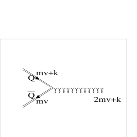
Figure 1: Heavy quark-antiquark pair annihilation into a gluon of momentum $2mv+k$. For simplicity the heavy quark and antiquark are assumed to carry momenta $mv+k$ and $mv$ respectively. Such process could be described meaningfully by HQET if $k$ is small w.r.t the heavy quark mass $m$, i.e. the relative velocity of both heavy quarks is small. The same statement is valid for heavy quark pair production near theshold.

Assuming the same conditions as in figure 1, we can write for almost free heavy quarks in the initial- or final-state

$$H_{v}^{(+)} = (iv{\cdot}\overrightarrow{\partial}+2m-i\epsilon)^{-1}i\overrightarrow{\partial{\!\!\!/}}_{\bot}h_{v}^{(+)}$$ (36)

$$H_{v}^{(-)} = (-iv{\cdot}\overrightarrow{\partial}+2m-i\epsilon)^{-1}i\overrightarrow{\partial{\!\!\!/}}_{\bot}h_{v}^{(-)}$$ (37)

and for the conjugate fields

$$\overline{H}_{v}^{(+)} = \overline{h}_{v}^{(+)}i\overleftarrow{\partial{\!\!\!/}}_{\bot}(iv{\cdot}\overleftarrow{\partial}-2m+i\epsilon)^{-1}$$ (38)

$$\overline{H}_{v}^{(-)} = \overline{h}_{v}^{(-)}i\overleftarrow{\partial{\!\!\!/}}_{\bot}(-iv{\cdot}\overleftarrow{\partial}-2m+i\epsilon)^{-1}$$ (39)

Neglecting the soft gluon interaction among heavy quarks amounts to describe them as plane waves, i.e. actually no bound states as a first approximation [13].

Expanding and retaining the first non-null terms in Eqs. (36) and (39) one easily gets

$$H_{v}^{(+)}\ =\ \frac{i\overrightarrow{\partial{\!\!\!/}}_{\bot}}{2m}\ h_{v}^{(+)}$$ (40)

$$\overline{H}_{v}^{(-)}\ =\ -\ \overline{h}_{v}^{(-)}\ \frac{i\overleftarrow{\partial{\!\!\!/}}_{\bot}}{2m}$$ (41)

In momentum space ($k$ representing the residual momentum of the heavy quark w.r.t. the heavy antiquark) one may write to the same order in the $1/m$ expansion

$$u\ =\ \biggl{(}1\ +\ \frac{k{\!\!\!/}_{\bot}}{2m}\biggr{)}\ u_{h}\ e^{-ik{\cdot}x}$$ (42)

where $u_{h}$ stands for the HQET spinor and $u$ for the full QCD spinor. On the other hand

$$\overline{v}\ =\ \overline{v}_{h}$$ (43)

where $v_{h}$ stands for the HQET anti-spinor for a heavy antiquark without residual momentum and $v$ denotes the full QCD anti-spinor.

Since $\overline{H}^{(-)}{\equiv}0$ in this case, Eq. (14) simplifies in this particular case to

$${\cal L}^{(-+)}=e^{-i2mv{\cdot}x}\ [\ \overline{h}_{v}^{(-)}i\overrightarrow{D{\!\!\!\!/}}_{\bot}h_{v}^{(+)}-\overline{h}_{v}^{(-)}(iv{\cdot}\overrightarrow{D}+2m)H_{v}^{(+)}\ ]$$ (44)

It is convenient to emphasize that the covariant derivative in the above expression contains the strong gluonic field while the $H_{v}^{(+)}$ field satisfies Eq. (36). Thus the effective annihilation vertex into a final gluon can be read off as

$$i{\Gamma}_{eff}^{\mu}\ =\ igT_{a}\ \biggl{[}\ {\gamma}^{\mu}\ -\ i\frac{{\sigma}^{\mu\nu}k_{\nu}}{2m}\ +\ \frac{k^{2}}{4m^{2}}{\gamma}^{\mu}\ +\ ...\ \biggr{]}$$ (45)

Indeed, from the terms of (14) coupling to one gluon we may write the effective vertex as

$$i{\Gamma}_{eff}^{\mu}\ =\ igT_{a}\ \biggl{[}\ {\gamma}^{\mu}\ -\ \frac{k{\!\!\!/}}{2m}v^{\mu}\ +\ ...\ \biggr{]}$$ (46)

and then using the relation (A.2) written as

$$P_{-}\ (v^{\mu}{\gamma}^{\nu})\ P_{+}\ =\ P_{-}\ (i{\sigma}^{\mu\nu}\ +\ {\gamma}^{\mu}v^{\nu})\ P_{+}$$ (47)

we obtain (45) if the on-shell condition for the heavy quark is fulfilled, i.e.

$$v{\cdot}k\ =\ -\frac{k^{2}}{2m}$$

In fact the same result could be directly derived from full (tree-level) QCD by making the appropriate transformations in the Feynman amplitude of the vertex itself, namely

$$igT_{a}\ \overline{v}\ {\gamma}^{\mu}\ u {\rightarrow} igT_{a}\ \overline{v}_{h}\ {\gamma}^{\mu}\biggl{[}\ 1\ +\ \frac{k{\!\!\!/}_{\bot}}{2m}\ +...\biggr{]}\ u_{h}$$ (48)

$$= igT_{a}\ \overline{v}_{h}\ {\gamma}^{\mu}\biggl{[}\ 1\ +\ \frac{k{\!\!\!/}}{2m}\ -\ \frac{(v{\cdot}k)}{2m}\ +\ ...\ \biggr{]}\ u_{h}$$

recovering the result expressed in Eq. (45) since

$$P_{-}\ \biggl{(}\frac{{\gamma}^{\mu}k{\!\!\!/}}{2m}\biggr{)}\ P_{+}\ =\ P_{-}\ \biggl{(}-i\frac{{\sigma}^{\mu\nu}k_{\nu}}{2m}\biggr{)}\ P_{+}$$

The above exercise shows that indeed the effective theory and full QCD lead to the same annihilation vertex at the same order in the $1/m$ expansion.

4 Summary and last remarks

We have derived a complete tree-level heavy-quark effective Lagrangian in terms of the effective fields $h_{v}^{(\pm)}$ keeping the particle-antiparticle mixed pieces allowing for heavy quark-antiquark pair annihilation/creation processes. Let us note that such pieces are not generally shown in similar developments in the literature.

Indeed, it may seem quite striking that a low-energy effective theory could be appropriate to deal with hard processes such as $Q\overline{Q}$ annihilation or creation. The keypoint is that assuming a kinematic regime where heavy quarks/antiquarks are almost on-shell and moving with small relative velocity, one can factor out the strong momentum dependence associated with the heavy quark mass both at the initial and final state (i.e. including also the strong gluonic field) so that a description based on the low frequency modes of the fields still makes sense. Such a kinematic regime is well matched by heavy quarkonium states and by colored intermediate bound states in the so-called color-octet model recently introduced [14] to account for high rates of heavy resonance hadroproduction at the Fermilab Tevatron [15].

However, a systematic inverse heavy-quark mass expansion of the mixed pieces $L^{(-+)}$ and $L^{(+-)}$ is not permitted if the classical equations of motion for heavy quarks in the background of a strong gluonic field are employed. This is because Eq. (35), where effective fields $H_{v}^{(\pm)}$ are written in terms of $h_{v}^{(\pm)}$, is not a convergent expression due to the momentum dependence of the strong gluonic field, of order of twice the heavy quark mass. (We might say in a loose way that the $H_{v}^{(\pm)}$ fields are not $``$small” anymore.) As a consequence the Lagrangian pieces $L^{(-+)}$ and $L^{(+-)}$ as expressed in Eqs. (28-29) or (33-34) are not expansible in powers of the reciprocal of the heavy quark mass. Moreover, let us note that in using such equations of motion heavy quarks would be assumed in the background of a strong color field. However, we are rather interested in a kinematic regime where initial- or final-state heavy quarks interact softly among themselves or with light constituents.

Therefore, if the classical equations of motion deriving from the $L^{(++)}$ and $L^{(--)}$ sectors are used to remove the unwanted degrees of freedom in the $L^{(-+)}$ and $L^{(+-)}$ sectors, then convergent and meaningful powers series are obtained. In particular, assuming an annihilation process with initial-state quarks (or final-state quarks for a creation process) satisfying the Dirac equation of motion for free fermions, the vertex Feynman rule is easily obtained, in accordance with full QCD vertex expanded to the same $1/m$ order.

In summary, we conclude that heavy quark-antiquark pair annihilation and creation can be meaningfully described starting from a tree-level HQET Lagrangian for special kinematic regimes of current interest in heavy flavor physics.

Acknowledgments

We thank V. Giménez, A. Pineda and J. Soto for reading the manuscript and critical comments.

Appendices

Appendix A Useful spinorology

In this appendix we gather some well-known simple formulas together with some others not so commonly found in the literature, exhaustively employed throughout this work

$$v{\!\!\!/}h_{v}^{(+)}=h_{v}^{(+)}\ ;\ v{\!\!\!/}H_{v}^{(+)}=-H_{v}^{(+)}\ ;\ v{\!\!\!/}h_{v}^{(-)}=-h_{v}^{(-)}\ ;\ v{\!\!\!/}H_{v}^{(-)}=H_{v}^{(-)}$$

Then, the projectors $P_{\pm}=(1{\pm}v{\!\!\!/})/2$ acting on the fields yield

$$P_{+}\ h_{v}^{(+)}=h_{v}^{(+)}\ \ ;\ \ P_{-}\ h_{v}^{(+)}=0\ \ ;\ \ P_{-}\ H_{v}^{(+)}=H_{v}^{(+)}\ \ ;\ \ P_{+}\ H_{v}^{(+)}=0$$

$$P_{-}\ h_{v}^{(-)}=h_{v}^{(-)}\ \ ;\ \ P_{+}\ h_{v}^{(-)}=0\ \ ;\ \ P_{+}\ H_{v}^{(-)}=H_{v}^{(-)}\ \ ;\ \ P_{-}\ H_{v}^{(-)}=0$$

and analogously for the conjugate fields $\overline{h}_{v}^{(+)}$, $\overline{h}_{v}^{(-)}$, $\overline{H}_{v}^{(+)}$ and $\overline{H}_{v}^{(-)}$. Therefore orthogonality implies

$$\overline{h}_{v}^{(-)}h_{v}^{(+)}\ =\ \overline{h}_{v}^{(-)}H_{v}^{(-)}\ =\ \overline{H}_{v}^{(-)}h_{v}^{(-)}\ =\ \overline{H}_{v}^{(-)}H_{v}^{(+)}\ =\ 0$$

but

$$\overline{h}_{v}^{(-)}H_{v}^{(+)}\ {\neq}\ 0\ \ ;\ \overline{h}_{v}^{(-)}{\gamma}^{\mu}\ h_{v}^{(+)}\ {\neq}\ 0$$

and so on.

In the particle-particle sector of the effective theory, it is also well-known that the vector current can be expressed as

$$\overline{h}_{v}^{(+)}\ {\gamma}^{\mu}\ h_{v}^{(+)}\ =\ \overline{h}_{v}^{(+)}\ v^{\mu}\ h_{v}^{(+)}$$

On the other hand, since

$$P_{-}\ {\gamma}^{\mu}{\gamma}^{\nu}\ P_{+}\ =\ P_{-}\ ({\gamma}^{\mu}v^{\nu}\ -\ v^{\mu}{\gamma}^{\nu})\ P_{+}$$ (A.1)

an equivalent relation in the particle-antiparticle sector reads

$$\overline{h}_{v}^{(-)}\ {\gamma}^{\mu}{\gamma}^{\nu}\ h_{v}^{(+)}\ =\ \overline{h}_{v}^{(-)}\ {\gamma}^{\mu}v^{\nu}\ h_{v}^{(+)}\ -\ \overline{h}_{v}^{(-)}\ v^{\mu}{\gamma}^{\nu}\ h_{v}^{(+)}$$

This implies that

$$P_{-}\ (-i\sigma^{\mu\nu})\ P_{+}\ =\ P_{-}\ ({\gamma}^{\mu}v^{\nu}-v^{\mu}{\gamma}^{\nu})\ P_{+}$$ (A.2)

and

$$P_{-}\ (-i\sigma^{\mu\nu})\ P_{+}\ =\ P_{-}\ ({\gamma}^{\mu}{\gamma}^{\nu})\ P_{+}$$ (A.3)

and thus

$$\overline{h}_{v}^{(-)}\ (-i\sigma^{\mu\nu})\ h_{v}^{(+)}\ =\ \overline{h}_{v}^{(-)}\ {\gamma}^{\mu}v^{\nu}\ h_{v}^{(+)}\ -\ \overline{h}_{v}^{(-)}\ v^{\mu}{\gamma}^{\nu}\ h_{v}^{(+)}$$ (A.4)

Hence

$$\overline{h}_{v}^{(-)}\ (-i\sigma^{\mu\nu}v_{\nu})\ h_{v}^{(+)}\ =\ \overline{h}_{v}^{(-)}\gamma^{\mu}\ h_{v}^{(+)}$$ (A.5)

In the particle-particle sector odd combinations of gamma matrices can be simplified by replacing some ${\gamma}$ matrices by $v$’s, whereas in the particle-antiparticle sector even combinations lead to the same kind of simplification. For example,

$$P_{+}\ {\gamma}^{\mu}{\gamma}^{\nu}{\gamma}^{\alpha}\ P_{+}\ =\ P_{+}\ (v^{\mu}{\gamma}^{\nu}{\gamma}^{\alpha}\ -\ {\gamma}^{\mu}v^{\nu}{\gamma}^{\alpha}\ +\ {\gamma}^{\mu}{\gamma}^{\nu}v^{\alpha})\ P_{+}$$ (A.6)

Permutation of the projectors $P_{\pm}$ in all above expressions implies the overall substitution $v{\rightarrow}-v$. Moreover, similar relations are satisfied if the $\gamma$ matrices are sandwiched between heavy quark spinors and/or anti-spinors obeying $v{\!\!\!/}u_{h}=u_{h}$ and $v{\!\!\!/}v_{h}=-v_{h}$.

References

• [1] B. Grinstein, Annu. Rev. Nucl. Part. Sci., 42 (1992) 101.
• [2] M. Neubert, Phys. Rep. 245 (1994) 259.
• [3] T. Mannel, W. Roberts and Z. Ryzak, Nucl. Phys. B368 (1992) 204.
• [4] N. Isgur and M.B. Wise, Phys. Lett. B232 (1989) 113; B237 (1990) 527.
• [5] M. Neubert, Int. J. Mod. Phys. A11 (1996) 4173.
• [6] A. Pich, FTUV/98-46, hep-ph/9806303.
• [7] M.A. Sanchis-Lozano, Nuov. Cim. A110 (1997) 295.
• [8] Y.L. Wu, Mod. Phys. Lett. A8 (1993) 819.
• [9] U. Aglietti and S. Capitani, Nucl. Phys. B432 (1994) 315.
• [10] T. Mannel and G. Schuler, Z. Phys. C67 (1995) 159.
• [11] S. Balk, J.G. Körner, D. Pirjol, Nucl. Phys. B428 (1994) 499.
• [12] H. Georgi, Phys. Lett. B240 (1990) 447.
• [13] F. Hussain, J.G. Körner and G. Thompson, Ann. Phys. 206 (1991) 334.
• [14] E. Braaten and S. Fleming, Phys. Rev. Lett. 74 (1995) 3327.
• [15] CDF Collaboration, F. Abe et al., Phys. Rev. Lett. 69 (1992) 3704.