FTUV/98-67

IFIC/98-68

Generalized Hypergeometric Functions and the Evaluation of Scalar One-loop Integrals in Feynman Diagrams

Luis G. Cabral-Rosetti and Miguel A. Sanchis-Lozano

Departamento de Física Teórica and IFIC
Centro Mixto Universidad de Valencia-CSIC
46100 Burjassot, Valencia (Spain)

Present and future high-precision tests of the Standard Model and beyond for the fundamental constituents and interactions in Nature are demanding complex perturbative calculations involving multi-leg and multi-loop Feynman diagrams. Currently, large effort is devoted to the search for closed expressions of loop integrals, written whenever possible in terms of known - often hypergeometric-type - functions. In this work, the scalar three-point function is re-evaluated by means of generalized hypergeometric functions of two variables. Finally, use is made of the connection between such Appell functions and dilogarithms coming from a previous investigation, to recover well-known results.

Keywords: Feynman diagrams; loop integrals; hypergeometric series, Appell function; dilogarithm

1. Introduction

Present and foreseen unprecedented high-precision experimental results from $e^{+}e^{-}$ colliders (LEP, B Factories), hadron-hadron colliders (Tevatron, LHC) and electron-proton colliders (HERA) are demanding refined calculations from the theoretical side as stringent tests of the Standard Model for the fundamental constituents and interactions in Nature. Moreover, possible extensions beyond the Standard Model (e.g. Supersymmetry) often require high-order calculations where such new effects eventually would manifest.

In fact, much effort has been devoted so far to develop systematic approaches to the evaluation of complicated Feynman diagrams, looking for algorithms (see for example [10, 4] and references therein), or recurrence algorithms [13, 22, 21], to be implemented in computer program packages to cope with the complexity of the calculation. On the other hand, the fact that such algorithms could be based, at least in part, on already defined functions represents a great advantage in many respects, as for example the knowledge of their analytic properties (e.g. branching points and cuts with physical significance), reduction to simpler cases with the subsequent capability of cross-checks and so on. Commonly-used representations for loop integrals involve special functions like polylogarithms, generalized Clausen’s functions, etc.

Furthermore, over this decade the role of generalized hypergeometric functions in several variables to express the result of multi-leg and multi-loop integrals arising in Feynman diagrams has been widely recognized [5, 6, 7, 8, 3, 2]. The special interest in using hypergeometric-type functions is twofold:

• Hypergeometric series are convergent within certain domains of their arguments, physically related to some kinematic regions. This affords numerical calculations, in particular implementations as algorithms in computer programs. Moreover, analytic continuation allows to express hypergeometric series as functions outside those convergence domains.

• The possibility of describing final results by means of known functions instead of ad hoc power series is interesting by itself. This is especially significant for hypergeometric functions because of their deep connection with special functions whose properties are well established in the mathematical literature.

In this paper we mainly focus on the second point, although our aim is much more modest than searching for any master formula or method regarding complex Feynman diagrams. Rather we re-examine the scalar three-point function for massive external and internal lines, already solved in terms of dilogarithms [14]. The novelty of this work consists of solving and expressing the three-point function $C_{0}$, in terms of a set of Appell functions whose arguments are combinations of kinematic quantities. Then, by using a theorem already proved in an earlier publication [16], we end up with sixteen dilogarithms, recovering a well-known result [14]. The elegant relationship shown in [16] between Gauss and dilogarithmic functions might be a hint to look for more general connections that, hopefully, could be helpful for finding compact expressions or algorithms in Feynman calculations.

2. A simple relation between generalized hypergeometric series and dilogarithms

There are four independent kinds of Appel functions [19], named $F_{1},\ F_{2},\ F_{3},\ F_{4}$. In particular, the $F_{3}$ series is defined as

$$F_{3}[a,a^{\prime},b,b^{\prime};c;x,y]\ =\ \sum_{m=0}^{\infty}\sum_{n=0}^{\infty}\frac{(a)_{m}(a^{\prime})_{n}(b)_{m}(b^{\prime})_{n}}{(c)_{m+n}}\frac{x^{m}}{m!}\frac{y^{n}}{n!}$$ (1)

which exists for all real or complex values of $a,\ a^{\prime},\ b,\ b^{\prime}$ and $c$ except $c$ a negative integer. With regard to its convergence, the $F_{3}$ series is (absolutely) convergent when both ${\mid}x{\mid}<1$ and ${\mid}y{\mid}<1$; $(a)_{m}={\Gamma}(a+m)/{\Gamma}(a)$ stands for the Pochhammer symbol.

Below we re-write our main theorem published in [16] showing a simple connection between dilogarithms [12] and a particular $F_{3}$ Appell function:

$$\frac{1}{2}xy\ F_{3}[1,1,1,1;3;x,y]=Li_{2}(x)+Li_{2}(y)-Li_{2}(x+y-xy)$$ (2)

${\mid}\arg{(1-x)}{\mid}<\pi$, ${\mid}\arg{(1-y)}{\mid}<\pi$ and ${\mid}\arg{(1-x)(1-y)}{\mid}<\pi$.

Note that the validity of the theorem can be extended dropping the restriction ${\mid}\arg{(1-x)(1-y)}{\mid}<\pi$ by slightly modifying Eq. (2):

$$\frac{1}{2}xy\ F_{3}[1,1,1,1;3;x,y]=Li_{2}(x)+Li_{2}(y)-Li_{2}(x+y-xy)-{\eta}(1-x,1-y)\ln{(x+y-xy)}$$

where ${\mid}\arg{(1-x)}{\mid}<\pi$, ${\mid}\arg{(1-y)}{\mid}<\pi$ and ${\eta}(a,b)=\ln{(ab)}-\ln{a}-\ln{b}$. The principal branches of the logarithm and dilogarithm are understood.

As an illustrative particular case one finds

$$x\ F_{3}[1,1,1,1;3;x,y=1]\ =\ 2x\ _{3}F_{2}(1,1,1;2,2;x)\ =\ 2\ Li_{2}(x)$$ (3)

Other related expressions derived from Eq. (2) may be found in [16] . Moreover, an extension of relation (3) to polylogarithms [12] can be easily checked

$$x\ F_{1:q-2;0}^{0:q;2}[\{1\}_{q},\{1\}_{2};\{2\}_{q-2};3;x,y=1]\ =\ 2x\ _{q+1}F_{q}[\{1\}_{q+1};\{2\}_{q};x]\ =\ 2\ Li_{q}(x)$$ (4)

where $F_{1:q-2;0}^{0:q;2}$ stands for a kind of Kampé de Fériet function [1] (or generalized Lauricella function of two variables [20, 9]) defined as a series as:

$$F_{1:t;0}^{0:r;s}[\{b\}_{r},\{b^{\prime}\}_{s};\{d\}_{t};c;x,y]\ =\ \sum_{m=0}^{\infty}\sum_{n=0}^{\infty}\frac{(b_{1})_{m}...(b_{r})_{m}(b^{\prime}_{1})_{n}...(b^{\prime}_{s})_{n}}{(d_{1})_{m}...(d_{t})_{m}\ (c)_{m+n}}\ \frac{x^{m}}{m!}\frac{y^{n}}{n!}$$

Proof. It follows easily by writing the equality

$$F_{1:q-2;0}^{0:q;2}[\{1\}_{q},\{1\}_{2};\{2\}_{q-2};3;x,y=1]\ =\ \sum_{m=o}^{\infty}\frac{\{1\}_{q}}{\{2\}_{q-2}(3)_{m}}\ \frac{x^{m}}{m!}\ _{2}F_{1}(1,1;3+m;1)$$

and using the Gauss summation relation in the latter ${}_{2}F_{1}$ series.

3. Application to the evaluation of One-Loop Integrals

In this Section, we present a simple but important application of the connection (2) between hypergeometric series and dilogarithms to the evaluation of scalar integrals appearing at one-loop level in Feynman diagrams.

In particular we shall write the scalar three-point function corresponding to the diagram of Figure 1:

Figure 1: Notation used for external and internal momenta and masses

$$C_{0}(p_{1}^{2},p_{2}^{2},p_{3}^{2};m_{1}^{2},m_{2}^{2},m_{3}^{2})=\int\ d^{4}q\ \frac{1}{[q^{2}-m_{2}^{2}][(q+p_{1})^{2}-m_{3}^{2}][(q+p_{1}+p_{2})^{2}-m_{1}^{2}]}$$ (5)

After Feynman parameterization [23] one arrives at the following double integral

$$C_{0}(p_{1}^{2},p_{2}^{2},p_{3}^{2};m_{1}^{2},m_{2}^{2},m_{3}^{2})/i{\pi}^{2}\ =\ \ \int_{0}^{1}u\ du\ \int_{0}^{1}dv\ \frac{1}{Q^{2}}$$ (6)

where

$$Q^{2}=u(1-u)(1-v)p_{1}^{2}+u^{2}v(1-v)p_{2}^{2}+u(1-u)vp_{3}^{2}-uvm_{1}^{2}-(1-u)m_{2}^{2}-u(1-v)m_{3}^{2}$$ (7)

Let us remark that in performing the first parametric integral in Eq. (6), either an external or an internal mass should vanish in order to get a hypergeometric function of the type ${}_{2}F_{1}(1,1;2;z)$ (with $z$ as a combination of masses and Feynman parameters). Specifically, one should drop either the $p_{2}^{2}$-term in the denominator $Q^{2}$ (in this case firstly integrating over $v$) or the $m_{2}^{2}$-term (in this case firstly integrating over $u$), of course the particular choice of index 2 by no means representing any loss of generality.

Hence, the basic idea is to follow a procedure to get rid of any of those masses, so that one can express the final result in terms of generalized Gauss functions in two variables, after performing the parametric integrations over $v$ and $u$ consecutively [17]. In fact, this goal can be achieved in a standard way by means of a $``$trick” introduced by Passarino and Veltman [15] in this context, using a propagator identity and defining a set of unphysical vectors [23, 17]. Then, the loop integral (5) can be splitted into two pieces corresponding to the sum of two three-point functions with either an internal or an external mass equal to zero. The latter possibility may be exploited for one (at least) timelike external momentum - in fact this is generally the case at next-to-leading order calculations since for any real scattering or decay process there is always an external timelike or lightlike momentum.

Therefore, under the assumption of any timelike external momentum we write below the final expression of the three-point function for massive internal and external lines in a very closed form:

$$C_{0}(p_{1}^{2},p_{2}^{2},p_{3}^{2};m_{1}^{2},m_{2}^{2},m_{3}^{2})/i{\pi}^{2} = \frac{{\sigma}_{\alpha}}{2\lambda^{1/2}(p_{1}^{2},p_{2}^{2},p_{3}^{2})}\ {\times}$$

$$\sum_{i=1}^{2}\ \biggl{(}\ [\ R(x_{i},y)-R(x_{i}^{\prime},y)\ ]\ -\ [\ \alpha{\leftrightarrow}(1-\alpha),1{\leftrightarrow}3\ ]\ \biggr{)}$$

where the interchange of indices $1{\leftrightarrow}3$ does not apply inside $\alpha$. The notation is the following:

• Each term of the summation (we use the same symbol $R$ as in [14]) can be written in terms of an Appell’s function according to

  $$R(x_{i},y)\ =\ \frac{1}{2}\ x_{i}y\ F_{3}[1,1,1,1;3;x_{i},y]$$

• ${\alpha}$ is given by any of the two solutions:

  $${\alpha}_{\pm}\ =\ \frac{p_{1}^{2}+p_{2}^{2}-p_{3}^{2}\ {\pm}\ {\lambda}^{1/2}(p_{1}^{2},p_{2}^{2},p_{3}^{2})}{2p_{2}^{2}}$$

  with ${\lambda}$ standing for the Källen function, $\lambda(x,y,z)=(x-y-z)^{2}-4yz$; ${\sigma}_{\alpha}={\mp}1$ according to the choice for the square root of ${\alpha}_{\pm}$.

  It is not difficult to verify the independence of the result as expressed in Eq. (8) on the choice of the sign for $\alpha$ using the initial symmetry of the scalar integral under the permutation of indices, in particular $1{\leftrightarrow}3$ (now including $\alpha$ under such index permutation). Hence the first four $R$ terms in (8) would depend on $\alpha(3,1)$, instead of $\alpha(1,3)$. Since $\alpha_{+}(3,1)=1-\alpha_{-}(1,3)$) one arrives quickly to the above-mentioned conclusion taking into account $\sigma_{\alpha}$.

• Variables $x_{i}$ and $x_{i}^{\prime}$ is defined as: $x_{i}=1/r_{i}$ and $x_{i}^{\prime}={\alpha}/t_{i}$ where

  $$r_{1,2}\ =\ \frac{p_{1}^{2}+m_{3}^{2}-m_{2}^{2}\ {\pm}\ {\lambda}^{1/2}(p_{1}^{2},m_{3}^{2},m_{2}^{2})}{2p_{1}^{2}}$$

  and

  $$t_{1,2}\ =\ \frac{p_{2}^{2}+m_{3}^{2}-m_{1}^{2}\ {\pm}\ {\lambda}^{1/2}(p_{2}^{2},m_{3}^{2},m_{1}^{2})}{2p_{2}^{2}}$$

• The $y$ variable is given by

  $$y\ =\ \frac{\alpha\ {\lambda}^{1/2}(p_{1}^{2},p_{2}^{2},p_{3}^{2})}{(1-\alpha)[-p_{1}^{2}+m_{3}^{2}-m_{2}^{2}]+\alpha[-p_{3}^{2}+m_{1}^{2}-m_{2}^{2}]}$$

Now, using Eq. (2) the scalar one-loop integral of Figure 1 can be directly expressed in terms of sixteen dilogarithms since there is a pairwise cancellation between eight $Li_{2}(y)$ functions, leading to a similar result as obtained in Ref. [14]. Therefore, it becomes apparent the usefulness of the connection between dilogarithms and generalized hypergeometric functions shown in this theorem [16]. Expectedly, further relations involving multiple hypergeometric functions and polylogarithms or related functions [11] could be discovered [18], with the possibility of application to more complicated loop integrals.

Finally, for the sake of completeness we show in Figure 2 some (finite) results considering several special values for the internal and external masses, as limits deriving from the main expression (8).

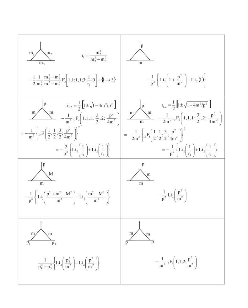
Figure 2: Special finite cases for the $C_{0}/i{\pi}^{2}$ three-point function. Missing symbols on external and internal lines mean zero mass.

4. Summary and last remarks

In this paper, we have shown that the familiar scalar three-point function $C_{0}$ arising in Feynman diagram calculations, can be expressed in terms of eight Appell functions whose arguments are simple combinations of internal and external masses. The extension to complex values of the masses (of concern in several interesting physical cases) can be performed via analytic continuation of the hypergeometric functions. Moreover, by invoking a theorem proved in [16] connecting dilogarithms and generalized hypergeometric functions, we have recovered a well-known formula for the evaluation of $C_{0}$ [14]. Finally, let us stress that, although its simplicity, this work is on the line of searching for closed expressions of Feynman loop integrals. On the other hand but in a complementary way, such physical requirements should motivate, on the mathematical side, further developments of the still largely unknown field on multiple hypergeometric functions (as compared to one-variable hypergeometric functions) and their connections to generalized polylogarithms [11].

Acknowledgments

This work has been partially supported by CICYT under grant AEN-96/1718. M.A.S.L. acknowledges an Acción Especial (code 6223080) by the regional government Generalitat Valenciana. L.G.C.R. has been supported by a fellowship from the D.G.A.P.A.-U.N.A.M. (México).

References

- [1] P. Appell and J. Kampé de Fériet, Fonctions Hypergéometriques et Hyperesphériques. Polynomes d’Hermite, Gautiers-Villars, Paris (1926).
- [2] S. Bauberger, F.A. Berends, M. Böhm, M. Buza, Analytical and numerical methods for massive two-loop self-energy diagrams, Nucl. Phys. B 434 (1995) 383-407.
- [3] F.A. Berends, M. Böhm, M. Buza, R. Scharf, Closed expressions for specific massive multiloop self-energy diagrams, Z. Phys. C 63 (1994) 227-234.
- [4] L. Brücher, J. Franzkowski, D. Kreimer, A Program package calculating one-loop integrals, Comput. Phys. Commun. 107 (1997) 281-292.
- [5] A.I. Davydychev, Some exact results for N-point massive Feynman integrals, J. Math. Phys. 32 (1991) 1052-1058.
- [6] A.I. Davydychev, General results for massive N-point Feynman diagrams with different masses, J. Math. Phys. 33 (1992) 258-369.
- [7] A.I. Davydychev, Recursive algorithm for evaluating vertex-type Feynman integrals, J. Phys. A 25 (1992) 5587-5596.
- [8] A.I. Davydychev, Standard and hypergeometric representations for loop diagrams and the photon-photon scattering, hep-ph/9307323.
- [9] H. Exton, Handbook of Hypergeometric Integrals, Ellis-Horwood, Chicester UK, 1978.
- [10] T. Hahn and M. Pérez-Victoria, Automatized one-loop calculations in four and D dimensions, UG-FT-87/98, hep-ph/9807565.
- [11] K.S. Kölbig, Nielsen’s generalized polylogarithms, SIAM J. Math. Anal. A7 (1987) 1232-1258.
- [12] L. Lewin, Polylogarithms and Associated Functions, North-Holland, New York 1981.
- [13] R. Mertig, R. Scharf, TARCER - A Mathematica program for the reduction of two-loop propagator integrals, hep-ph/9801383.
- [14] G.J. van Oldenborgh and J.A.M. Vermaseren, New algorithms for one-loop integrals, Z. Phys. C 46 (1990) 425-437.
- [15] G. Passarino and M. Veltman, One-Loop corrections for annihilation into in the Weinberg model, Nucl. Phys. B 160 (1979) 151-161.
- [16] M.A. Sanchis-Lozano, Simple connections between generalized hypergeometric series and dilogarithms, J. Comput. Appl. Math. 85 (1997) 325-331.
- [17] M.A. Sanchis-Lozano, A Calculation of Scalar one-loop Integrals by means of generalized hypergeometric functions, IFIC/91-49.
- [18] M.A. Sanchis-Lozano, in preparation.
- [19] L.C. Joan Slater, Generalized Hypergeometric Functions, Cambridge University Press (1966).
- [20] H.M. Srivastava, M.C. Daoust, Nederl. Akad. Wetensch. Proc. A 72 (1969) 449-459.
- [21] O.V. Tarasov, A new approach to the momentum expansion of multiloop Feynman diagrams, Nucl. Phys. B 480 (1996) 397-412.
- [22] O.V. Tarasov, Generalized recurrence relations for two-loop propagator integrals with arbitrary mases, Nucl. Phys. B 502 (1997) 455.
- [23] G. ’t Hooft and M. Veltman, Scalar one-loop integrals, Nucl.Phys. B 153 (1979) 365-401.