ANALYTIC QCD FLAVOR THRESHOLDS THROUGH TWO LOOPS

In this talk , we present a recently suggested way on how to analytically incorporate massive threshold effects into observables calculated in massless QCD. No matching is required since the renormalization scale is in this approach connected to the physical momentum transfer between static quarks in a color singlet state. We discuss massive fermionic corrections to the heavy quark potential through two loops. The calculation uses a mixed approach of analytical, computer-algebraic and numerical tools including Monte Carlo integration of finite terms. Strong consistency checks are performed by ensuring the proper cancellation of all non-local divergences by the appropriate counterterms and by comparing with the massless limit. The size of the effect for the (gauge invariant) fermionic part of $\alpha_{V}({\bf q^{2}},m^{2})$ relative to the massless case at the charm and bottom flavor thresholds is found to be of order $33\%$.

1 Introduction

1.1 Analytic Thresholds at one Loop

In the $MS$ and $\overline{MS}$ renormalization schemes, the running of the QCD coupling $\alpha_{s}$, by construction, does not “know” about the masses, $m_{q}$, of quarks. The $\beta$ function $\!{}^{{\bf?},{\bf?}}$ describes the evolution of the strong coupling “constant” in the asymptotic regime, i.e. for values of the renormalization scale $\mu\gg m_{q}$. Near the quark flavor thresholds one has to turn to effective descriptions which match threories with $n$ massless quarks onto a theory with $n-1$ massless and one massive flavor at the “heavy” quark threshold. In this way the dependence on the dimensional regularization mass parameter $\mu$ is reduced to next to leading order effects by giving up the analyticity of the coupling at the flavor threshold $\!{}^{{\bf?},{\bf?},{\bf?}}$.

While this procedure of matching conditions and effective descriptions is certainly workable, from a theoretical standpoint it would be advantageous to have a physical coupling constant definition which is analytic at thresholds. In addition, as a physical observable, the total derivative with respect to the renormalization scale $\mu$ vanishes. Such a system is given by identifying the ground state energy of the vacuum expectation value of the Wilson loop as the potential $V$ between a static quark-antiquark pair in a color singlet state $\!{}^{{\bf?},{\bf?},{\bf?},{\bf?},{\bf?},{\bf?}}$:

$$V(r,m^{2}_{q})=-\lim_{t\rightarrow\infty}\frac{1}{it}log\langle 0|Tr\;\{P\;exp\left(\oint dx_{\mu}A^{\mu}_{a}T^{a}\right)\}|0\rangle$$ (1)

where $r$ denotes the relative distance between the heavy quarks, $m_{q}$ the mass of “light” quarks contributing through loop effects and $T^{a}$ the generators of the gauge group. It is then convenient to define the effective charge $\alpha_{V}({\bf q}^{2},m^{2})$ as

$$V({\bf q}^{2},m_{q}^{2})\equiv-\frac{4\pi C_{F}\alpha_{V}({\bf q}^{2},m_{q}^{2})}{{\bf q}^{2}}$$ (2)

in momentum space with ${\bf q}^{2}\equiv q_{0}^{2}-q^{2}=-q^{2}>0$. The factor $C_{F}$ is the value of the Casimir operator $T^{a}T^{a}$ in the fundamental representation of the external sources and factors out to all orders in perturbation theory. As one is free to choose the representation of the external particles, we obtain the static gluino potential by adopting the adjoint representation.

Recently $\!{}^{{\bf?}}$, the effect of the massive fermionic one loop contributions to the heavy quark potential were incorporated into a continuous and smooth function $n_{f}\left(\rho_{q}\right)$ given to lowest order by

$$n^{o}_{f,V}\left(\rho_{q}\right) \equiv \frac{3\pi}{\alpha_{V}^{2}}\frac{\partial\alpha_{V}^{f_{1loop}}}{\partial Q}$$ (3)

$$= 1-\frac{6}{\rho_{q}}+\frac{24}{\rho^{\frac{3}{2}}_{q}\sqrt{4+\rho_{q}}}\tanh^{-1}\sqrt{\frac{\rho_{q}}{\rho_{q}+4}}$$

where $\rho_{q}\equiv\frac{Q^{2}}{m_{q}^{2}}$ and $Q^{2}\equiv-q^{2}$. The mass dependence of the physical $V$-scheme can now be transferred to the $\overline{MS}$ scheme by using the commensurate scale relation $\!{}^{{\bf?}}$ between the two schemes. Employing the multi scale approach of Ref. $\!{}^{{\bf?}}$ gives the following scale fixed relation through two loops $\!{}^{{\bf?}}$:

$$\alpha_{\overline{MS}}(Q)=\alpha_{V}(Q^{*})+2\frac{\alpha^{2}_{V}(Q^{**})}{\pi}+4.625\frac{\alpha^{3}_{V}(Q^{**})}{\pi^{2}}$$ (4)

with

$$Q^{*}=2.3Q\;\;,\;\;Q^{**}=6.539Q$$ (5)

whereas $Q^{***}$ to this order is not constrained. A first approximation is obtained, however, by setting $Q^{***}=Q^{**}$ $\!{}^{{\bf?}}$. Note that the scale $Q$ at one loop is a factor $0.4$ smaller than the physical scale $Q^{*}$.

1.2 Analytic ${\tilde{\alpha}}_{\overline{MS}}$

One is now free to adopt the commensurate scale relation of Eq. 4 as a definition of the extended scheme ${\tilde{\alpha}}_{\overline{MS}}$ $\!{}^{{\bf?}}$. At one loop we have therefore

$${\tilde{\alpha}}_{\overline{MS}}(Q)\equiv\alpha_{V}(Q^{*})+2\frac{\alpha^{2}_{V}(Q^{**})}{\pi}$$ (6)

for all scales $Q$. Eq. 6 not only provides an analytic extension of $MS$ like renormalized schemes, but it also ties down the renormalization scale $\mu$ to the physical scale with massive quarks, entering into the vacuum polarization contributions to $\alpha_{V}$. There is thus no scale ambiguity in perturbative expansions in $\alpha_{V}$ or ${\tilde{\alpha}}_{\overline{MS}}$. To lowest order we obtain in addition

$${\tilde{n}}^{o}_{f,{\overline{MS}}}\left(\frac{Q^{2}}{m_{q}^{2}}\right)=n^{o}_{f,V}\left(\frac{{Q^{*}}^{2}}{m_{q}^{2}}\right)$$ (7)

A very good ($\approx 1\%$) approximation is given by the following simple result for the one loop effective function of flavors:

$${\tilde{n}}^{o}_{f,{\overline{MS}}}\left(\frac{Q^{2}}{m_{q}^{2}}\right)\approx\frac{1}{1+\frac{5}{\rho_{q}}}$$ (8)

Figure 1: The sum over massive quark flavors for the effective analytic function ${\tilde{n}}^{o}_{f,{\overline{MS}}}\left(\frac{Q^{2}}{m_{q}^{2}}\right)$ given in Eq. 8.

Fig. 1 contains the analytic function $n_{f}$ summed over all quark flavors in comparison with the conventional step-function approach, which treats quarks as infinitely heavy below threshold and massless above.

1.3 Applications

It is of course possible to treat mass effects exactly within the $\overline{MS}$ scheme $\!{}^{{\bf?},{\bf?}}$ by explicitly calculating higher twist QCD corrections. In order to have a meaningful comparison between the different approaches of incorporating mass effects, we choose to compare the above treatment to the explicit corrections to an observable, here the quark part of the non-singlet hadronic width of the Z-boson, $\Gamma^{NS}_{had,q}$. Writing the QCD corrections in terms of an effective charge we have:

$$\Gamma_{had,q}^{NS}=\frac{G_{F}M_{Z}^{3}}{2\pi\sqrt{2}}\sum_{q}\{(g_{V}^{q})^{2}+(g_{A}^{q})^{2}\}\left[1+\frac{3}{4}C_{F}\frac{\alpha_{\Gamma,q}^{NS}(s)}{\pi}\right]$$ (9)

where the effective charge $\alpha_{\Gamma,q}^{NS}(s)$ contains all perturbative QCD corrections. At the one loop level we are left with a very simple expression

$$\frac{\alpha_{\Gamma,q}^{NS}(s)}{\pi} = \frac{{\tilde{\alpha}}_{\overline{MS}}(Q^{*})}{\pi}.$$ (10)

Figure 2: The relative difference between the calculation of $\alpha_{\Gamma,q}^{NS}(s)$ in the analytic extension of the $\overline{MS}$ scheme and the standard treatment of masses in the $\overline{MS}$ scheme. The discontinuities are due to the mismatch between the $s/m^{2}$ and $m^{2}/s$ expansions of the explicit QCD corrections in Refs. $\!{}^{{\bf?},{\bf?}}$.

This simple expression reflects the fact that the effects of quarks in the perturbative coefficients, both massless and massive, should be absorbed into the running of the coupling. The BLM-scale $\!{}^{{\bf?}}$ is $Q^{*}=0.7076\sqrt{s}$ for this observable $\!{}^{{\bf?}}$. The explicit higher twist corrections were calculated in Ref. $\!{}^{{\bf?},{\bf?}}$ as expansions in $\frac{m_{q}^{2}}{s}$ and $\frac{s}{m_{q}^{2}}$. Fig. 2 contains relative difference between the two approaches and can be seen to be in about permille agreement for perturbative values of the energy.

This remarkable level of agreement implies that in order to incorporate one loop massive QCD-flavor threshold effects into observables which are known only in massless QCD in the $\overline{MS}$ scheme, one just has to apply the analogous steps as above, namely replacing

$$n_{f}\longrightarrow{\tilde{n}}^{o}_{f,{\overline{MS}}}\left(\frac{Q^{2}}{m_{q}^{2}}\right)=n^{o}_{f,V}\left(\frac{{Q^{*}}^{2}}{m_{q}^{2}}\right)$$ (11)

where $Q^{*}$ is the BLM-scale of that process. In order to include all flavors one simply has the sum over all $m_{q}$ contributions as indicated in Fig. 1.

2 Two Loop Results

At the two loop level the situation becomes much more cumbersome. The massless case including pure gluonic corrections was calculated in Ref. $\!{}^{{\bf?}}$. Recently, the massive two loop corrections, depicted in Fig. 3, were obtained in Ref. $\!{}^{{\bf?}}$.

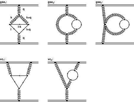
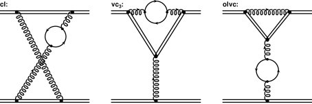
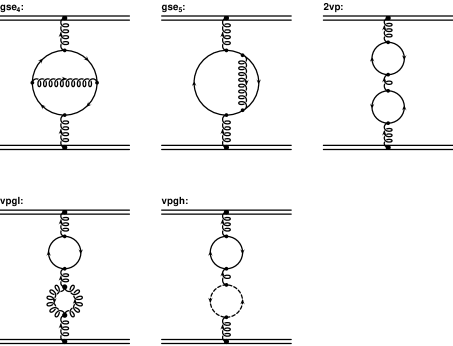
Figure 3: The two loop massive fermionic corrections to the heavy quark potential. The first two rows contain diagrams with a typical non-Abelian topology. Double lines denote the heavy quarks, single lines the “light” quarks. Color and Lorentz indices are suppressed in the first graph. The notation for the remaining digrams is analogous. The middle line includes the infra-red divergent “Abelian” Feynman diagrams. While the topology of these three diagrams is the same as in QED, they contribute to the potential only in the non-Abelian theory due to color factors  $C_{F}C_{A}$. In addition, although each diagram is infra-red divergent, their sum is infra-red finite. The infra-red finite Feynman diagrams with an Abelian topology are shown in the last two rows plus diagrams consisting of one loop insertions with non-Abelian terms.

The double lines denote the static color sources for which one employs the heavy quark effective Feynman rules (HQET), see for example Refs. $\!{}^{{\bf?}}$, while the rest contains the full QCD dynamics including massive fermion lines. The results in Ref. $\!{}^{{\bf?}}$ were obtained in the $MS$ renormalization scheme, related to the $\overline{MS}$ scheme through a simple scale shift

$$\mu_{{}_{MS}}=\sqrt{\frac{e^{\gamma}}{4\pi}}\mu_{{}_{\overline{MS}}}\;\;,$$ (12)

by a combined analytical and numerical approach. For the two point functions a tensor decomposition was performed following the techniques given in Ref. $\!{}^{{\bf?}}$. The algebraic manipulation language FORM $\!{}^{{\bf?}}$ was used for this purpose. The resulting scalar integrals are then solved by calculating the pole terms analytically and integrating over the remaining Feynman parameters numerically.

For the higher point functions this approach is no longer applicable due to the presence of the heavy quark propagators. It was found to be advantageous to integrate out the fermion loop analytically and then proceed with the remaining integrations. Details are given in Ref. $\!{}^{{\bf?}}$.

The required expansions in powers of $\epsilon=4-n$ were performed by MAPLE as was the translation of finite parts into FORTRAN. This latter point is crucial in face of the enormous complexity of the obtained results.

Strong consistency checks were performed including the explicit calculation of all $MS$ counterterms, shown in Fig. 4, to ensure the locality of renormalization constants, the correct gluon wave function renormalization constant and agreement with the $\frac{1}{\epsilon^{2}}$, $\frac{1}{\epsilon}$ pole terms from the massless calculation for the remaining three and four point two loop functions.

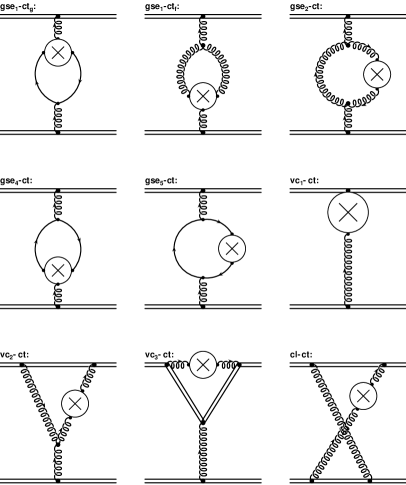
Figure 4: The counterterms corresponding to the massive two loop diagrams of Fig. 3.

Figure 5: The sum of the $\lambda^{2}$-dependent amplitudes and counterterms ${\cal M}^{k_{0}}_{cl}+{\cal M}^{k_{0}}_{vc_{3}}+{\cal M}_{olvc}+{\cal M}^{k_{0}}_{cl_{ct}}+{\cal M}^{k_{0}}_{{vc_{3}}_{ct}}$. Circles correspond to a choice of $q^{2}=-10GeV^{2}$ and $m=m_{c}$, triangles to $q^{2}=-100GeV^{2}$ and $m=m_{c}$ while the lower curve (squares) has $q^{2}=-100GeV^{2}$ and $m=m_{b}$. the overall normalization neglects color factors and the coupling strength. All data are obtained by using $10^{6}$ evaluations per iteration with VEGAS and 100 iterations. The statistical error is indicated and smaller than the symbols where invisible. The sum for each of the displayed sets of parameters is clearly independent of the IR-gluon mass regulator $\lambda$ as expected.

Furthermore, the absence of infrared divergences in the sum of the $MS$ renormalized diagrams ${\cal M}_{cl}$, ${\cal M}_{{vc}_{3}}$ and ${\cal M}_{olvc}$, which all contain infrared poles individually, is demonstrated in Fig. 5. $\frac{i}{k_{0}}$ denotes the heavy quark propagator and only terms with a dependence on $k_{0}$ needed to be regulated with a gluon mass. The results clearly demonstrate the infrared finiteness of the sum which contributes to the physical potential in Eq. 1.

The reason why these three amplitudes with an Abelian topology do contribute to the QCD potential but are absent in QED is connected to the exponentiation that is implicit in Eq. 1. The terms proportional to $C_{F}^{2}$ are actually already included in the potential by the exponentiation of the lower order Born and vacuum polarization contributions. In the non-Abelian theory, however, there is also a contribution proportional to $C_{F}C_{A}$, which cannot be obtained by the lower order terms and thus must be taken into account for the static QCD potential.

We also found perfect agreement for the numerical results for the finite, $MS$ renormalized expressions in the limit $m_{q}\longrightarrow 0$. The finite expressions were calculated with the Monte Carlo integrator VEGAS $\!{}^{{\bf?}}$ and Fig. 6 displays the weighted sum of all two loop $MS$ renormalized massive fermionic corrections to $\alpha_{V}$.

Figure 6: The complete two loop mass dependence of $\tilde{\alpha_{V}}\equiv\frac{\alpha^{f_{2\,loop}}_{V}}{g^{6}}$ for $m^{2}=m_{c}^{2}=(1.5GeV)^{2}$ (triangles) and $m^{2}=m_{b}^{2}=(4.5GeV)^{2}$ (open circles). The massless case is also included (line). In all three curves we use $\mu=0.031$. The deviation from the massless case at the flavor thresholds is of order of $33\%$ and is dominated by the new non-Abelian contributions

It was found that the overall curve is dominated by the non-Abelian threshold behavior (partially due to the extra factor of $C_{A}$). The “$m_{c}$-graph” (triangles) matches the massless case for lower values of $-q^{2}$ as $m_{c}^{2}\ll m_{b}^{2}$. At the respective thresholds we find roughly a 33 % deviation relative to the massless case. This could be very significant for applications where quark masses are expected to play an important part. At high values of $-q^{2}$ the theory becomes massless and reproduces the leading logarithmic terms obtained by the $\beta$-function analysis as these coefficients are scheme independent through two loops in a massless theory. These analyses can also be helpful for the incorporation of massive fermions in lattice analyses as the heavy quark potential is defined by the gauge invariant vacuum expectation value of the Wilson loop in Eq. 1.

3 Conclusions

There is a very elegant and simple way to describe analytically massive one loop QCD flavor threshold effects in observables calculated in massless QCD in the $\overline{MS}$ renormalization scheme. All one needs to do is to substitute the discontinuous function of active flavors, $n_{f}$, according to Eq. 11. There is thus no need for complicated higher twist calculations in the $\overline{MS}$ scheme. At two loops, the level of perturbation theory to which many observables are known in massless (!) QCD, it should be possible to extend the one loop analysis presented in section 1 by using the now available explicit two loop results discussed in section 2.

The situation is now more complicated, however. The only feasible approach is a numerical differentiation of the obtained Monte Carlo results. This implies questions relating to the technical precision domain. In addition one needs to include running mass effects at the one loop level as they enter into the two loop analysis. Work towards this end is in progress $\!{}^{{\bf?}}$ and will hopefully soon lead to a two loop extension of an effective analytic function of quark flavors.

References

References

- [1] C.G. Callan, Phys. Rev. D2, 1541 (1970);
- [2] K. Symanzik, Commun. Math. Phys. 18, 227 (1970).
- [3] R.M. Barnett, H.E. Haber, D.E. Soper, Nucl. Phys. B 306, 697 (1988).
- [4] W.J. Marciano, Phys. Rev. D 29, 580 (1984).
- [5] G. Rodrigo, A. Santamaria, Phys. Lett. B313, 441 (1993).
- [6] L. Susskind, Coarse grained quantum chromodynamics, lectures given at Les Houches 1976, in R. Balin and C. H. Llewellyn Smith (eds.), Weak and Electromagnetic Interactions At High Energies, (North-Holland 1977, 207-308).
- [7] W. Fischler, Nucl. Phys. B129, 157 (1977).
- [8] T. Appelquist, M. Dine, I.J. Muzinich, Phys. Lett. 69B, 231 (1977); Phys. Rev. D17, 2074 (1978).
- [9] F.L. Feinberg, Phys. Rev. Lett 39, 316 (1977); Phys. Rev. D17, 2659 (1978); S. Davis, F.L. Feinberg, Phys. Lett. 78B, 90 (1978).
- [10] A. Billoire, Phys. Lett. 92B, 343 (1980).
- [11] M. Peter, Phys. Rev. Lett. 78, 602 (1997); Nucl. Phys. B 501, 471 (1997).
- [12] S.J. Brodsky, M.S. Gill, M. Melles, J. Rathsman hep-ph/9801330, accepted for publication in Phys. Rev. D.
- [13] S.J. Brodsky, H.J. Lu, Phys. Rev. D51, 3652 (1995); SLAC-PUB-95-6937, hep-ph/9506322 (June 1995).
- [14] K.G. Chetyrkin, Phys. Lett. B 307, 169 (1993).
- [15] A.H. Hoang, M. Jeżabek, J.H. Kühn, T. Teubner, Phys. Lett. B 338, 330 (1994)
- [16] S.J. Brodsky, G.P. Lepage and P.B. Mackenzie, Phys. Rev. D28, 228 (1983).
- [17] M. Melles hep-ph/9805216, accepted for publication in Phys. Rev. D.
- [18] M. Neubert, Phys. Rept. 245:471 (1997).
- [19] G. Weiglein, R. Scharf, M. Boehm, Nucl. Phys. B416:606 (1994).
- [20] J.A.M. Vermaseren. The symbolic manipulation language FORM, available vi anonymous ftp from nikhefh.nikhef.nl. (1990).
- [21] P. Lepage, VEGAS, a Monte Carlo integrator, freely available, (c) 1995, Cornell University.
- [22] S.J. Brodsky, M. Melles, J. Rathsman in progress.