A Supersymmetric Solution to the Solar and Atmospheric Neutrino Anomalies

Abstract

The formalism for neutrino flavor change induced by lepton family number violating interactions is developed for the three-neutrino case, and used to derive the corresponding flavor change probabilities in matter. Applied to the solar and atmospheric neutrino fluxes, it is argued that the observed anomalies, including the zenith dependence for the atmospheric case, could be due to such interactions.

PACS Numbers: 13.15.+g, 11.30.Pb, 26.65.+t

I Introduction

The deficit in the observed solar neutrino fluxes (see for example reference [1]), and the deviation of the atmospheric “ratio of ratios” from 1.0 [2] are two of the outstanding problems in today’s particle physics. These are usually interpreted as being due to neutrino oscillations, for which, however, there is as yet no unambiguous evidence.

In this paper, the possibility that both the solar and atmospheric neutrino anomalies could be due to the existence of lepton number violating interactions, and in particular supersymmetric R-parity violating interactions, is investigated. Whereas various authors [3, 4, 5, 6] have recently suggested these interactions could lead to neutrino masses and mixings leading to the “standard” vacuum oscillation solution, here possible direct, matter-induced flavor change is studied.

II Flavor Changing Interactions and the MSW Effect

The time dependency of the flavor composition of neutrinos propagating in matter is governed by the equation

$$i\frac{d}{dt}\left(\begin{array}[]{c}\nu_{e}\\ \nu_{\mu}\\ \nu_{\tau}\end{array}\right)=\left(\begin{array}[]{ccc}c_{11}+\sqrt{2}\ G_{F}N_{e}&b_{12}&b_{13}\\ b_{12}&c_{22}&b_{23}\\ b_{13}&b_{23}&c_{33}\end{array}\right)\left(\begin{array}[]{c}\nu_{e}\\ \nu_{\mu}\\ \nu_{\tau}\end{array}\right),$$ (1)

where the term $\sqrt{2}\ G_{F}N_{e}$ – $N_{e}$ is the electron density – corresponds to the usual $\nu_{e}-e^{-}$ charged-current interactions (this is the term at the origin of the classic MSW effect [7, 8]), and the $c_{ii}$ and $b_{ij}$ coefficients represent flavor-diagonal (FD) and flavor-changing (FC) interactions, respectively. Note that we have assumed CP conservation here (i.e. the propagation matrix is symmetric). If such interactions exists, they would lead to additional electroweak potential energy for the propagating neutrino eigenstates, thereby opening the possibility for resonant enhancement of flavor change. In the Standard Model, electroweak neutral currents are FD interactions, while FC interactions do not exist in the leptonic sector.

In supersymmetric theories with R-parity violation however, we find both new FD and FC interactions may exist. The two types of interactions that are relevant for neutrinos give rise to $\nu-d$-type quark and $\nu-e$ scattering via $d$-type squark and selectron exchange, respectively. They correspond to the following two terms in the lepton number violating part of the superpotential:

$$W=\lambda_{ijk}L_{L}^{i}L_{L}^{j}\overline{E}_{R}^{k}+\lambda^{\prime}_{ijk}L_{L}^{i}Q_{L}^{j}\overline{D}_{R}^{k}.$$ (2)

Here $i,j$ and $k$ are the generation indices, $L_{L}$ and $Q_{L}$ are the left-handed lepton and quark doublet superfields, and $E_{R}$ and $D_{R}$ are the right-handed lepton and quark singlets. Note that the $\lambda$ couplings are antisymmetric in the first two indices.

For example, for neutrino energies small compared to the squark mass ($m_{\tilde{q}}$), the term

$$\frac{\lambda^{\prime}_{131}\lambda^{\prime}_{331}}{2m^{2}_{\tilde{b}}}\left(\overline{\nu_{eL}}\gamma_{\mu}\nu_{\tau L}\overline{d_{R}}\gamma^{\mu}d_{R}+\overline{\nu_{\tau L}}\gamma_{\mu}\nu_{eL}\overline{d_{R}}\gamma^{\mu}d_{R}\right)$$ (3)

corresponds to flavor-changing neutrino scattering on a $d$-quark where the $b$-squark acts as the mediator of the interaction. We can now rewrite the coefficients of the propagation matrix in equation (1) in terms of the R-parity violating couplings. Taking only into account scattering on $d$ quarks (matter is essentially first-generation) we find for example:

$$b_{12}=\hbox to0.0pt{$\displaystyle\left[\frac{\lambda^{\prime}_{111}\lambda^{\prime}_{211}}{4m^{2}_{\tilde{d}}}+\right.\frac{\lambda^{\prime}_{121}\lambda^{\prime}_{221}}{4m^{2}_{\tilde{s}}}+\frac{\lambda^{\prime}_{131}\lambda^{\prime}_{231}}{4m^{2}_{\tilde{b}}}+\frac{\lambda^{\prime}_{112}\lambda^{\prime}_{212}}{4m^{2}_{\tilde{s}}}+\frac{\lambda^{\prime}_{113}\lambda^{\prime}_{213}}{4m^{2}_{\tilde{b}}}$\hss}$$ (5)

$$+\frac{\lambda^{\prime}_{121}\lambda^{\prime}_{212}}{4m^{2}_{\tilde{s}}}+\frac{\lambda^{\prime}_{131}\lambda^{\prime}_{213}}{4m^{2}_{\tilde{b}}}+\frac{\lambda^{\prime}_{112}\lambda^{\prime}_{221}}{4m^{2}_{\tilde{s}}}+\left.\frac{\lambda^{\prime}_{113}\lambda^{\prime}_{231}}{4m^{2}_{\tilde{b}}}\right]N_{d},$$

where $N_{d}$ is the down-quark density in matter. All the other matrix coefficients may be expressed likewise.

Various authors have suggested [9, 10] or established [11] that the solar neutrino problem could be explained by the presence of non-standard FD and FC interactions. The solutions have recently been analyzed again by P.I. Krastev and J.N.Bahcall [12] taking into account the newly available solar neutrino data.

However, all these studies only considered the solar neutrino problem, and used a simplified two-family model (involving the first and third generations). In this work, a 3-family analysis is developed, in the attempt to explain both the solar and atmospheric neutrino anomalies.

The procedure to derive the flavor change probabilities in the 3-family case is as follows. Let $|\nu_{\alpha}>$ be the flavor eigenstates ($\alpha=e,\ \mu$ or $\tau$) and $|\nu_{i}>$ the propagation eigenstates ($i$=1,2 or 3). We then have

$$|\nu_{\alpha}(t)>=\sum_{i=1}^{3}U_{\alpha i}e^{-iHt}|\nu_{i}>=\sum_{i=1}^{3}U_{\alpha i}e^{-ie_{i}t}|\nu_{i}>=\sum_{f=1}^{3}\left(\sum_{i=1}^{3}U_{\alpha i}e^{-ie_{i}t}\right)U_{fi}^{\dagger}|\nu_{f}>,$$ (6)

where $U_{\alpha i}$ is a unitary rotation and the $e_{i}$ are the propagation energy eigenlevels, eigenvalues of the propagation matrix given in equation (1). Since the elements of the propagation matrix, hence also its eigenvalues, depend on matter density it is advisable to replace the time $t$ by the distance traveled $x$ with the approximation $t=x$. The flavor changing amplitude is then given by

$$A\left(\nu_{\alpha}(x=0)\rightarrow\nu_{\beta}(x=L)\right)=\sum_{i=1}^{3}U_{\alpha i}e^{-ie_{i}L}U_{i\beta}^{\dagger}.$$ (7)

However, since the columns of the rotation matrix $U$ which diagonalizes the propagation matrix are precisely the eigenvectors of this matrix,one finally obtains

$$P\left(\nu_{\alpha}(x=0)\rightarrow\nu_{\beta}(x=L)\right)=\left|\sum_{j=1}^{3}V_{j\alpha}e^{-ie_{j}t}V_{j\beta}^{*}\right|^{2},$$ (8)

where $V$ is the matrix whose columns are the eigenvectors of the propagation matrix.

III Data

Combining solar and atmospheric neutrino data yields 13 constraints: there are three different types of solar neutrino experiments, each sensitive to a different energy range, and the atmospheric “ratio of ratios” is measured in 5 zenith angle bins for two different energy ranges (sub- and multi-GeV).

The three types of solar neutrino experiments (Gallium: Sage and Gallex, Chlorine: Homestake, and water Čerenkov: Super-Kamiokande) have different lower thresholds for the neutrino energy. This has allowed to show that there seems to be an energy-dependent suppression of the solar neutrino flux (see for example N. Hata and P. Langacker [1]), which could be a strong hint for neutrino oscillations, were it not that neutrinos of different energies are produced at different radii in the Sun and therefore “see” different matter densities on their way out.

Table III summarizes the results from the various experiments (the results from the Gallium experiments have been combined into one), and gives the ratio of observed rates over rates predicted by the Bahcall-Pinsonneault 95 Standard Solar Model [13]. The experimental results can be found in Refs. [14] (Homestake), [15] (Sage), [16] (Gallex) and [17] (Super-Kamiokande).

For the atmospheric neutrino data, the results published recently by the Super-Kamiokande Collaboration [2] are being used. Fogli et al. [18] have graphically extracted the numerical values from the Super-Kamiokande plots, yielding the observed number of data events and the expected number of events both for data and Monte-Carlo, such that all the detection efficiencies can be taken into account. Table III gives the observed “ratio of ratios” (ratio of muon-like over electron-like events for data divided by the same ratio for Monte-carlo) for each of the five zenith bins, both for the sub- and multi-GeV samples. The first error is statistical [18] and the second is systematic [2].

We have extracted upper limits on the values of the coefficients $c_{ii}$ and $b_{ij}$ from the present limits [19, 20] on R-parity violating couplings. For reasons of simplicity, only the $\lambda^{\prime}_{ijk}$ couplings (corresponding to scattering by squark exchange) and scattering on $d$ quarks are included, so that the limits are given by equations analogous to equation (5). These limits have then been transformed to limits on 6 variables $\epsilon_{11},\epsilon_{12},\epsilon_{13},\epsilon_{22},\epsilon_{23}$ and $\epsilon_{33}$ defined by:

$$\epsilon_{ii}=\frac{c_{ii}}{\sqrt{2}\ G_{F}N_{d}},\ \epsilon_{ij}=\frac{b_{ij}}{\sqrt{2}\ G_{F}N_{d}},\ i\neq j,$$ (9)

which give the relative strength of the interaction w.r.t. the weak interaction.

Furthermore, we can subtract $c_{11}\times 1$ from the right-hand side of equation (1). This does not affect our result since it is equivalent to a redefinition of the zero of the neutrino electroweak potential energy.

IV Analysis and Results

A Analysis Procedure

To find the values of the couplings which would produce effects similar to those observed in the data, a $\chi^{2}$-like function with 13 terms corresponding to the three types of solar neutrino experiments and the atmospheric data is constructed. The minimum of this $\chi^{2}$ is then searched for (using Minuit [21]), as a function of the 4 variables $\epsilon_{13},\epsilon_{23},\epsilon_{22}$ and $\epsilon_{33}$. $\epsilon_{12}$ has been excluded from the fit since the strong limits arising from the non-observation of $\mu\ Ti\rightarrow e\ Ti$ [19] make its contribution to any of the two anomalies negligible.

The Solar model used is the Bahcall-Pinsonneault Standard Solar Model [13], which “cuts” the Sun into layers, and for each of these layers, gives the average electron and neutron densities (the Sun is assumed neutral so that the proton density equals the electron density) as well as the fraction of neutrinos produced for each of the major neutrino sources ($pp,\ ^{8}B,\ ^{13}N,\ ^{15}O,^{7}Be$ and $pep$). Our program steps through each layer, adds the newly produced neutrinos and changes the flavor of a fraction of the entering and produced neutrinos in the manner determined by the flavor change probability Eq. 8, which is a function of the variables and the densities.

The Earth is approximated by 5 concentric spheres, each of uniform density and composition as has been done by Giunti et al. [22]. To find the average distance that neutrinos travel through each layer as a function of their momentum and zenith angle, a small Monte-Carlo simulation has been developed. The simulation assumes a flat zenith angle distribution in each bin, smears it with the average angular correlation between the charged lepton and the neutrino (55 and 20 degrees for sub-GeV and multi-GeV neutrinos, respectively [2]), and then tracks the neutrinos back through the Earth, computing the distance traveled through each layer. The values found are given in Table I.

The algebraic expressions for the eigenvectors and eigenvalues of the propagation matrix as a function of its coefficients are fairly complex. We have used Mathematica [23] to generate the expression in computer-readable form and systematically checked that the orthogonality conditions are satisfied. This is done to verify that solutions are not produced artificially due to machine accuracy.

B Results

The values of the parameters resulting in the lowest $\chi^{2}$ are given in Table II. Table III gives the expected value for each of the experimental results for the best fit parameters. The minimum $\chi^{2}$ value found is $15.6$, corresponding to a probability of $7.6\%$.

The variables are somewhat correlated (as expected) such that changes in their values generally affect the width of the “good” region for the others. Figure 1 shows the region in parameter space allowed at 95 % and 99 % C.L. for each combination of off-diagonal versus diagonal parameter.

Since the value found for $\epsilon_{23}$ has to be significantly larger than what is allowed by the present non-observation of the decay $\tau\rightarrow\rho^{0}\mu$, the new interactions must either only apply to neutrinos, or suffer significant $SU(2)_{L}$ violation. It has recently been argued [24], however, that such violation could be in excess of present experimental bounds.

V Conclusions

We have searched for, and found coupling values of a lepton family number violating interaction which would explain both the solar and atmospheric neutrino anomalies through an MSW-like mechanism in the Sun and in the Earth. The fit to the data is not as good as for a purely neutrino oscillation solution, and the interaction must either only apply to neutrinos or undergo significant $SU(2)_{L}$ violation. It is however clear that such an interaction could play a major role in explaining the anomalies.

It should be noted that in order to have significant flavor change, neutrinos have to traverse large amounts of matter. This results in a large predicted difference between the atmospheric ratio of ratios for the first two and last three bins of the Super-Kamiokande multi-GeV azimuthal dependence histogram. Increased statistics may make this effect visible.

VI Acknowledgements

This work was finished while working at Fermi National Accelerator Laboratory. The author would like to thank J. Govaerts and G. Grégoire for useful discussions during this work.

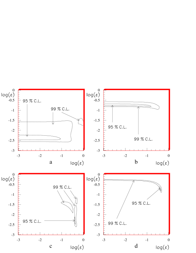
FIG. 1.: Allowed regions in parameter space for a) $\epsilon_{13}$ versus $\epsilon_{22}$, b) $\epsilon_{23}$ versus $\epsilon_{22}$, c) $\epsilon_{13}$ versus $\epsilon_{33}$, and d) $\epsilon_{23}$ versus $\epsilon_{33}$. Both 95 and 99 % C.L. regions are indicated.

TABLE I.: Average distance (in km) traveled by neutrinos through each Earth layer (1=core) for each zenith and momentum bin.

Sample	Bin No.	$\cos\theta$	Layer 1	Layer 2	Layer 3	Layer 4	Layer 5
Sub-GeV	1	$[-1.0,\,-0.6]$	245.0	1780.8	3663.3	630.4	1131.5
	2	$[-0.6,\,-0.2]$	149.4	1130.1	2623.4	505.4	983.7
	3	$[-0.2,\,0.2]$	81.8	649.9	1731.3	373.3	791.1
	4	$[0.2,\,0.6]$	37.6	318.5	1000.0	243.8	565.7
	5	$[0.6,\,1.0]$	10.9	100.9	396.4	112.1	291.6
Multi-GeV	1	$[-1.0,\,-0.6]$	247.5	2148.3	5157.8	811.3	1237.8
	2	$[-0.6,\,-0.2]$	8.2	236.4	2398.9	775.0	1671.9
	3	$[-0.2,\,0.2]$	0.1	12.0	466.8	286.5	1029.4
	4	$[0.2,\,0.6]$	0.0	0.2	34.1	36.1	237.7
	5	$[0.6,\,1.0]$	0.0	0.0	0.4	0.8	11.7

TABLE II.: Fit variables, maximum allowed absolute value derived from the present limits on R-parity violating couplings (assuming $SU(2)_{L}$ symmetry), and lowest $\chi^{2}$ results. The corresponding $\chi^{2}$ value is also given.

Variable	Maximum Absolute Value	Best Fit Value
$\epsilon_{13}$	$0.421.10^{-1}$	$0.45.10^{-2}$
$\epsilon_{23}$	$0.708.10^{-2}$	$0.19$
$\epsilon_{22}$	$0.164$	$0.05$
$\epsilon_{33}$	$0.460$	$0.414$
$\chi^{2}$		$15.6$

TABLE III.: Fit results compared with the data. The first column indicates each of the 13 constraints and the second one gives the observed results: for the solar data the fraction of observed rate over the rate predicted by the Bahcall- Pinsonneault Standard Solar Model 95, and for the atmospheric data the “ratio of ratios” (see text) for each zenith angle bin. The third column shows the predicted results for the model described in this paper.

Solar Neutrinos
Experiment Type	Observed Flux Fraction	Best Fit Flux Fraction
Homestake	$0.273\pm 0.021(exp)\ ^{+0.05}_{-0.03}(theo)$	0.368
Gallium	$0.507\pm 0.049(exp)\pm 0.028(theo)$	0.424
Super-Kamiokande	$0.366\ ^{+0.017}_{-0.014}(exp)\ ^{+0.074}_{-0.046}(theo)$	0.372
Atmospheric Neutrinos
Sub-GeV ($cos\theta$ range)	Observed Ratio of Ratios	Best Fit Ratio of Ratios
$[-1.0,-0.6]$	$0.41\pm 0.07(stat)\pm 0.08(syst)$	0.50
$[-0.6,-0.2]$	$0.63\pm 0.07(stat)\pm 0.08(syst)$	0.50
$[-0.2,0.2]$	$0.63\pm 0.07(stat)\pm 0.08(syst)$	0.58
$[0.2,0.6]$	$0.82\pm 0.07(stat)\pm 0.08(syst)$	0.79
$[0.6,1.0]$	$0.71\pm 0.07(stat)\pm 0.08(syst)$	0.96
Multi-GeV ($cos\theta$ range)	Observed Ratio of Ratios	Best Fit Ratio of Ratios
$[-1.0,-0.6]$	$0.42\pm 0.14(stat)\pm 0.12(syst)$	0.51
$[-0.6,-0.2]$	$0.52\pm 0.13(stat)\pm 0.12(syst)$	0.54
$[-0.2,0.2]$	$0.70\pm 0.12(stat)\pm 0.12(syst)$	0.90
$[0.2,0.6]$	$0.72\pm 0.12(stat)\pm 0.12(syst)$	1.00
$[0.6,1.0]$	$0.87\pm 0.16(stat)\pm 0.12(syst)$	1.00

REFERENCES

- [1] N. Hata and P. Langacker, Phys. Rev. D 56, 6107 (1997).
- [2] Super-Kamiokande Collaboration, Y. Fukuda et al., Phys. Rev. Lett. 81, 1562 (1998). to Phys. Rev. Lett. (1998).
- [3] M. Drees, S.Pakvasa, X.Tata, T. ter Veldhuis, Phys. Rev. D 57, 5335 (1998).
- [4] O.C.W. Kong, hep-ph/9808304 (1998).
- [5] B. Mukhopadhyaya, S. Roy and F. Vissani, hep-ph/9808265 (1998).
- [6] E.J. Chun, S.K. Kang, C.W.Kim and U. W. Lee, hep-ph/9807327 (1998).
- [7] L. Wolfenstein, Phys. Rev. D 17, 2369 (1978).
- [8] S.P. Mikheev and A. Yu. Smirnov, Sov. J. Nucl. Phys. 42, 913 (1985).
- [9] M.M. Guzzo, A. Masiero and S.T. Petcov, Phys. Lett. B 260, 154 (1991).
- [10] E. Roulet, Phys. Rev. D 44, 935 (1991).
- [11] V. Barger, R.J.N. Phillips and K. Whisnant, Phys. Rev. D 44, 1629 (1991).
- [12] P.I. Krastev and J.N.Bahcall, talk given at the Symposium on Flavor Changing Neutral Currents: Present and Future Studies (FCNC 97), Santa Monica, CA, 19-21 Feb 1997.
- [13] J.N. Bahcall and M. Pinsonneault, Rev. Mod. Phys. 67, 781 (1995).
- [14] B. T. Cleveland et al., Proc. of the 7th International Workshop on Neutrino Telescopes, Venice, Feb 27 - Mar 1 1996.
- [15] Sage Collaboration, J.N. Abdurashitov et al., Phys. Lett. B 328, 234 (1994).
- [16] Gallex Collaboration, W. Hampel et al., Phys. Lett. B 388, 384 (1996).
- [17] Super-Kamiokande Collaboration, Y. Fukuda et al., Phys. Rev. Lett. 81, 1158 (1998).
- [18] G.L. Fogli, E. Lisi, A. Marrone and G. Scioscia, hep-ph/9808205 (1998).
- [19] P. Roy, talk given at the Pacific Particle Physics Phenomenology Workshop, Seoul, 31 Oct.-2 Nov., 1997.
- [20] J.E. Kim, P. Ko and D. Lee, Phys. Rev. D 56, 100 (1997).
- [21] MINUIT - Function Minimization and Error Analysis, (CERN Program Library Long Writeup D506), Application Software Group, Computing and Networks Division, CERN, Geneva, Switzerland.
- [22] C. Giunti, C.W. Kim and M. Monteno, hep-ph/9709439 (1997).
- [23] Mathematica 3.0, Copyright 1988-1996 Wolfram Research, Inc.
- [24] S. Bergmann and Y. Grossman, hep-ph/9809524 (1998).