CERN-TH/98-248

UM-TH 98-14

LAPTH 694-98

July 1998

Testing nonperturbative techniques in the scalar sector of the standard model
Adrian Ghinculov^a,b, and Thomas Binoth^c

^aRandall Laboratory of Physics, University of Michigan,
Ann Arbor, Michigan 48109-1120, USA
^bCERN, 1211 Geneva 23, Switzerland
^cLaboratoire d’Annecy-Le-Vieux de Physique Théorique LAPP,
Chemin de Bellevue, B.P. 110, F-74941, Annecy-le-Vieux, France

We discuss the current picture of the standard model’s scalar sector at strong coupling. We compare the pattern observed in the scalar sector in perturbation theory up to two-loop with the nonperturbative solution obtained by a next-to-leading order $1/N$ expansion. In particular, we analyze two resonant Higgs scattering processes, $f\bar{f}\rightarrow H\rightarrow f^{\prime}\bar{f^{\prime}}$ and $f\bar{f}\rightarrow H\rightarrow ZZ,WW$. We describe the ingredients of the nonperturbative calculation, such as the tachyonic regularization, the higher order $1/N$ intermediate renormalization, and the numerical methods for evaluating the graphs.

We discuss briefly the perspectives and usefulness of extending these nonperturbative methods to other theories.

Abstract

We discuss the current picture of the standard model’s scalar sector at strong coupling. We compare the pattern observed in the scalar sector in perturbation theory up to two-loop with the nonperturbative solution obtained by a next-to-leading order $1/N$ expansion. In particular, we analyze two resonant Higgs scattering processes, $f\bar{f}\rightarrow H\rightarrow f^{\prime}\bar{f^{\prime}}$ and $f\bar{f}\rightarrow H\rightarrow ZZ,WW$. We describe the ingredients of the nonperturbative calculation, such as the tachyonic regularization, the higher order $1/N$ intermediate renormalization, and the numerical methods for evaluating the graphs.

We discuss briefly the perspectives and usefulness of extending these nonperturbative methods to other theories.

1 Introduction

The possibility that the electroweak symmetry is broken by a strongly interacting scalar sector received considerable attention in the literature. Interesting scenarios were proposed, such as the possibility of a Higgs boson coupled strongly to the vector bosons and to itself [1], and the formation of a spectrum of bound states at a higher scale which would restore unitarity in scattering processes [2]. Also phenomenological models were proposed for studying quantitatively the implications of strong interactions in the electroweak symmetry breaking sector, such as the BESS model [3].

However, beyond the phenomenological models of strong interactions, an approach based on first principles was missing because of leak of a nonperturbative solution, and of technical difficulties in extending perturbation theory in higher-loop orders. Realistic calculations on a lattice of physical processes involving the Higgs sector are still confronted with technical limitations set, among other issues, by the size of the lattice. $1/N$ expansions in the Higgs sector were only performed at leading order, which is a rather poor approximation. Perturbation theory in the Higgs sector beyond one-loop becomes very difficult because it involves Feynman diagrams with massive internal lines and finite external momenta, for which already at two-loop there are no general analytical solutions available.

Recently, considerable progress has been made in understanding from first principles the nature of the standard Higgs sector when its coupling becomes strong. This is due mainly to technical advances in massive higher-loop techniques and in higher-order nonperturbative $1/N$ expansions. In this paper we would like to discuss the perturbative and nonperturbative aspects of this behaviour at strong coupling.

The major question which will be addressed by future experiments at the LHC is how is the electroweak symmetry broken in nature. While it may or may not turn out to be actually broken by strong, nonperturbative interactions, the Higgs sector remains a fairly simple but not trivial model, where new perturbative and nonperturbative solutions can be tested, in view of applying them to other, possibly more complicated theories.

2 Higher-order perturbation theory

The existing calculations of leading $m_{H}$ radiative corrections in the standard Higgs sector at two-loop level are based on using the equivalence theorem in Landau gauge. This way radiative corrections involve only diagrams with scalars on the internal lines, so that the problem at hand becomes much simpler. This procedure was proposed for the first time in ref. [4], where the one-loop correction to Higgs decay into vector bosons was calculated in this way.

So far at two-loop level the scalar self-energies and the main decay modes of a heavy Higgs boson ($t\bar{t}$, WW, ZZ) are known, and also the high energy limit of vector boson scattering [5]. The vector boson scattering is known completely only at one-loop level [6]. This is due to the complexity of the diagrams involved in a complete two-loop treatment. By using the existing two- and three-point functions, some other scattering processes of phenomenological interest can be derived [7, 9]. For a discussion of the existing results concerning effects of enhanced electroweak strength in the standard model at two-loop order, see for instance ref. [10].

The main decay modes of heavy Higgs bosons are into pairs of vector bosons and into top quark pairs. At leading order, these decay width are given by the following expressions:

$$\Gamma^{(tree)}_{H\rightarrow t\bar{t}} = \frac{3g^{2}}{32\pi}\frac{m_{H}\,m_{t}^{2}}{m_{W}^{2}}\left(1-4\frac{m_{t}^{2}}{m_{H}^{2}}\right)^{3/2}\;\;,$$

$$\Gamma^{(tree)}_{H\rightarrow W^{+}W^{-}} = \frac{g^{2}}{64\pi}\frac{m_{H}^{3}}{m_{W}^{2}}\left(1-4\frac{m_{W}^{2}}{m_{H}^{2}}\right)^{1/2}\left(1-4\frac{m_{W}^{2}}{m_{H}^{2}}+12\frac{m_{W}^{4}}{m_{H}^{4}}\right)\;\;,$$

$$\Gamma^{(tree)}_{H\rightarrow Z^{0}Z^{0}} = \frac{g^{2}}{128\pi}\frac{m_{H}^{3}}{m_{W}^{2}}\left(1-4\frac{m_{Z}^{2}}{m_{H}^{2}}\right)^{1/2}\left(1-4\frac{m_{Z}^{2}}{m_{H}^{2}}+12\frac{m_{Z}^{4}}{m_{H}^{4}}\right)\;\;.$$ (1)

The radiative corrections of enhanced electroweak strength up to two-loop order are given by the following multiplicative factors [5]:

$$\Gamma_{H\rightarrow t\bar{t}}\,=\,\Gamma^{(tree)}_{H\rightarrow t\bar{t}}\,\times\left[1+\lambda\left(\frac{13}{8}-\frac{\pi\,\sqrt{3}}{4}\right)-\lambda^{2}\left(\,.51023\pm 2.5\cdot 10^{-4}\,\right)\right]$$

$$= \Gamma^{(tree)}_{H\rightarrow t\bar{t}}\,\left[1+.264650\,\lambda-\left(\,.51023\pm 2.5\cdot 10^{-4}\,\right)\lambda^{2}\right]$$

$$\Gamma_{H\rightarrow W^{+}W^{-}\,,\,Z^{0}Z^{0}}\,=\,\Gamma^{(tree)}_{H\rightarrow W^{+}W^{-}\,,\,Z^{0}Z^{0}}\,\times$$ (2)

$$\left[1+\lambda\left(\frac{19}{8}+\frac{5\,\pi^{2}}{24}-\frac{3\,\sqrt{3}\,\pi}{4}\right)+\lambda^{2}\left(\,.97103\pm 8.2\cdot 10^{-4}\,\right)\right]$$

$$= \Gamma^{(tree)}_{H\rightarrow W^{+}W^{-}\,,\,Z^{0}Z^{0}}\,\left[1+.350119\,\lambda+\left(\,.97103\pm 8.2\cdot 10^{-4}\,\right)\lambda^{2}\right]\;\;.$$

Here $\lambda=(\frac{g}{4\pi}\frac{m_{H}}{m_{W}})^{2}$ is the quartic coupling of the scalar sector.

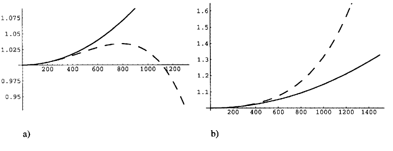
Figure 1: The magnitude of the leading $m_{H}$ radiative corrections to the $H\rightarrow t\bar{t}$ (a) and the $H\rightarrow ZZ,WW$ (b) decays. The plots show the ratios of the decay widths at one-loop (solid line) and two-loop (dashed line) to the tree level decay widths as a function of the on-shell Higgs mass.

In the above expressions, the strength of the coupling of the scalar sector is parameterized by the on-shell Higgs mass $m_{H}$, which is defined by the on-shell renormalization condition $Re\left[P_{HH}^{-1}(s=m_{H}^{2})\right]=0$. We plot the correction factors given by eqns. 2 in figure 1. One can see that for both correction factors the two-loop correction becomes as large as the one-loop correction for $m_{H}$ about 1 TeV (1.1 TeV for $H\rightarrow f\bar{f}$, and 930 GeV for $H\rightarrow WW,ZZ$). Even if the higher-loop corrections are not yet known, this pattern suggests that the radiative corrections blow up strongly around $m_{H}\sim$ 1 TeV. Note that the scheme ambiguities associated with the two-loop result become substantial already for considerable smaller values of the Higgs mass [11]. Of course, similar conclusions can be obtained from other scattering processes apart from the decay modes. This behaviour is in agreement with well-established results regarding perturbative unitarity violation in vector boson scattering at tree level [12].

The point where the perturbative expansion blows up depends on the expansion parameter, and therefore on the renormalization scheme. So far the two-loop results mentioned above were translated into the $\overline{MS}$ [11] and the pole [7, 13] renormalization schemes for processes at the Higgs mass energy scale, in the hope that perturbation theory may show better convergence properties in certain schemes. An overall conclusion of these studies is that the $\overline{MS}$ scheme diverges somewhat sooner and has larger scheme uncertainty than the on-shell scheme, while the pole scheme appears to have slightly better convergence properties than the on-shell scheme. For a more refined discussion of the scheme and gauge dependence see ref. [8]

While the existing higher-order perturbative results in the scalar sector are consistent with a strong blow-up of radiative corrections at about $m_{H}\sim$ 1 TeV, this fact appears somehow puzzling if one considers that the quartic coupling of the scalar sector, $\lambda=(\frac{g}{4\pi}\frac{m_{H}}{m_{W}})^{2}$, is only of order .4 for $m_{H}\sim$ 1 TeV.

From the perspective of the nonperturbative solution to be discussed in the following section, the reason for this behaviour is the Higgs mass saturation effect. Due to the dynamics of the scalar sector, the on-shell Higgs mass is not a good parameterization of the quartic coupling for values larger than $m_{H}\sim$ 1 TeV. However, as will be shown in the following section, at the fundamental level, the scalar sector is perfectly well defined at higher values of the quartic coupling. Well-behaved, unitary solutions can be obtained for various processes by using nonperturbative methods.

At a more speculative level, the fact that the pole scheme seems to show somewhat better convergence properties than the on-shell scheme may have its origin in another nonperturbative property of the Higgs self-energy. This type of nonperturbative effect was discussed in ref. [14] in the context of a theory of vector bosons coupled to a large number of light fermions. The idea is that due to the structure of the self-energy function the on-shell renormalization condition may have no solution for a range of the theory’s coupling, while the pole renormalization condition may have a solution. This results in the on-shell mass being suitable for parameterizing the theory only for a more limited range of the physical coupling than the pole mass. Should such a nonperturbative effect be present in the Higgs sector, this could explain the pattern observed in perturbation theory. In ref. [13] this was investigated by using the nonperturbative $1/N$ expansion, and it was shown that this effect is not present in the Higgs sector of the standard model at LO. It is still an open question if it appears at NLO.

3 Nonperturbative $1/N$ solution

The $1/N$ expansion aims at a nonperturbative solution in order to avoid the problems of perturbation theory at large coupling. Perturbation theory ceases to be a satisfactory solution when radiative correction blow up already at lower loop orders and the renormalization scheme ambiguity is so large that the result becomes unreliable.

The $1/N$ approach is free of these problems because all radiative corrections of all loop orders are explicitly summed up. The idea is to treat the Higgs sector as an $O(N)$-symmetric sigma model, where $N=4$ for the standard model, and to expand in $1/N$ instead of the quartic coupling. The solution is then valid independently of the strength of the coupling — the quality of the approximation depends on the value of $N$. Also it is completely free of renormalization scheme ambiguities. One can work in any intermediate renormalization scheme and still obtain the same result.

Another interesting nonperturbative feature of the $1/N$ expansion of the sigma model is the finiteness of wave function renormalization constants. This is a property of the exact nonperturbative solution, and was checked at next-to-leading order in $1/N$. However, the renormalization of the coupling constants is ultraviolet divergent.

As an extra bonus, the $1/N$ solution provides naturally a consistent treatment of resonant scattering amplitudes. This was known as a long-standing issue in perturbation theory. The essence of the problem is that around a resonance one has to perform a Dyson summation which in perturbation theory at any finite order introduces incomplete higher order contributions which are unphysical. In gauge theories this leads to gauge dependent results. Meanwhile a solution to this problem was found [15, 16], which is based on a Laurent expansion around the physical pole. Within perturbation theory, this solves the problem in a fundamental way, and applies consistently to all orders in perturbation theory. Another approach which was proposed is to use gauge invariant pinch technique self-energies in the Dyson summation. For phenomenological purposes only, other approaches to treat resonant amplitudes were proposed in the literature, which amount to special resummations of low oder results. Some of them may be easier to use in certain phenomenological applications. At the same time they are less fundamental theoretically — some of them still contain unphysical higher order terms, or apply only to tree level or one-loop calculations.

The $1/N$ solution is automatically free of these problems of perturbation theory because it is an all-order solution in the loop expansion.

However, the $1/N$ solution still has some residual ambiguity which can be related to the triviality problem and to possible nondecoupling effects from a hidden heavy sector. Technically, this appears in the tachyonic regularization. Perturbation theory is used at an intermediary stage in the usual $1/N$ treatment, but perturbation theory does not determine the solution uniquely. This is the physical origin of the ambiguity entailed in the tachyonic regularization.

3.1 $1/N$ combinatorial rearrangement and diagrammatics

We start with the usual Lagrangean of a $O(N)$-symmetric sigma model:

$${\cal L}_{1}=\frac{1}{2}\partial_{\nu}\Phi_{0}\partial^{\nu}\Phi_{0}-\frac{\mu_{0}^{2}}{2}\Phi_{0}^{2}-\frac{\lambda_{0}}{4!N}\Phi_{0}^{4}~{}~{},~{}~{}\Phi_{0}\equiv\left(\phi_{0}^{1},\phi_{0}^{2},\dots,\phi_{0}^{N}\right)$$ (3)

From this Lagrangean one can in principle derive directly a perturbative expansion for Green functions, and classify the Feynman diagrams according to their order in $1/N$. However, beyond leading order the combinatorics becomes very complicated. In order to perform explicit calculations beyond leading order it is useful to perform a rearrangement of perturbation theory. A useful trick for doing this was proposed in ref. [17]. It consists of adding a nondynamical term to the Lagrangean:

$${\cal L}_{2} = {\cal L}_{1}+\frac{3N}{2\lambda_{0}}(\chi_{0}-\frac{\lambda_{0}}{6N}\Phi_{0}^{2}-\mu_{0}^{2})^{2}$$ (4)

$$= \frac{1}{2}\partial_{\nu}\Phi_{0}\partial^{\nu}\Phi_{0}-\frac{1}{2}\chi_{0}\Phi_{0}^{2}+\frac{3N}{2\lambda_{0}}\chi_{0}^{2}-\frac{3\mu_{0}^{2}N}{\lambda_{0}}\chi_{0}+const.$$

This involves the introduction of an unphysical auxiliary field $\chi$. As one can see, the equation of motion for $\chi$ is just an equation of constraint, and therefore the physical spectrum and the dynamics of the model remain unchanged. The effect of this trick is that the Feynman rules are changed. Namely, the quartic couplings are eliminated. The only vertices left are trilinear, and involve one $\chi$ field and two physical scalars. This simplifies enormously the combinatorics of Feynman graphs in higher orders.

We note that some other rearrangement schemes with different properties were discussed for the $O(N)$-symmetric sigma model in ref. [18]. To our best knowledge, these schemes were not applied so far in actual calculations.

In the following we describe the counterterm structure which is used for performing renormalization at NLO in the $1/N$ expansion. A somewhat different approach is presented in ref. [19], but the final results are the same.

Renormalization is performed in principle order by order in perturbation theory. However, for performing actual calculations of higher order in $1/N$, it is of advantage to group all counterterms of various loop orders and which are of the same $1/N$ order into the same $1/N$ counterterm. We define the $1/N$ counterterms as follows:

$$\frac{3}{\lambda_{0}} = \frac{3}{\lambda}+\Delta\lambda~{}~{}~{}~{}~{}~{}~{}~{}~{}~{}~{}\equiv~{}~{}\frac{3}{\lambda}+\delta\lambda^{(0)}+\frac{1}{N}\delta\lambda+{\cal O}\left(\frac{1}{N^{2}}\right)$$

$$\frac{3\mu_{0}}{\lambda_{0}} = -\frac{v^{2}}{2}(1+\Delta t)~{}~{}~{}\equiv~{}~{}-\frac{v^{2}}{2}\left[1+\frac{1}{N}\delta t+{\cal O}\left(\frac{1}{N^{2}}\right)\right]$$

$$\phi^{i}_{0} = \pi_{i}Z_{\pi}~{}~{}~{}~{}~{}~{}~{}~{}~{}~{}~{}~{}~{}~{}~{}\,\equiv~{}~{}\pi_{i}\left[1+\frac{1}{N}\delta Z_{\pi}+{\cal O}\left(\frac{1}{N^{2}}\right)\right]~{},~{}~{}i=1,\dots,N-1$$

$$\phi^{N}_{0} = \sigma Z_{\sigma}+\sqrt{N}v~{}~{}~{}~{}~{}~{}\equiv~{}~{}\sigma\left[1+\frac{1}{N}\delta Z_{\sigma}+{\cal O}\left(\frac{1}{N^{2}}\right)\right]+\sqrt{N}v$$

$$\chi_{0} = \chi Z_{\chi}+\hat{\chi}+\Delta t_{\chi}~{}~{}\equiv~{}~{}\chi\left(1+\frac{1}{N}\delta Z_{\chi}\right)+\frac{v^{2}}{N}\delta t_{\chi}+{\cal O}\left(\frac{1}{N^{2}}\right)$$ (5)

Here we already used the fact that the tadpole and wave function renormalization counterterms do not receive contributions at leading order in $1/N$. We also note that although two tadpole counterterms are present, $\delta t$ and $\delta t_{\chi}$, they are related through the gap equation [20], for instance by requesting that the leading order ground state condition $\hat{\chi}=0$ be preserved in higher orders, where $\hat{\chi}$ is the vacuum expectation value of the $\chi$ field in the spontaneously broken phase.

At this point it is useful to note that since the two Lagrangeans of eqns. 3 and 4 are equivalent, a linear combination will also describe the same physics. This observation can be exploited for performing BPHZ renormalization in a more elegant way, as will be explained in the following. Beyond leading order in $1/N$ it is advantageous to work with a linear combination of the potential parts of Lagrangeans ${\cal L}_{1}$ and ${\cal L}_{2}$. Keeping only the contributions relevant for next-to-leading order calculations, we consider in fact the following Lagrangean:

$${\cal L}_{3} = \frac{1}{2}(\partial_{\mu}\vec{\pi})(\partial^{\mu}\vec{\pi})\left[1+\frac{2}{N}\delta Z_{\pi}\right]+\frac{1}{2}(\partial_{\mu}\sigma)(\partial^{\mu}\sigma)\left[1+\frac{2}{N}\delta Z_{\sigma}\right]$$ (6)

$$+\chi^{2}\frac{N}{2}\left\{\frac{3}{\lambda}+\delta\lambda^{(0)}+\frac{1}{N}\left[\delta\lambda+2\left(\frac{3}{\lambda}+\delta\lambda^{(0)}\right)\delta Z_{\chi}\right]\right\}$$

$$-\chi\sigma\sqrt{N}v\left[1+\frac{1}{N}\left(\delta Z_{\chi}+\delta Z_{\sigma}\right)\right]$$

$$-\frac{1}{2}\left(\vec{\pi}^{2}+\sigma^{2}\right)\frac{v^{2}}{N}\delta t_{\chi}$$

$$-\frac{1}{2}\chi\vec{\pi}^{2}\left[1+\frac{1}{N}\left(\delta Z_{\chi}+2\delta Z_{\pi}\right)\right]$$

$$-\frac{1}{2}\chi\sigma^{2}\left[1+\frac{1}{N}\left(\delta Z_{\chi}+2\delta Z_{\sigma}\right)\right]$$

$$-\sigma\frac{v^{3}}{\sqrt{N}}\delta t_{\chi}+\chi v^{2}\left[\left(\frac{3}{\lambda}+\delta\lambda^{(0)}\right)\delta t_{\chi}+\frac{1}{2}\delta t+\frac{1}{2N}\delta t\;\delta Z_{\chi}\right]$$

$$+\frac{K}{N^{2}}\left[4Nv^{2}\sigma^{2}+\left(\vec{\pi}^{2}\right)^{2}+\sigma^{4}+2\vec{\pi}^{2}\sigma^{2}+4\sqrt{N}v\sigma\left(\vec{\pi}^{2}+\sigma^{2}\right)\right]$$

Here $K$ is in principle a completely arbitrary constant. We have the freedom to choose it so that actual calculations are more convenient. We will consider $K$ to be of order 1 in the $1/N$ expansion. Thus the potential part of ${\cal L}_{2}$ is regarded as an ${\cal O}(1/N)$ counterterm. We will choose the actual value of $K$ so that the renormalization procedure is more transparent at NLO in the $1/N$ expansion.

The Feynman rules can be read out directly from the above expression. Within this diagrammatical rearrangement of the sigma model, counting powers of $1/N$ in multiloop diagrams is straightforward: closed Goldstone loops contribute a factor $N$, while $\chi\chi$ propagators give a $1/N$ factor, and mixed $\chi\sigma$ propagators contribute $1/\sqrt{N}$. At the same time, the absence of quartic couplings at tree level reduces considerably the number of possible topologies.

For these reasons, for a given process and a given order in $1/N$, it is easy to write down the Feynman graphs of all loop orders. As it will become clear from the discussion of two- and three-point functions, there is always a finite number of multiloop topologies, where one can only insert chains of one-loop bubbles in the $\chi\chi$ and $\chi\sigma$ propagators without increasing the $1/N$ order of the graph.

We emphasize that this combinatorial rearrangement of the sigma model is quite crucial. It is possible to calculate explicitly nonperturbative processes in the Higgs sector precisely because the combinatorial rearrangement enables one to write down explicitly and in a manageable way the diagrams of all loop orders, without truncating the perturbative expansion.

3.2 Tachyonic regularization

It is straightforward to derive the two-point functions of the theory at leading order in $1/N$. This was done for instance in ref. [17]. The only diagram involved is the one-loop bubble diagram shown in figure 2. One finds the following leading order propagators:

$i(N-1)\hat{\alpha}^{(0)}(s)$	$=$		+	counterterm

Figure 2: The leading order bubble diagram.

$$D_{\sigma\sigma}(s) = \frac{i}{s-m^{2}(s)}$$

$$D_{\chi\chi}(s) = \frac{1}{Nv^{2}}\frac{ism^{2}(s)}{s-m^{2}(s)}$$

$$D_{\chi\sigma}(s) = \frac{1}{\sqrt{N}v}\frac{im^{2}(s)}{s-m^{2}(s)}$$

$$D_{\pi_{i}\pi_{j}}(s) = \frac{i}{s}\delta_{ij}$$ (7)

where

$$m^{2}(s)=\frac{v^{2}}{\frac{3}{\lambda}+\hat{\alpha}^{(0)}(s)}~{}~{}~{}~{}~{}\equiv~{}~{}~{}~{}~{}\frac{v^{2}}{\frac{3}{\lambda}-\frac{1}{32\pi^{2}}\log{\left(-\frac{s+i\eta}{\mu^{2}}\right)}}$$ (8)

Here $\hat{\alpha}^{(0)}(s)\equiv\alpha^{(0)}(s)+\delta\lambda^{(0)}$ is the ultraviolet finite part of the self-energy diagram of fig. 1, and $\mu$ is the subtraction scale.

In the expressions above, apart from the expected Higgs pole, one notices the presence of a tachyonic pole. It appears at an energy $s=-\Lambda_{t}^{2}$ which is given by the following transcendental equation:

$$\frac{v^{2}}{\Lambda_{t}^{2}}-\frac{1}{32\pi^{2}}\log{\left(\frac{\Lambda_{t}^{2}}{\mu^{2}}\right)}+\frac{3}{\lambda}=0~{}~{}~{}~{}~{}.$$ (9)

The tachyon scale $\Lambda_{t}$ differs from the Landau scale $\Lambda_{L}=\mu e^{48\pi^{2}/\lambda}$ by a shift of order $v^{2}/\Lambda_{L}^{2}$.

The leading order tachyon is a well-known difficulty of the $1/N$ nonperturbative treatment of the sigma model. From the technical point of view, it induces causality violating effects in the theory. As long as one is concerned only with the leading order, one can try to make sense of the result by limiting its validity to an energy range considerably smaller than the tachyon scale. However, there is no such easy way out for calculations beyond leading order because the tachyon appears then in loops.

One way to circumvent this is by making the assumption that the tachyon indicates the triviality of the theory. This sets a limit for the validity of the $1/N$ result at high energy. At some energy scale new physics sets in. This scale is presumably of the order of the tachyon scale, but not necessarily equal or lower. Then an obvious treatment is to introduce a cutoff in the loop integrations [21]. This is then interpreted as a model of nondecoupling effects from an unknown heavy sector. However, in this approach the momentum cutoff has to be lower than the tachyon scale, which is necessary for computational purposes only and is not motivated physically. Also a loop momentum cutoff spoils the gauge invariance of the gauged model. It also introduces quadratic dependencies on the cutoff scale and these are known in effective theories not to be directly related to heavy mass effects — actually counterexamples were found in the literature in two-loop calculations [22].

We use a different treatment of the tachyonic pole [23], which is more convenient for higher order calculations in the $1/N$ expansion. We subtract the tachyon minimally at its pole, which means using the following propagators instead of those of eqns. 7:

$$D_{\sigma\sigma}(s) = i\left[\frac{1}{s-m^{2}(s)}-\frac{\kappa}{s+\Lambda_{t}^{2}}\right]$$

$$D_{\chi\chi}(s) = \frac{is}{Nv^{2}}\left[\frac{m^{2}(s)}{s-m^{2}(s)}+\frac{\kappa\Lambda_{t}^{2}}{s+\Lambda_{t}^{2}}\right]$$

$$D_{\chi\sigma}(s) = \frac{i}{\sqrt{N}v}\left[\frac{m^{2}(s)}{s-m^{2}(s)}+\frac{\kappa\Lambda_{t}^{2}}{s+\Lambda_{t}^{2}}\right]~{}~{}~{}~{}~{},$$ (10)

were

$$\kappa=\frac{1}{1+\frac{\Lambda_{t}^{2}}{32\pi^{2}v^{2}}}$$ (11)

is the residuum of the tachyonic pole.

The justification of the tachyonic regularization introduced above is the following. Green functions — such as the two-point functions above — are calculated in the $1/N$ expansion starting with the perturbative expansion in the coupling constant $\lambda$ of the coefficients of the $1/N$ expansion. Then, all Feynman graphs of all loop orders which contribute to a given order in $1/N$ are calculated explicitly and summed up. Since the $1/N$ coefficient is only known as a power series in $\lambda$ to start with, it will be determined by its perturbative expansion up to a function of $\lambda$ which vanishes identically in perturbation theory, of the type $e^{1/\lambda}$. Since the residuum of the tachyon is such a function whose perturbative expansion vanishes, its presence cannot be taken seriously as a prediction of the theory and as an indication that the theory is ill-defined. While the $\lambda\phi^{4}$ theory is widely believed to be trivial, the tachyon in the $1/N$ expansion is certainly not a rigorous proof thereof.

When we use the minimal tachyon subtraction scheme of eqns. 10, we effectively use the freedom to add a function which vanishes in perturbation theory for restoring the causality of the theory. In this sense, our treatment is independent of whether one regards the theory as being an effective one or not. If one takes the view that the theory is trivial and wants to include nondecoupling effects from a heavy sector, such effects can be superimposed over the whole calculation. Compared to a naive cutoff, this tachyonic regularization does not require the heavy sector to be strictly under the tachyon scale.

3.3 Nonperturbative two- and three-point functions at NLO

Beyond leading order in $1/N$, actual calculations have to be performed numerically because in general the multiloop diagrams involved are not manageable analytically. This brings about some technical complications related to the treatment of ultraviolet divergencies in conjunction with numerical integration.

A useful observation is that the final result in the $1/N$ expansion is free of any renormalization scheme ambiguity. This is because it is exact at all orders in the coupling constant. This leaves us the freedom of working in any intermediate renormalization scheme at our convenience, since the final result is independent of that. This can be best exploited for simplifying to some extent the numerical work.

$i\alpha(s)$	$=$		$A_{1}$	$+$	$A_{2}$	$+$	$A_{3}$
		$+$	$A_{4}$	$+$	$A_{5}$
$i\frac{v^{2}}{N}\beta(s)$	$=$		$B_{1}$	$+$	$B_{2}$
$i\frac{v}{\sqrt{N}}\gamma(s)$	$=$		$C_{1}$	$+$	$C_{2}$
$i\frac{v^{2}}{N}\delta(s)$	$=$		$D$
T	$=$
- $i\frac{v}{N\sqrt{N}}\eta(s)$	$=$		$E_{1}$
- $i\frac{1}{N}\phi(s)$	$=$		$F_{1}$	$+$	$F_{2}$	$+$	$F_{3}$

Figure 3: Infinite sums of multiloop Feynman diagrams which contribute in next-to-leading order in $1/N$ to the two- and three-point functions of the $O(N)$ sigma model. The blob on propagators denotes the summed-up leading order propagators. Note that the $\pi\pi$ propagator at leading order in $1/N$ is a free propagator. One of the graphs above is shown in expanded form in fig. 4.

The graphs needed for the calculation of all two- and three-point functions of the theory at next-to-leading order in $1/N$ are shown in fig. 3. In addition to the two- and three-point graphs, there is also one tadpole graph which is needed for the determination of the tadpole counterterm $\delta t_{\chi}$. Each graph is in fact a sum of multiloop Feynman graphs which are all of the same order in $1/N$, and of various orders in the coupling constant $\lambda$. This is shown explicitly for one particular self-energy graph in fig. 4.

$iA_{1}(s)=$

$$\equiv~{}~{}\sum_{k=0}^{\infty}\sum_{l=0}^{\infty}$$

Figure 4: Multiloop diagrams with three-loop topology which contribute to the $\chi\chi$ propagator in next-to-leading order.

The graphs involved, $A_{i}$, $B_{i}$, $C_{i}$, $D_{i}$, $E_{i}$, $F_{i}$ and $T$, are in general ultraviolet divergent. Since our strategy is to calculate them numerically, we first subtract the divergencies and subdivergencies of these graphs. An inspection of the Feynman diagrams which compose each graph of figure 3 reveals that the ultraviolet divergencies are polynomial, just as if they were usual Feynman diagrams, and in spite of the infinite number of loops involved. We define in figures 5, 6 and 7 a set of ultraviolet subtracted graphs, $\hat{A}_{i}$, $\hat{B}_{i}$, $\hat{C}_{i}$, $\hat{D}_{i}$, $\hat{E}_{i}$, and $\hat{F}_{i}$. They are finite, and thus can be calculated by direct numerical integration.

$i\hat{A}_{4}(s)~{}=$			$-$
	$-~{}2\times$		$+~{}2\times$		$-$	overall subtraction
$i\hat{A}_{2}(s)~{}=$			$-$
$i\hat{A}_{3}(s)~{}=$			$-$
	$-$	$\partial$	$-$	overall subtraction
$i\hat{A}_{4}(s)~{}=$			$-~{}2\times$
	$-$		$+~{}2\times$		$-$	overall subtraction
$i\hat{A}_{5}(s)~{}=$			$-$
	$-$		$+$

Figure 5: Definition of the subtracted $\chi\chi$ self-energy graphs. The symbol $\partial$ indicates the differentiation with respect to the external momentum of the box.

$i\frac{v^{2}}{N}\hat{B}_{1}(s)~{}=$			$-$		$-$	$\partial$
$i\frac{v^{2}}{N}\hat{B}_{2}(s)~{}=$			$-$
$i\frac{v}{\sqrt{N}}\hat{C}_{1}(s)~{}=$			$-$
$i\frac{v}{\sqrt{N}}\hat{C}_{2}(s)~{}=$			$-$
	$-$		$+$
$i\frac{v^{2}}{N}\hat{D}(s)~{}=$			$-$		$-$	$\partial$

Figure 6: Definition of the subtracted $\sigma\sigma$, $\chi\sigma$ and $\pi\pi$ self-energy graphs.

$i\frac{v}{\sqrt{N}}\hat{E}_{1}(s)$	$=$			$-$
$i\frac{v}{\sqrt{N}}\hat{F}_{1}(s)$	$=$			$-$
$i\frac{v}{\sqrt{N}}\hat{F}_{2}(s)$	$=$			$-$
$i\frac{v}{\sqrt{N}}\hat{F}_{3}(s)$	$=$			$-$
		$-$		$+$

Figure 7: Definition of the subtracted vertex graphs.

The numerical evaluation of the ultraviolet finite, subtracted graphs is done by using a numerical method for the calculation of massive three-loop Feynman diagrams [24]. This method reduces all subtracted graphs to a two-dimensional integral representation. After an appropriate rotation of the integration path in the complex plane, these two-dimensional integrals can be evaluated numerically [23].

The subtracted graphs are used further for calculating physical amplitudes. Here we consider the scattering processes $f\bar{f}\rightarrow H\rightarrow f^{\prime}\bar{f^{\prime}}$ and $f\bar{f}\rightarrow H\rightarrow ZZ,WW$. Phenomenologically they are important as a Higgs production mechanism at a possible muon collider. Also the heavy Higgs effects in these scattering processes are related to those in the gluon fusion process, which is the main Higgs production mechanism at the LHC.

To start with, we consider the matrix element for the fermion scattering process $f\bar{f}\rightarrow H\rightarrow f^{\prime}\bar{f^{\prime}}$ at leading order in the fermion mass. Then, the correction to the $Hf\bar{f}$ vertex is given simply by the ratio of the wave function renormalization factors $Z_{\sigma}/Z_{\pi}$, because true vertex diagrams are of higher order in the fermion mass. The calculation reduces essentially to evaluating the Higgs propagator. Up to the overall factor from the tree level Yukawa couplings, the amplitude is given by the following expression, were we included the relevant counterterms in addition to the pure $1/N$ multiloop graphs of fig. 3:

$${\cal M}_{f\bar{f}} = \frac{1}{s-m^{2}(s)\left[1-\frac{1}{N}f_{1}(s)\right]}$$

$$f_{1}(s) = \frac{m^{2}(s)}{v^{2}}\left[\alpha(s)+\delta\lambda+2\frac{v^{2}}{m^{2}(s)}\delta Z_{\chi}+8K\alpha_{0}^{2}(s)+2\alpha_{0}(s)\delta Z_{\pi}\right]$$ (12)

$$+2\left[\gamma(s)-\delta Z_{\chi}-8K\alpha_{0}(s)\right]+\frac{v^{2}}{m^{2}(s)}\left[\beta(s)-\delta t_{\chi}+8K+2\frac{s}{v^{2}}\delta Z_{\pi}\right]$$

One can easily see in the above expression that one could have done without a wave function renormalization for the unphysical $\chi$ field, and also without the $K$ counterterm which was introduced in eq. 6 only for convenience purposes. It can be seen easily that these terms cancel out trivially in the expression above. In fact, since there is no Higgs external leg in the process considered, it is also unnecessary to introduce a wave function renormalization for the $\sigma$ field.

As we discussed in section 3.1, these counterterms are only introduced for convenience. If one cancels out these spurious terms in the expression above, one is left with a sum of multiloop diagrams which are individually ultraviolet divergent. Since the whole expression is a physical quantity, the ultraviolet divergencies cancel out among the multiloop diagrams. However, the actual cancellation pattern is not very transparent due to the complexity of the diagrams. Because we need to calculate the $1/N$ graphs numerically, we need the expressions to be ultraviolet convergent. At the same time it is very complicated to extract the ultraviolet divergencies and subdivergencies from the graphs of fig. 3 as $1/\epsilon$ poles, as it is done in usual Feynman diagrams. In more complicated processes, such as three- and four-point processes, the cancellation is even more involved.

The $K$ and $\delta Z_{\chi}$ counterterms serve as vehicles of the ultraviolet cancellations among the multiloop diagrams. For this purpose we assign to these two counterterms the following expressions:

$$K = -\frac{1}{4}B_{2}(0)$$

$$\delta Z_{\chi} = C_{1}(0)+C_{2}(0)+2B_{2}(0)\alpha_{0}(\mu^{2}\rightarrow 0)~{}~{}~{}~{}~{}~{},$$ (13)

and also we note the identity:

$$\delta t_{\chi}=B_{1}(0)-B_{2}(0)~{}~{}~{}~{}~{}~{}.$$ (14)

Then the actual multiloop $1/N$ graphs from $\alpha$, $\beta$ and $\gamma$ combine with the counterterms and give precisely the subtracted multiloop graphs $\hat{A}_{i}$, $\hat{B}_{i}$ and $\hat{C}_{i}$ defined in figures 5 and 6:

$$f_{1}(s)=\frac{m^{2}(s)}{v^{2}}\left[\hat{\alpha}(s)+\delta\lambda^{fin.}\right]+2\hat{\gamma}(s)+\frac{v^{2}}{m^{2}(s)}\left[\hat{\beta}(s)-2\frac{s-m^{2}(s)}{v^{2}}\left(\delta Z_{\sigma}-\delta Z_{\pi}\right)\right]$$ (15)

Actually the finite term $\left(\delta Z_{\sigma}-\delta Z_{\pi}\right)$ in this expression simply means that one has to subtract the momentum derivative of diagram $D(s)$ from diagram $B_{1}(s)$, rather than the derivative of $B_{1}(s)$, as defined in figure 6. The finite contribution $\delta\lambda^{fin.}$ which is left in eq. 15 simply reminds that for specifying the strength of the coupling of the theory, a mass scale needs to be given along with the value of $\lambda$. A shift in $\delta\lambda^{fin.}$ can be absorbed into a shift in the subtraction point $\mu$. As such, $\delta\lambda^{fin.}$ can be shifted to zero.

Along the same lines, the following expression is obtained for the amplitude of the $f\bar{f}\rightarrow H\rightarrow ZZ,WW$ scattering process:

$${\cal M}_{WW} = \frac{m^{2}(s)}{\sqrt{N}v}\frac{1-\frac{1}{N}f_{2}}{s-m^{2}(s)\left[1-\frac{1}{N}f_{1}(s)\right]}$$

$$f_{1}(s) = \frac{m^{2}(s)}{v^{2}}\,\hat{\alpha}(s)+2\hat{\gamma}(s)+\frac{v^{2}}{m^{2}(s)}\left[\hat{\beta}(s)-2\frac{s-m^{2}(s)}{v^{2}}\left(\delta Z_{\sigma}-\delta Z_{\pi}\right)\right]$$

$$f_{2}(s) = \frac{m^{2}(s)}{v^{2}}\,\hat{\alpha}(s)+\hat{\gamma}(s)-\hat{\phi}(s)-\frac{v^{2}}{m^{2}(s)}\hat{\eta}(s)$$ (16)

All quantities involved in this expression, $\hat{\alpha}$, $\hat{\beta}$, $\hat{\gamma}$, $\hat{\eta}$, and $\hat{\phi}$, are sums of the subtracted graphs defined in figures 4, 5 and 6. They can be calculated directly by numerical integration [23, 19].

3.4 The saturation effect

The shape of the Higgs resonance can be obtained nonperturbatively in the quartic Higgs coupling at next-to-leading order in the $1/N$ expansion by evaluating numerically the expressions for ${\cal M}_{f\bar{f}}$ and ${\cal M}_{WW}$ given in the previous section. These two scattering processes are the main production and decay modes for the Higgs boson at a possible muon collider. Also these processes are related to Higgs production by gluon fusion [9]. This is the main production mechanism at hadron colliders such as the LHC.

We give in figure 8 the resulting line shapes of the Higgs resonance. One feature of these line shapes is that they agree remarkably well with the perturbative results for low couplings. The next-to-leading order $1/N$ results are very close to the two-loop perturbation theory line shapes for $m_{H}$ up to about 800–900 GeV. The agreement confirms the consistency of the $1/N$ approach in higher orders and establishes that the next-to-leading oder is an excellent approximation.

Figure 8: The line shape of the Higgs resonance in the scattering processes $f\bar{f}\rightarrow H\rightarrow f^{\prime}\bar{f^{\prime}}$ and $f\bar{f}\rightarrow H\rightarrow ZZ,WW$. We marked the position of the maxima of the resonances (solid line for the $1/N$ result and dashed line for the perturbative result at two-loop).

At higher quartic coupling a saturation effect sets in. The maximum of the resonance does not shift towards higher energy, the resonance only becomes wider. To make this effect clearer, we extract some mass ($M_{peak}$) and width ($\Gamma_{peak}$) variables from the position and the height of the resonance in fermion scattering. The definition of the variables $M_{peak}$ and $\Gamma_{peak}$ is the following. We determined numerically the position and the height of the maximum of the resonance. Then, $M_{peak}$ and $\Gamma_{peak}$ are the mass and width of a Breit-Wigner resonance which has the same height and position of the peak. Of course, the actual Higgs lineshapes are not exactly of Breit-Wigner type. However, $M_{peak}$ and $\Gamma_{peak}$ describe reasonably well the main features of the resonance. We compare in figure 9 the $M_{peak}$ – $\Gamma_{peak}$ relation with the perturbative result. Of course one is free to choose any other parameterization of the resonance, but the $M_{peak}$ and $\Gamma_{peak}$ variables which we use here are sufficient for comparing with perturbation theory.

Figure 9: The saturation effect in the $f\bar{f}\rightarrow H\rightarrow f^{\prime}\bar{f^{\prime}}$ scattering. The mass and width variables $M_{peak}$ and $\Gamma_{peak}$ are related to the position and the height of the Higgs resonance as explained in the text.

As one can see in figure 8, the saturation effect is present in the $f\bar{f}\rightarrow H\rightarrow ZZ,WW$ scattering process as well, at a comparable energy. The precise maximum position of the peak is process dependent because the resonance shape is deformed by the energy dependence of different contributions, such as the vertex corrections in this case. A universal way of parameterizing the saturation effect would be by using the pole mass and width of the Higgs particle. Extracting this in the next-to-leading $1/N$ approach is numerically more difficult because the subtracted $1/N$ graphs need to be continued into the second Riemann sheet for solving the pole equation. This is not available yet.

The saturation effect provides more insight in the way perturbation theory breaks down and radiative corrections blow up in the Higgs sector. The dramatical failure of perturbation theory at around 1 TeV is well-established by tree level unitarity violations [12]. Higher order radiative corrections blow up at a similar scale, as was discussed in section 2. Less violent problems can show up in the form of considerable scheme ambiguities of the results. At the same time however, it is puzzling that at the 1 TeV scale the quartic coupling is numerically not exceedingly large yet. The quartic coupling only becomes of the order of unity when the tree level on-shell Higgs mass is of the order of 1.5 TeV. Naively this is where one would expect heavy problems for perturbation theory to set in. From the perspective of the saturation effect, the explanation is clear now. The mass of the Higgs boson is not a good expansion parameter beyond the saturation point. In the saturation region the mass does not increase when the coupling is enhanced. In fact, the width of the resonance as a function of the mass is a double valued function. The well-known perturbation theory results break down at about 1 TeV because of the use of a bad expansion parameter. For that region the width would be a more appropriate parameterization of the coupling than the mass.

4 Nonperturbative solutions of other theories: $1/N$ QED

In this section we would like to comment briefly on the perspectives of extending this kind of nonperturbative methods to solving other field theories of physical interest.

We already mentioned that the applicability of the nonperturbative $1/N$ expansion, especially in higher orders, depends crucially on the particular theory under consideration. One needs to arrange the perturbative expansion of the theory in such a way that the various loop contributions can be sorted out by powers of $1/N$ in a manageable way, so that the graphs of all loop-orders can be explicitly calculated and summed up for a given order of $1/N$.

Such a theory where the rearrangement of perturbation theory is straightforward is the ordinary QED. QED can be seen as an example where the $1/N$ expansion works poorly because the value of $N$ is too small. The existing calculations in perturbative QED are rather advanced, the coupling constant is small, and therefore the $1/N$ treatment of QED can hardly compete with the perturbative treatment. Here we will briefly discuss a simple leading order $1/N$ QED calculation for comparing with perturbation theory, and see in which cases a $1/N$ treatment can be superior to perturbation theory.

QED can be organized as a $1/N$ expansion by introducing $N$ species of electrons and at the same time dividing the gauge coupling by $\sqrt{N}$. Then one sees immediately that the counting of powers of $1/N$ proceeds similarly as in the case of the sigma model. Ordinary QED is recovered in the limit $N=1$. Already at this point one can expect the convergence of the $1/N$ expansion to be poor because of the value of the expansion parameter.

Figure 10: Diagrams which contribute to the anomalous magnetic moment of the electron in leading order of the $1/N$ expansion.

We show in figure 10 the Feynman diagrams which contribute to the anomalous magnetic moment of the electron in leading order of $1/N$. They are the same diagrams discussed in ref. [25] in the context of the large order behaviour of QED. We refer to this work for details on the calculation of the contributions to the anomalous magnetic moment due to these diagrams. The equivalent of the tachyonic regularization in the $O(N)$-symmetric sigma model is the subtraction in the loop momentum integration of the diagrams of figure 10 of a term of the type $e^{1/\alpha}$, which vanishes in perturbation theory, as discussed in ref. [25]. Note that due to the value of the coupling constant, in QED the Landau pole is at a very high energy scale.

The perturbative results for the anomalous magnetic moment of the electron up to four-loop are [26]:

$$a_{1-loop} = .5$$

$$a_{2-loop} = -.328478965$$

$$a_{3-loop} = 1.181241$$

$$a_{4-loop} = -1.557~{}~{}~{}~{},$$ (17)

and their contribution to the anomalous magnetic moment is $\Sigma_{n}\,a_{n}(\alpha/\pi)^{n}$.

By numerical integration one can calculate the LO contribution in the $1/N$ expansion to the anomalous magnetic moment of the electron. The result is $a^{LO~{}1/N}=.001161494$. The first few terms in the loop expansion of this result are:

$$a^{LO~{}1/N}_{1-loop} = .5$$

$$a^{LO~{}1/N}_{2-loop} = .015687421$$

$$a^{LO~{}1/N}_{3-loop} = .002558524$$

$$a^{LO~{}1/N}_{4-loop} = .000876865$$

$$a^{LO~{}1/N}_{5-loop} = .000470905$$

$$a^{LO~{}1/N}_{6-loop} = .000344687$$

$$a^{LO~{}1/N}_{7-loop} = .000318119$$

$$a^{LO~{}1/N}_{8-loop} = .000352804$$

$$a^{LO~{}1/N}_{9-loop} = .000455370$$

$$a^{LO~{}1/N}_{10-loop} = .000668824$$

$$a^{LO~{}1/N}_{11-loop} = .001099482$$

$$a^{LO~{}1/N}_{12-loop} = .001997590$$

$$a^{LO~{}1/N}_{13-loop} = .003971440~{}~{}~{}~{},$$ (18)

such that their contribution to the anomalous magnetic moment is $\Sigma_{n}\,a^{LO~{}1/N}_{n}(\alpha/\pi)^{n}$. The numbers above agree with the results given in ref. [25].

By comparing the LO $1/N$ result with perturbation theory, one sees that this is only marginally different from the one-loop perturbative result. Comparing the perturbative expansion of the LO $1/N$ result (eqns. 18) and the perturbation theory result (eqns. 17), it can be seen that the LO $1/N$ Feynman diagrams are not numerically the main contribution from higher-loop orders in perturbation theory.

This shows that the usefulness of the $1/N$ expansion versus perturbation theory depends crucially on the value of $N$ and of the coupling constant. If $N$ is large enough, the other diagrams appearing in higher-order perturbation theory besides those included in the $1/N$ expansion will be suppressed by powers of $1/N$. This way the $1/N$ expansion can converge faster than perturbation theory. If the coupling constant is large, perturbation theory starts to diverge already at low orders and the scheme ambiguities may prevent one to obtain the desired accuracy. Then the $1/N$ expansion is expected to be a better alternative because it is free of scheme ambiguities and the solution is valid for strong coupling as well.

Therefore it is not surprising that the $1/N$ expansion works so well in heavy Higgs physics, where $N=4$ and $\lambda$ is of order 1.

Extending these computational tools in the case of nonabelian gauge theories is very difficult because of the presence of trilinear and quartic couplings of the gauge bosons. In the case of QCD the topological structure of the graphs which appear in the $1/N_{c}$ expansion is known [27], but so far they could not be calculated explicitly in four dimensions. The well-known solution of QCD in two dimensions [28] was possible because in this case the quartic and trilinear couplings are absent, which reduces the types of topologies of Feynman graphs appearing in higher loop orders.

5 Conclusions

We investigated in some detail the scalar sector of the standard model at strong coupling. For doing this we used both perturbation theory up to two-loop order and a nonperturbative treatment within the next-to-leading order $1/N$ expansion. With these approaches we treated the main heavy Higgs decay modes as well as two scattering processes where the Higgs line shape can be observed, $f\bar{f}\rightarrow H\rightarrow f^{\prime}\bar{f^{\prime}}$ and $f\bar{f}\rightarrow H\rightarrow ZZ,WW$. These two scattering processes are the main $s$ channel production modes of the Higgs boson at muon colliders, and can also be related to the heavy Higgs effects in the gluon fusion process, which is the dominant production mechanism at the LHC.

The results show in all cases a very good agreement between perturbation theory and the $1/N$ expansion up to 800–900 GeV. They confirm the existence of a Higgs mass saturation effect in both scattering processes analyzed, which seems to be a general feature of resonant Higgs processes. The nonperturbative mass saturation value is just under 1 TeV for both processes. As a preliminary study based on perturbation theory has shown, it is expected that the nonperturbative mass saturation effect will play an important role in the experimental strategy for heavy Higgs searches at the LHC.

A comparison of the nonperturbative behaviour at strong coupling to the pattern observed in perturbation theory in higher loop orders suggests that radiative corrections in the scalar sector blow up very strongly at about 1 TeV mainly because of the nonperturbative mass saturation effect, rather than because of a genuinely strong coupling. Due to this dynamical effect the mass of the Higgs boson, although widely used as a parameterization of the coupling in phenomenological studies so far, is not an appropriate parameter in the saturation region.

On the theoretical side, we have shown that in the case of the $O(N)$-symmetric sigma model, a reliable nonperturbative solution can be obtained by using a higher order $1/N$ expansion, which is free of renormalization scheme ambiguities and which is valid at strong coupling as well. We discussed the tachyonic regularization which we introduced for calculating higher orders in the $1/N$ expansion. We also discussed the renormalization within the $1/N$ expansion in higher orders.

Finally, we discussed briefly the applicability of such nonperturbative methods to other theories of physical interest.

Acknowledgement

A.G. is grateful to Bernd Kniehl and Alberto Sirlin for insightful remarks.

References

- [1] M. Veltman , Phys. Lett. B193 (1984) 307.
- [2] J.J van der Bij and H. Veltman , DESY-91-118 (1991).
- [3] R. Cassalbuoni, S. De Curtis, D. Dominici and R. Gatto, Phys. Lett. B155 (1985) (5.
- [4] W.J. Marciano and S.S.D. Willenbrock, Phys. Rev. D37 (1988) 2509.
- [5] A. Ghinculov and J.J. van der Bij, Nucl. Phys. B436 (1995) 30; A. Ghinculov, Phys. Lett. B337 (1994) 137; (E) B346 (1995) 426; Nucl. Phys. B455 (1995) 21; P.N. Maher, L. Durand and K. Riesselmann, Phys. Rev. D48 (1993) 1061; (E) D52 (1995) 553; A. Frink, B.A. Kniehl, D. Kreimer, K. Riesselmann, Phys. Rev. D54 (1996) 4548; V. Borodulin and G. Jikia, Phys. Lett. B391 (1997) 434.
- [6] S. Dawson, S. Willenbrock, Phys. Rev. D40 (1989) 2880; M.J.G. Veltman and F.J. Yndurain, Nucl. Phys. B325 (1989) 1.
- [7] T. Binoth and A. Ghinculov, Phys. Rev. D56 (1997) 3147.
- [8] B. Kniehl and A. Sirlin, Phys. Rev. Lett. 81 (1998) 1373; MPI-PhT-98-056 (1998), hep-ph/9807545.
- [9] A. Ghinculov and J.J. van der Bij, Nucl. Phys. B482 (1996) 59; A. Ghinculov, T. Binoth and J.J. van der Bij, Phys. Lett. B427 (1998) 343.
- [10] A. Ghinculov, Helv. Phys. Acta 70 (1997) 822.
- [11] K. Riesselmann, Phys. Rev. D53 (1996) 6226; U. Nierste, K. Riesselmann, Phys. Rev. D53 (1996) 6638; K. Riesselmann, S. Willenbrock, Phys. Rev. D55 (1997) 311.
- [12] B.W. Lee, C. Quigg and H. Thacker, Phys. Rev. D16 (1977) 1519.
- [13] A. Ghinculov and T. Binoth, Phys. Lett. B394 (1997) 139.
- [14] W. Beenakker, G.J. van Oldenborgh, J. Hoogland, R. Kleiss, Phys. Lett. B376 (1996) 136.
- [15] R. Stuart, Phys. Lett. B262 (1991) 113.
- [16] R. Stuart, Nucl. Phys. B498 (1997) 28.
- [17] S. Coleman, R. Jackiw and H.D. Politzer, Phys. Rev. D10 (1974) 2491.
- [18] R.G. Root, Phys. Rev. D12 (1975) 448.
- [19] T. Binoth and A. Ghinculov, CERN-TH/98-244 (1998), hep-ph/9808393.
- [20] W. Bardeen, M. Moshe, Phys. Rev. D28 (1983) 1372.
- [21] J.P. Nunes, H.J. Schnitzer, Int. J. Mod. Phys. A10 (1995) 719.
- [22] J.J. van der Bij and M. Veltman, Nucl. Phys. B231 (1984) 205.
- [23] A. Ghinculov, T. Binoth and J.J. van der Bij, Phys. Rev. D57 (1998) 1487; T. Binoth, A. Ghinculov, J.J. van der Bij Phys. Lett. B417 (1998) 343.
- [24] A. Ghinculov, Phys. Lett. B385 (1996) 279.
- [25] B. Lautrup, Phys. Lett. B69 (1977) 109.
- [26] S. Laporta and E. Remiddi, Phys. Lett. B379 (1996) 283; T. Kinoshita, Phys. Rev. Lett. 75 (1995) 4728; IEEE Trans. Instrum. Meas. 38 (1995) 489.
- [27] G. ’t Hooft, Nucl. Phys. B72 (1974) 461.
- [28] G. ’t Hooft, Nucl. Phys. B75 (1974) 461.